

Abstract
On agricultural frontiers, minimal regulation and potential windfall profits drive opportunistic land use that often results in environmental damage. Cannabis, an increasingly decriminalized agricultural commodity in many places throughout the world, may now be creating new agricultural frontiers. We examined how cannabis frontiers have boomed in northern California, one of the United States' leading production areas. From 2012–2016 cannabis farms increased in number by 58%, cannabis plants increased by 183%, and the total area under cultivation increased by 91%. Growth in number of sites (80%), as well as in site size (56% per site) contributed to the observed expansion. Cannabis expansion took place in areas of high environmental sensitivity, including 80%–116% increases in cultivation sites near high-quality habitat for threatened and endangered salmonid fish species. Production increased by 40% on steep slopes, sites more than doubled near public lands, and increased by 44% in remote locations far from paved roads. Cannabis farm abandonment was modest, and driven primarily by farm size, not location within sensitive environments. To address policy and institutions for environmental protection, we examined state budget allocations for cannabis regulatory programs. These increased six-fold between 2012–2016 but remained very low relative to other regulatory programs. Production may expand on frontiers elsewhere in the world, and our results warn that without careful policy and institutional development these frontiers may pose environmental threats, even in locations with otherwise robust environmental laws and regulatory institutions.
Export citation and abstract BibTeX RIS

Original content from this work may be used under the terms of the Creative Commons Attribution 3.0 licence. Any further distribution of this work must maintain attribution to the author(s) and the title of the work, journal citation and DOI.
Introduction
The global multi-billion-dollar cannabis industry has developed and thrived in obscurity for almost a century (Decorte et al 2011, Potter et al 2011) because of laws prohibiting cultivation, sale, and possession (Polson 2016). Commonly framed in policy and public discourse as either an illegal drug or a medicine, cannabis (C. sativa or C. indica) is rapidly becoming a licit or quasi-legal agricultural commodity in many parts of the world (Kilmer and MacCoun 2017, Short-Gianotti et al 2017, United Nations Office on Drugs and Crime (UNODC) 2017). Despite its long history in human culture and its extraordinary economic potential, cannabis remains a poorly understood agricultural crop, with relatively little published research on its production and potential environmental impacts (Carah et al 2015, Eisenstein 2015, Pennisi 2017, Short-Gianotti et al 2017).
The rapid ascendance of cannabis as an agricultural commodity may lead to new land use practices, and one result may be the emergence of agricultural frontiers. Agricultural frontiers are characterized by an abundance of occupiable land, which becomes cultivated when the economic rent from agricultural activity overcomes the cost associated with land prices, transport, and inputs (di Tella 1982). In the case of cannabis, there are also costs associated with legal risks of prosecution (Pacheco 2012). For an agricultural frontier to emerge, available land must suddenly acquire new potential value through an abnormal economic rent (le Polain de Waroux et al 2018). This value is formed through various mechanisms, including technological innovation, increasing land productivity, increasing consumer demand, and policy instruments such as subsidies (Kilmer and MacCoun 2017) or, in the case of cannabis, legal status (Pacheco 2012).
Rapid agricultural expansion is often associated with environmental degradation. For example, environmental damage has followed agricultural frontier development in the South American Chaco (le Polain de Waroux et al 2018), the Amazon region (Pacheco 2012), and Southern Africa (Gasparri et al 2016). It has also followed small- and large-scale gold mining frontiers in Indonesia (Limbong et al 2003) and the Amazon (de Theije and Heemskerk n.d., Alvarez-Berríos and Mitchell Aide 2015). Environmental damage is also documented at drug-production frontiers (Del Olmo 1998, Mcsweeney et al 2014, Sesnie et al 2017), though the clandestine nature of these activities poses challenges for systematic assessment.
Cannabis production satisfies several of the conditions that theoretically support the emergence of agricultural frontiers: first, because it is grown on small fields (Butsic and Brenner 2016), land inputs may be relatively inexpensive; second, cannabis historically has commanded high prices, in part due to its illicit or quasi-legal status (Polson 2016); finally, current demand for cannabis, price premiums, and compliance costs in legal markets continue to incentivize export of products grown at the frontier to out of state illegal markets (ERA Economics 2017). If cannabis frontiers develop, they may have environmental consequences like other frontiers if they emerge in areas of high environmental value and sensitivity-for example, where water diversion or irrigation for cannabis production negatively influences natural hydrological conditions, or where agricultural inputs from cannabis farming pollute surrounding areas. Given that cannabis is produced in at least 135 countries with varying legal status (UNODC 2017), there is the potential for cannabis frontiers to develop in many places around the world where other underlying conditions for frontier development exist.
The United States historically has been a world leader in both production and consumption of cannabis (UNODC 2014). Cannabis supply via traditional international trafficking routes has declined since 2010, suggesting that growing US demand during that same period has been met through domestic production (UNODC 2017), of which 60% is estimated to take place in California (Center, UD of JNDI 2007). Since 1996 it has been legal to grow cannabis for medical purposes in California (State of California 1996), however medical cannabis was virtually unregulated during this time (Stoa 2017), with significant mixing between the legal medical market and the illegal market for export out of state (Short-Gianotti et al 2017). Production for adult recreational use was legalized on 1 January 2018 (Kilmer and MacCoun 2017). However, cannabis remains federally illegal in the United States as a Schedule-I controlled substance. This quasi-legal status has resulted in complications and inconsistencies in prohibition, regulation, and law enforcement, as well as incentivized secrecy in cultivation (Stone 2014, Polson 2017, Short-Gianotti et al 2017). In light of federal prohibition, inconsistent state policy regarding cannabis may incentivize leakage or export of black market cannabis from states with legal markets to others that continue prohibition (Caulkins and Bond 2012, Caulkins et al 2015, Klieman 2016).
An epicenter of cannabis production today, the region in northern California known as the 'Emerald Triangle' (Humboldt, Mendocino, and Trinity Counties), offers a good opportunity to document the emergence of cannabis agricultural frontiers. Cannabis has been produced in this region for at least 50 years, but production at scales large enough to have significant cumulative environmental impacts has likely taken place only lately. Recent empirical research shows that cannabis production can lead to environmental degradation, including deforestation and forest fragmentation (Wang et al 2017) which takes place when cannabis farms clear land and perforate intact forested systems, stream dewatering (Bauer et al 2015) which can take place when cannabis farmers draw irrigation water directly from steams at dry times of year, and wildlife poisoning through direct poisoning or bioaccumulation in the food chain (Gabriel et al 2012, 2018) which can take place if farmers use rodenticides to prevent rodents from impacting crops and irrigation systems. In California, outdoor and greenhouse cannabis cultivation often takes place in remote watersheds with high conservation value and biodiversity (Bauer et al 2015, Carah et al 2015), where rare and endangered species such as coho salmon (Oncorhynchus kisutch), steelhead trout (Oncorhynchus mykiss), northern spotted owl (Strix occidentalis caurina), and Pacific fisher (Pekania pennanti) can be negatively impacted by cannabis cultivation (Gabriel et al 2012, 2018, Bauer et al 2015).
This evidence has informed recent shifts in cannabis regulation and enforcement in California from production per se to associated environmental impacts (Short-Gianotti et al 2017). Since 2014, law enforcement has targeted farms that are breaking state environmental laws (Polson 2017, Short-Gianotti et al 2017), for example, those laws regulating forest removal and water diversion. While these efforts have certainly impacted individual cultivation sites, it is not known if they have influenced the development of frontiers as a whole, or if they have been successful at steering production away from environmentally sensitive areas.
To better understand the development of cannabis frontiers, their associated environmental threats, and the policy setting under which they emerge, we developed a database of the size and location of cannabis cultivation sites in Mendocino and Humboldt Counties using very-high-resolution satellite imagery for the years 2012 and 2016, as these years bracket a boom in cultivation anecdotally reported by growers and state officials. We quantified cannabis production increases, documented the location of these increases, and examined the spread of frontiers relative to indicators of environmental sensitivity, including remoteness, erosion potential, and threatened and endangered fish habitat. We examined sites where cannabis production had ceased since 2012 and modeled factors associated with this abandonment to examine whether sites were abandoned where the risk of environmental damage is high. Finally, we examined California's yearly budget allocations for cannabis regulatory programs. These data provided insight into the policy context surrounding frontier activity. By documenting cannabis agricultural frontiers and the policy setting in which they have emerged, our results inform continuing cannabis debates worldwide.
Methods
Study area
Humboldt and Mendocino counties have long been leading cannabis-producing regions in the US. Located on the northern coast of California, both counties are characterized by steep terrain, and a Mediterranean climate including a climatic gradient from cooler and wetter on the coast to drier and warmer inland (State of California 2015a). Both counties also have significant agricultural and timber industries with Mendocino County producing $138 million in agriculture (including $88 million in wine grapes) and $83 million in timber (Mendocinco County 2015), and Humboldt County producing $190 million in agriculture (including $72 million in livestock) and $72 million in timber (Humboldt County 2015). These agricultural production numbers do not include cannabis production revenues, but recent estimates put cannabis production in the Emerald Triangle at $5 billion annually (ERA Economics 2017). Both counties harbor numerous species of concern including threatened and endangered salmonid fish protected under the US Endangered Species Act, and old-growth stands of redwood forest (Mooney and Zavaleta 2016).
Cannabis production
We focused on what we term agricultural cultivation sites (Butsic et al 2017). These sites function like other agricultural enterprises, taking place on private land, and requiring capital investments for establishment and development. For the most part, these sites are not hidden by their owners, so they are clearly visible from above. Other production methods exist, including indoor growing (Mills 2012) and trespass growing (illegal clandestine cultivation via trespass on public or private land) (Gabriel et al 2012, Carah et al 2015). In this study, we chose to focus on agricultural cultivation sites, as they likely constitute the vast majority of cultivation sites in our study area and can be detected in high resolution satellite imagery.
There is little scientific literature on cannabis production techniques used in our study area. Likewise, during our study period, even though production for medical purposes was legal at the state level, there was very little regulation of cannabis production (Stoa 2017), with no state-wide collection of information on location, production amounts, water usage or growing techniques. Therefore, official data on these metrics was not available for this study. Cannabis farms in the study area are typically small—less than 1 acre in size (Butsic and Brenner 2016). This is likely due to a history of prohibition, quasi-legal status and the need to hide growing sites (Short-Gianotti et al 2017). Also, during our study period cannabis prices were high, such that even a small farm with 100 plants might have revenue of over $300 000 or more. Current California law caps farm size at 1 acre, though it is possible to hold licenses for multiple farms (State of California 2017), and the 1 acre cap will be removed in 2023 (Stoa 2017).
Field observations over several years have shown that production takes place both in greenhouses and outdoor gardens, that many producers use both production systems on a single parcel, and that many greenhouse growers use artificial light to extend the growing season (Stansberry 2016). Cannabis requires irrigation during the dry season, and although no official statistics are recorded, some researchers have suggested a single cannabis plant can use up to 22 l a day during the growing season (Bauer et al 2015). Water for irrigation can come directly from streams, from wells, from onsite storage facilities or through delivery from offsite water sources. Many growers, even those growing fully outdoors, import soil rather than growing in native soils. Though no statistics exist documenting the amount of soil imported, many local businesses exist in the rural study area to supply soil in large quantities (e.g. www.humboldtnutrients.com, www.royalgoldcoco.com).
Identifying cannabis cultivation sites using satellite imagery
In order to observe the spread of the cannabis frontier we mapped the location of cannabis cultivation sites in Humboldt and Mendocino Counties in 2012 and again in 2016. There has been very little success in mapping cannabis agriculture through automated classification of remotely sensed imagery (Daughtry and Walthall 1998, Lisita et al 2013). We therefore relied on on-screen digitization of cannabis sites using very-high-resolution (<1 m2) satellite data. We followed techniques developed by Butsic and Brenner (2016), including digitization of polygons around cultivation sites and counting (for outdoor) or estimating (for greenhouse) the number of plants associated with each site.
Images were used from August of 2012 and August of 2016. This is during the peak growing season and outdoor cannabis plants can easily be seen at this time (figure 2). Cannabis plants can be distinguished from other agricultural crops and native vegetation in three ways. First, a nearly mature cannabis plant looks different from other row crops grown in the area—primarily berries and grapes—due to the distinct round shape of the cannabis plant, where berries and grapes are planted in narrow rows with nearly contiguous canopies among plants within a row. Second, cannabis plants can be identified from natural vegetation (primarily shrubs and small trees) by the regular patterns in which they are planted and the removal of understory grasses. Third, cannabis plants can be distinguished from tree crops or shrubs because they are planted each year. Therefore, one can use images from previous or future years to distinguish if bushy plants are annual cannabis or perennial shrubs (figure 2) (e.g. apples, stone fruit, olives). Once outdoor cultivation sites are identified the perimeter is digitized to create a polygon and the number of plants within each site is counted. Greenhouses are easily identified by their rectangular shapes and the reflectance of glass or plastic. When greenhouses are identified their footprint is digitized as a polygon. The number of plants inside a greenhouse is estimated using average estimates calculated by Bauer et al (2015) from field visits during enforcement activities.
We applied these techniques to a representative sample of watersheds in Humboldt and Mendocino Counties for the years 2012 and 2016 (see supplemental information, available online at stacks.iop.org/ERL/13/124017/mmedia, for a description of this sample). We used a representative sample so that inferences could be made about cultivation site characteristics in the rest of the county. The protocols for digitizing each year were methodologically equivalent, although the steps used in digitizing differed slightly between years as Google Earth was used to digitize freely available high resolution data for 2012, while ArcGIS was used to digitize high resolution proprietary data from Digital Globe in 2016. Selected watersheds were similar to non-selected watersheds in average slope, size, vegetation cover, as well as land use zoning. In total we mapped 57 (out of 116) watersheds at the Hydrologic Unit Code 12 (HUC12) (USGS 2015) level completely within Humboldt County and 59 (out of 119) HUC12 watersheds completely within Mendocino County (figure 1). We also mapped five watersheds that bordered both counties. Overall, our mapped area contained over 50% of the land in each county. Complete documentation of the mapping and quality assurance procedures are provided in the supplemental materials.
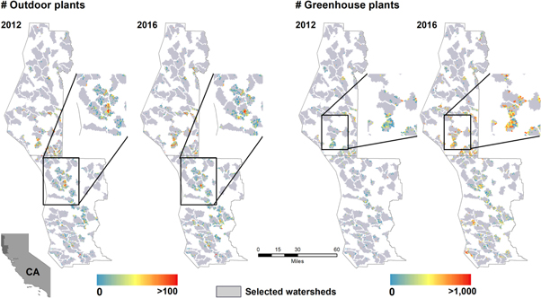
Figure 1. Study area map, outdoor and green house production in 2012 and 2016. Selected watersheds are the ones included in the study.
Download figure:
Standard image High-resolution imageFor greenhouses, it was impossible to confirm that cannabis was being grown inside using aerial imagery. Greenhouses in Humboldt and Mendocino Counties are also used for commercial gardening and nursery operations. To test the plausibility that greenhouses in our study contained cannabis rather than other crops, we tracked greenhouses back to 2004 using National Agriculture Imagery Program (NAIP) imagery for Humboldt County. (This imagery was fine-grained enough to identify greenhouses, but not individual plants in outdoor sites.) Then we compared the growth of greenhouses from 2004–2012 to the growth of the nursery industry during the same period (Humboldt County 2015). From 2004–2012, the abundance of greenhouses increased by 1900%, while the value of nursery products produced in the county fell by 1.5%. This suggests that growth in greenhouses was not likely associated with non-cannabis crops often grown in greenhouses. In addition, the location and size of identified greenhouses—far from markets, main roads, on areas of steep slopes, and less than one acre in size—suggest that they would be unprofitable for crops with market values lower than cannabis. Therefore, we believe that the greenhouses we identified were unlikely to be used for anything but cannabis and we assumed that cannabis is present in each greenhouse we mapped. This may lead to a slight overestimation in cannabis sites if some greenhouses were not used for cannabis.
Overall, we believe the digitizing methodology we employed is robust enough to provide valuable information. There are a few caveats, however, that should be made clear. First, given the nature of the subject, and the fact that digitizing took place years after some of our images were captured, we were not able to ground truth our data. While in the vast majority of the images it is abundantly clear what we are viewing, we were unable to verify cultivation sites on the ground. Second, delineating the boundary of outdoor gardens can be subjective, since there is typically no hard edge to cultivation sites. However, by also counting the number of plants in cultivation sites, we were able to measure the size of sites in both area and potential production.
Describing the expansion of the cannabis frontier
We described the expansion of the cannabis frontier using four different metrics: site count, site size, plant count, and farm count. We defined a cultivation site as any outdoor garden or greenhouse that produces cannabis and we represented each as a polygon in our maps. Farms can, and often do, include multiple cultivation sites. To apply individual-level site statistics to the farm level, we summarized site count, site size and plant count within ownership boundaries, which were provided by Humboldt and Mendocino Counties.
These measures provided unique but complementary information that we used to produce a nuanced and comprehensive description of the expanding cannabis frontier. For example, counting the number of plants was the best way to summarize production, while site size was more useful for describing overall disturbance or land cover change. Similarly, counting individual cultivation sites provided a good description of agricultural expansion (i.e. extensification), while farm or parcel-level summaries provided better information about activities (i.e. intensification) among farmers.
Cannabis expansion and the environment
Direct field measurements of environmental disturbance by cannabis cultivation can be dangerous or impossible to obtain, and depending on how data are collected (i.e. whether or not the product is handled), this work may be federally illegal. Therefore, to understand how the frontier was associated with environmental impact, we combined our maps of cannabis expansion with spatial data on environmental sensitivity. We analyzed four environmental sensitivity proxy variables in relationship to each cultivation site: distance to potential high-quality habitat for coho salmon (Oncorhynchus kisutch), Chinook salmon (Oncorhynchus tshawytscha), and steelhead trout (Oncorhynchus mykiss); distance to paved roads (as a proxy for remoteness); distance to protected public lands; and slope (as a proxy for erosion potential). For each of these indicators we calculated the total and percent increase in site count, site size, and plant count between 2012–2016. We included several ancillary spatial data in our analysis within a Geographic Information System: a digital elevation model (USGS 2013) allowed us to calculate slope, and the National Marine Fisheries Service (NMFS) Intrinsic Potential (IP) habitat datasets for coho and Chinook salmon and steelhead trout habitat allowed us to identify habitat (NMFS 2017) for these US Endangered Species Act-listed species. We identified high-quality habitats as areas with IP values greater than or equal to 0.7 (NMFS 2016). Roads data (US Census 2015) allowed us to calculate remoteness. The California protected area database (http://www.calands.org/data) allowed us to calculate distance from protected public lands.
We chose to focus on these variables for several reasons. For example, salmonids are sensitive to water withdrawals and cannabis production may deplete instream flows (Bauer et al 2015). We examined remoteness because past studies have shown that cannabis farms can contribute to forest fragmentation when located far from roads (Wang et al 2017). Forest fragmentation is generally considered a driver of ecosystem change (Haddad et al 2015). We analyzed slope because soils on steep slopes are prone to erosion when cleared or cultivated (Lal 1990). Furthermore, past land use practices (primarily timber harvest and associated road building) have led to degraded stream quality in our study area due to soil erosion and sedimentation (Madej and Ozaki 1996). Finally, though it is an indirect measure of environmental sensitivity, proximity to protected areas is an indicator of threats posed to conservation values as defined by current environmental policy.
Modeling farm abandonment between 2012–2016
Between 2012–2016 we discovered that 641 farms had stopped producing cannabis. To systematically examine whether farms in more environmentally sensitive areas were abandoned more often than those in less sensitive locations, we used a logit model (Wooldridge 2011) and regressed whether or not a parcel ceased operation (0 = no, 1 = yes) on the environmental variables described above. Because farm abandonment is also likely correlated with the economic condition of the farm, we also include variables that we think may impact farm profitability. First, we include the size of the farm, measured in number of plants as well as acreage. We suspected that larger farms can harness economies of scale and would be more profitable and therefore less likely to abandon. Although many farms import soil and water, we also suspected that farms on prime agricultural lands and those with easy access to water would be less likely to cease operations. Therefore, we also included whether or not a farm was on prime agricultural lands, and the distance from each farm to a stream where they could divert water. Prime agricultural lands for Mendocino County were identified by the State of California Farmland Mapping and Monitoring project (http://www.conservation.ca.gov/dlrp/fmmp). This program does not include Humboldt County, therefore prime agricultural lands in Humboldt were identified via a layer produced by the County itself (https://humboldtgov.org/201/Maps-GIS-Data).
Our objective was to understand better the impetus for cannabis farm abandonment and examine any systematic relationship between abandonment and environmental factors. Logit models are commonly used to understand the associations between variables of interest when the dependent variable is binary and are standard in modeling land use change (Smirnov 2010, Syphard et al 2012). In our case, the regression model took the form:
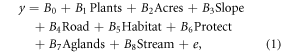
where y is the latent variable (was a farm abandoned), Plants is equal to the estimated number of plants in a site, Acres is equal to the size of the parcel the site is located on, Slope is equal to the average slope of the parcel, Road is equal to the distance to road from the parcel, Habitat is equal to the distance to a stream with threatened or endangered salmon, Protect is equal to the distance to protected area, Aglands is whether a parcel is in prime agricultural lands, Stream is distance to the nearest stream, and e is an error distributed by the logistic distribution.
Regression coefficients from logit models are not easily interpreted, as they are reported in log-odds units. Therefore, using the model results, we predicted the probability of abandonment for each of the variables in the model, across a range of values using the delta method (Oehlert 1992, Williams 2012). By doing this, we can show how changes in each independent variable are associated with changes in the likelihood a site is abandoned, while holding all the other variables constant (figure 3). If farmers' siting decisions are responding to environmental enforcement actions, we would expect that sites with high values for environmental sensitivity would be more likely to be abandoned.
State of California budget allocations to cannabis
Financial allocations to the regulation of the cannabis industry in California during the study period were extracted from each fiscal year's adopted budget bill (State of California 2012, 2013, 2014, 2015b, 2016). Each budget bill was searched for the terms 'cannabis' and 'marijuana', and all resulting allocations were recorded, sorted, and summarized by agency. We chose to focus on budget items that were directly related to environmental protection, and therefore did not include budget items related to general law enforcement, including allocations to the State of California's Campaign Against Marijuana Production, which are not separable from other law enforcement activities in available budget documents.
Limitation of analysis
As with any analysis ours is not without limitations. First, while we believe our method of detecting cannabis cultivation sites is the most accurate currently available, there was undoubtedly some measurement error (e.g. omission and/or commission of polygons). Also, our remote sensing methods cannot identify outdoor cultivation sites under closed forest canopy (though these are likely less productive). When estimating greenhouse production, we made assumptions about plant density and other production practices within greenhouses. For example, we assumed only one crop is grown per year in greenhouses; and, while there is no scientific literature yet on greenhouse production methods, personal communications with many involved in the industry lead us to believe that many farms with greenhouses are producing multiple crops per year. Given this assumption, we believe our estimate of number of plants is quite conservative.
Results
Expanding cannabis production between 2012–2016
Cannabis farms in our study were primarily developed on areas that previously had not been used for agriculture. When checked against the 2006 NLCD (Fry et al 2011) 1% of cultivation sites were developed on pasturelands and 1% were developed on previously-cultivated croplands. 10% of cultivation sites were on developed lands. 88% of sites were developed in areas of natural vegetation, with forest the most common previous land cover, with 41% of the cultivation sites developed on lands that were classified as forest in the 2006 National Land Cover Database. 27% of cultivation sites were developed on shrublands, and the remaining 20% of sites were developed on grasslands.
From 2012–2016 our study area experienced an 80% increase in number of cultivation sites (7847–14 163), a 183% increase in number of plants produced (534 832–1515 425), and a 91% increase in total cultivated area (2.0–3.94 sqkm) (table 1). The overall increase in plants resulted from an increase in sites (extensification) as well as an increase in the number of plants per site (intensification). The increase in plants per site primarily resulted from the increased use of greenhouses. The number of plants grown in greenhouses expanded by 248% between 2012–2016. We saw similar increases in production across all metrics in both Humboldt and Mendocino Counties (table 1). At the individual farm-level we observed similar dynamics. The total number of farms producing cannabis increased by 58% (3749–5906) while on average production per farm increased by 76% (150–264 plants). At the farm level as well, rates of change were similar between counties (figure 2). The average area under cultivation per farm increased from 549 m2 in 2012 to 668 m2 in 2016.
Table 1. Number and changes in cultivation sites, number of plants, and area of cultivation across counties and years.
| Year | County | Number of cultivation sites | Percent increase in number of cultivation sites | Mean number of plants per site | Percent increase in mean number of plants per site | Total plants | Percent increase in total plants | Greenhouse area (km2) | Outdoor area (km2) | Total area (km2) | Percent increase in total area | Average cultivation area per farm (m2) |
|---|---|---|---|---|---|---|---|---|---|---|---|---|
| 2012 | Humboldt | 3783 | 84.82 | 320905 | 0.21 | 0.79 | 1.00 | 654 | ||||
| 2016 | Humboldt | 6656 | 75% | 119.44 | 40% | 795 057 | 147% | 0.6 | 1.09 | 1.70 | 69% | 721 |
| 2012 | Mendocino | 4064 | 53.46 | 217 270 | 0.11 | 0.93 | 1.05 | 476 | ||||
| 2016 | Mendocino | 7507 | 84% | 95.75 | 79% | 718 842 | 230% | 0.54 | 1.70 | 2.24 | 112% | 633 |
| 2012 | Total | 7847 | 68.15 | 534 832 | 0.33 | 1.72 | 2.05 | 549 | ||||
| 2016 | Total | 14 163 | 80% | 106.99 | 56% | 1515 425 | 183% | 1.15 | 2.79 | 3.94 | 91% | 668 |

Figure 2. Identification of cannabis cultivation sites and greenhouses. (A) Typical outdoor cannabis cultivation site as seen using high resolution image from August 2012. Note the distinctive round shape of the plants distinguishes them from other agricultural row crops (such as berries or grapes). The distinctive regular rows and removal of grasses distinguish these plants from natural vegetation. The boundaries of cultivation sites are digitized and polygons are created representing the area of the site (white line). The number of plants in each site are counted and recorded. (B) A clearing in the forest that had potential cannabis plants in August 2012. The size and shape of plants is characteristic of cannabis, but the planting is not in rows and the plants may be native vegetation. Likewise, it is not clear if these plants are recently planted and therefore may be perennial tree crops or natural vegetation. (C) Is an image of the same area from May 2014. In this image we note that the vegetation is not present. Therefore, we conclude that the image from 2012 contains annual plants, and therefore is cannabis. This outdoor cannabis cultivation site would then be digitized in the same manner as that in image (A). (D) Is an image of two greenhouses in 2012. The greenhouses are located on the right side of the picture. On the left side is a metal roofed structure. The perimeters of the greenhouses are digitized. The area of each greenhouse is then calculated, and a number of estimated plants is assigned as 1.115 plants per sq meter, per Bauer et al (2015).
Download figure:
Standard image High-resolution imageRelationship between frontier expansion and environmental indicators
The rapid recent expansion of the cannabis frontier has taken place to a significant degree in ecologically sensitive areas (table 2). By 2016, 20% of all cultivation sites in both counties were located on the 12% of land that exists within 500 m of public protected areas. There was a 102% increase (1376–2780) in number of cultivation sites in these zones. Development also occurred in close proximity to endangered and threatened species habitat, with a 116% increase in number of cultivation sites within 500 m of coho salmon streams, a 97% increase near habitat for Chinook salmon, and an 80% increase near steelhead trout habitat. Cultivation sites continued to be established on steep slopes, with a 76% increase in number of sites (3784–6649) on slopes between 15° and 30° and a 41% increase in sites on slopes greater than 30° (83–117). Finally, cultivation sites continued to be established in remote natural areas, with a 44% increase in new sites more than 1km away from paved roads.
Table 2. Number of cultivation sites in 2012 and 2016 at specific distances from coho salmon, Chinook salmon, and steelhead trout habitat, and paved roads and public lands.
| Coho Salmon | |||||
|---|---|---|---|---|---|
| Distance to habitat | Number of cultivation sites in 2012 | Number of cultivation sites in 2016 | Percent increase in cultivation sites | Percent of total cultivation sites in 2012 | Percent of total cultivation sites in 2016 |
| 0–500 m | 1171 | 2533 | 116% | 14.92% | 17.88% |
| 500 m–1 km | 905 | 1889 | 108% | 11.53% | 13.34% |
| >1 km | 5771 | 9741 | 68% | 73.54% | 68.78% |
| Chinook Salmon | |||||
| 0–500 m | 961 | 1896 | 97.29% | 12.25% | 13.39% |
| 500 m–1 km | 880 | 1651 | 87.61% | 11.21% | 11.66% |
| >1 km | 6006 | 10 616 | 76.76% | 76.54% | 74.96% |
| Steelhead Trout | |||||
| 0–500 m | 2455 | 4412 | 79.71% | 31.29% | 31.15% |
| 500 m–1 km | 2376 | 4102 | 72.64% | 30.28% | 28.96% |
| >1 km | 3016 | 5649 | 87.30% | 38.44% | 39.89% |
| Distance to road | |||||
| 0–500 m | 5869 | 11 129 | 89.62% | 74.79% | 78.58% |
| 500 m–1 km | 963 | 1568 | 62.82% | 12.27% | 11.07% |
| >1 km | 1015 | 1466 | 44.43% | 12.93% | 10.35% |
| Distance to protected areas | |||||
| On public land | 61 | 121 | 98.36% | 0.78% | 0.85% |
| 0–500 m | 1376 | 2780 | 102.03% | 17.54% | 19.63% |
| 500–1000 m | 1103 | 1911 | 73.25% | 14.06% | 13.49% |
| greater than 1 km | 5307 | 9351 | 76.20% | 67.63% | 66.02% |
| Slope | |||||
| 0–5° | 1761 | 4135 | 134.81% | 22.44% | 29.20% |
| 5–15° | 2219 | 3262 | 47.00% | 28.28% | 23.03% |
| 15–30° | 3784 | 6649 | 75.71% | 48.22% | 46.95% |
| greater than 30 | 83 | 117 | 40.96% | 1.06% | 0.83% |
Relationship between cultivation site abandonment and environmental sensitivity
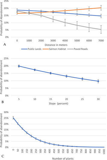
Our regression analysis revealed that the expansion of the cannabis agriculture frontier continued in areas of environmental sensitivity (table 3, figures 3(A) and (B)). The four indicators of environmental sensitivity were all statistically significant when regressed on farm abandonment, but for three of them we found that abandonment was in fact less likely on lands characterized as environmentally sensitive (table 3). Farms close to protected areas were more likely to be abandoned than those far away, indicating that enforcement may have moved farms farther from protected areas. Farms near paved roads were more likely to be abandoned than those located far from paved roads. Likewise, farms close to streams were less likely to be abandoned than those far from steams. Farms on prime agricultural lands were no more likely to be abandoned than farms on non-agricultural lands. The number of plants per farm was a very strong indicator of whether production would cease over the 2012–2016 period (figure 3(B)). Small farms were much more likely to be abandoned than large farms. For example, a farm with 50 plants was twice as likely to cease production as a farm with 200 plants (figure 3(B)).
Table 3. Logit Regression Results. Standard errors in parenthesis. Model one includes all farms. Model 2 includes only farms with at least 25 plants in 2012. Pseudo R2 is 0.089 for model one and 0.93 for model two.
| (1) | (2) | |
|---|---|---|
| Variables | All obs | Larger farms |
| Number of plants | −0.00592c | −0.00576c |
| (0.000 636) | (0.000 706) | |
| Acres of farm | −0.00301b | −0.00351b |
| (0.001 40) | (0.001 66) | |
| Slope | −0.0349c | −0.0408c |
| (0.006 39) | (0.007 91) | |
| Distance to roads | −0.000239b | −6.23e-05 |
| (9.75e-05) | (0.000 103) | |
| Distance to salmon habitat | 4.68e-05b | −6.59e-06 |
| (2.12e-05) | (3.05e-05) | |
| Distance to public land | −5.24e-05b | −9.35e-05c |
| (2.50e-05) | (3.23e-05) | |
| Distance to streams | 0.000562b | 0.000 406 |
| (0.000 227) | (0.000 283) | |
| Prime agricultural lands | −0.0233 | −0.493a |
| (0.189) | (0.273) | |
| Constant | −0.625c | −0.426b |
| (0.126) | (0.167) | |
| Observations | 3749 | 2761 |
Figure 3. Predicted probability for abandonment of cultivation sites as predicted from the logit model including cultivation sites of all sizes. The probability of abandonment refers to the predicted probability that a farm will be abandoned for the value of the variable of interest, holding all other values in the regression at their mean. For example, figure A shows that the probability of a farm being abandoned is roughly 17%, if the farm is very close to a road. However, the farther a farm is from a road, the less likely it is to be abandoned. When a farm is 5 km from a road, there is only a 7% chance it will be abandoned. (A) Probability of abandonment for distance from public lands, habitat and paved roads. (B) Probability of abandonment based on number of plants per farm. (C) Probability of abandonment based on slope.
Download figure:
Standard image High-resolution image
State of California budget allocations to cannabis
During the study period, resources allocated by the State of California to regulating cannabis increased dramatically (table 4). Prior to fiscal year 2014–2015, less than $500 000 per year was allocated for cannabis, and only to the Department of Public Health for administration of a program to identify qualified medical patients. Until 2014–2015, no state funds were allocated for the regulation of cultivation and production. For the first time, starting in 2014–2015, modest allocations were made to state agencies tasked with protecting the environment (table 4).
Table 4. State of California budget allocations to cannabis by fiscal year, by agency.
| Cannabis allocations by fiscal year (US dollars) | ||||||
|---|---|---|---|---|---|---|
| 2011–2012 | 2012–2013 | 2013–2014 | 2014–2015 | 2015–2016 | 2016–2017 | |
| Dept. of Public Health | 461 000 | 482 000 | 208 000 | 138 000 | 574 000 | 3639 000 |
| Dept. of Fish and Wildlife | 500 000 | 503 000 | 7655 000 | |||
| State Water Resources Control Board | 1800 000 | 5685 000 | ||||
| Dept. of Pesticide Regulation | 700 000 | |||||
| California Dept. of Food and Agriculture | 5355 000 | |||||
| Dept. of Consumer Affairs, Bureau of Medical Marijuana Regulation | 1600 000 | 3781 000 | ||||
| Total by fiscal year | 461 000 | 482 000 | 208 000 | 2438 000 | 2677 000 | 26 815 000 |
Allocations increased overall about six-fold by fiscal year 2015–2016, when cannabis growers would have planted their 2016 crops. But 2015–2016 expenditures remained modest in relation to other regulatory priorities. For example, the $2.7 million spent to regulate the cannabis industry in that year was about 7% of what was spent to regulate the timber industry (State of California 2015b), even though cannabis production in the Emerald Triangle alone is worth at least $5 billion annually (ERA Economics 2017) and timber production was only $1.5 billion for the whole state (Mciver et al 2012). Further, only about one-fifth of that funding went towards regulation of environmental impacts associated with cultivation and production (table 4). Following the passage of the Medical Cannabis Regulation and Safety Act (State of California 2015c) in fiscal year 2016–2017, overall allocations increased 58 fold over 2011–2012 numbers to almost $27 million.
Discussion
Agricultural frontiers are hotspots of environmental degradation worldwide, and in this study we document the potential for cannabis, a globally important crop, to create environmentally damaging frontiers. In just five years, we observed a near doubling in the number of cultivation sites and area under cultivation, and a near quadrupling in the number of plants produced. And this rapid expansion took place largely in areas of environmental sensitivity: on steep slopes where erosion poses a threat to water quality and habitat in nearby waterbodies; near streams and rivers harboring endangered species where diversion of surface or groundwater, or pollution from agricultural chemicals, may negatively impact habitat availability; and in remote areas where natural vegetation and habitat is removed to start farms. For example, we found that nearly 90% of the areas developed for cannabis cultivation were formerly covered in natural vegetation as late as 2006. While all of these measures are indirect in the sense that they do not measure specific on-the-ground environmental impacts at individual farms, that kind of comprehensive, site-level data is not available in our study area beyond a handful of cultivation sites where law enforcement activities have taken place. In order to characterize potential for impacts at the watershed or County scale, the use of metrics based on remotely sensed data is necessary.
In our case, this rapid development takes place in California, a state with generally robust environmental laws. However, those laws have not been applied in the cannabis farming context until very recently. Though legalized at the state level for medical production in 1996, the medical cannabis market in California was virtually unregulated in any fashion until 2016 (Stoa 2017), with no state-wide systematic collection of information on cultivation locations or practices. Additionally, there was significant mixing between the state-legal medical market and the illegal market for export within and out of state during this time (Short-Gianotti et al 2017). For these reasons, it is hard to know whether the expansion and land use change we observed took place on farms which were growing for the state-legal, medical market, or for illegal distribution within or outside of California, or for both.
In any case, our analysis supports the hypothesis that one major underlying driver of cannabis cultivation in environmentally sensitive areas has been the paucity of cannabis-specific regulation and enforcement (Carah et al 2015, Short-Gianotti et al 2017). Until 2014–2015, 18 years into state-legal medical cannabis production in California, no state funds had been allocated for the regulation of cultivation and production of cannabis, and only then were modest allocations made to state agencies tasked with protecting the environment. Thus, we interpret the emergence of the cannabis agricultural frontier in northern California during the study period in a context in which there was nearly no investment in cannabis-specific environmental protections, and limited enforcement of existing environmental and land use laws.
Agricultural frontiers are known to challenge institutional development, regulation, and enforcement, and the result is often widespread environmental damage in frontier regions (Lambin et al 2001, Rindfuss et al 2007, Nolte et al 2017). Our results highlight an additional important reality in environmental governance—that a pre-existing framework for regulation is no guarantee of environmental protection in the face of emerging agricultural frontiers. While we do not assume that frontiers are necessarily established everywhere cannabis is grown, we also believe the case of Northern California is not unique: the ability of cannabis cultivation to produce abnormal rent on small pieces of land means that frontiers may emerge almost anywhere institutions fail to prevent it. Given the globally interconnected nature of drug supply and demand, we might expect frontier-like land use activity not only in countries considering future liberalization laws, but also in the 135 countries currently known to produce cannabis for legal or illegal markets, where prohibition may currently drive abnormal economic rents (United Nations Office on Drugs and Crime (UNODC) 2017). Our results should therefore raise attention in other locations where cannabis production may boom in the near term, as they point to an urgent need for the development and enforcement of agricultural and environmental policy specifically designed to address this special crop.
The quasi-legal status of cannabis in many US states has also complicated, and even undermined, regulation of the industry (Stone 2014, Short-Gianotti et al 2017). For example, past attempts by California public agencies to regulate cannabis cultivation have been curtailed by federal authorities (Polson 2017, Short-Gianotti et al 2017). Conflicts like these between state and federal authorities have also incentivized secrecy in production, driving cultivation into clandestine spaces in remote natural areas of high conservation value (Carah et al 2015, Short-Gianotti et al 2017). Federal policy has shifted to some degree in recent years (Ogden 2009, Cole 2013), but federal interventions still limited local regulatory efforts during this period (Butsic and Brenner 2016, Short-Gianotti et al 2017).
While state-level cannabis liberalization with effective regulation may promise to temper the drivers of frontier development, continued federal prohibition simultaneously deepens incentives for frontier development and black market production. Through liberalization one can imagine a path where cannabis production is normalized. Farmers maximize profit by using land that is best suited for growing cannabis instead of areas chosen to avoid detection. Regulators interact with a known clientele to implement environmental protections. Academic and industry research seeks ways to make production as efficient and sustainable as possible. While such a vision may hold the best promise for the environment, as we document here in the first 20 years of cannabis liberalization in California such normalization has been elusive. Whether countries around the globe can actualize such a vision or whether they, too, become home to new environmentally damaging frontiers will likely be driven by the success or failure of cannabis-specific regulatory efforts, as well as consistency or lack thereof in policy at the country and local level.
Acknowledgments
We thank The Nature Conservancy for funding for this project. We also thank over 20 undergraduate students who helped digitize the cannabis cultivation sites. And we would like to thank Michael Polson and Jeanette Howard and two anonymous reviewers who provided thoughtful feedback and suggestions which have improved this manuscript.