James D. Hamilton
Dept. of Economics, University of California at San Diego
Declarations by the Business Cycle Dating Committee of the National Bureau of Economic Research (NBER) are regarded as highly authoritative by academic researchers, policy makers, and the public at large. The NBER’s dates as to when U.S. recessions began and ended are based on the subjective judgment of the committee members, which raises two potential concerns. First, the announcements often come long after the event. For example, NBER waited until July 17, 2003 to announce that the 2001 recession ended in November, 2001. Second, outsiders might wonder (perhaps without justification) whether the dates of announcements are entirely independent of political considerations. For example, there might be some benefit to the presidential incumbent of delaying a declaration that a recession had started or accelerating a declaration that a recession had ended. For these reasons, it is worth exploring whether one could perform a similar function using purely objective summaries of the data.
Any such effort faces a tradeoff between two objectives. On the one hand, we might hope to use as much information in as much detail as possible. On the other hand, the more simple and parsimonious the approach, the more likely it is to prove to be robust as the economy changes and data get revised. The approach described here is based on the second philosophy.
What sort of GDP growth do we typically see during a recession? It is easy enough to answer this question just by selecting those postwar quarters that the NBER has determined were characterized by economic recession and summarizing the probability distribution of those quarters. A plot of this density, estimated using nonparametric kernel methods, is provided in the following figure; (figures here are similar to those in a paper written in 2005 with UC Riverside Professor Marcelle Chauvet, which was published in Nonlinear Time Series Analysis of Business Cycles). The horizontal axis on this figure corresponds to a possible rate of GDP growth (quoted at an annual rate) for a given quarter, while the height of the curve on the vertical axis corresponds to the probability of observing GDP growth of that magnitude when the economy is in a recession. You can see from the graph that the quarters in which the NBER says that the U.S. was in a recession are often, though far from always, characterized by negative real GDP growth. Of the 45 quarters up to the date that paper was written for which the NBER said the U.S. was in recession, 19 were actually characterized by at least some growth of real GDP.
 |
One can also calculate, as in the blue curve below, the corresponding characterization of expansion quarters. Again, these usually show positive GDP growth, though 10 of the postwar quarters that are characterized by NBER as part of an expansion exhibited negative real GDP growth.
 |
The observed data on GDP growth can be thought of as a mixture of these two distributions. Historically, about 20% of the postwar U.S. quarters are characterized as recession and 80% as expansion. If one multiplies the recession density in the first figure by 0.2, one arrives at the red curve in the figure below. Multiplying the expansion density (second figure above) by 0.8, one arrives at the blue curve in the figure below. If the two products (red and blue curves) are added together, the result is the overall density for GDP growth coming from the combined contribution of expansion and recession observations. This mixture is represented by the yellow curve in the figure below.
 |
It is clear that if in a particular quarter one observes a very low value of GDP growth such as -6%, that suggests very strongly that the economy was in recession that quarter, because for such a value of GDP growth, the recession distribution (red curve) is the most important part of the mixture distribution (yellow curve). Likewise, a very high value such as +6% almost surely came from the contribution of expansions to the distribution. Intuitively, one would think that the ratio of the height of the recession contribution (the red curve) to the height of the mixture distribution (the yellow curve) corresponds to the probability that a quarter with that value of GDP growth would have been characterized by the NBER as being in a recession. Actually, this is not just intuitively sensible, it in fact turns out to be an exact application of Bayes’ Law. The height of the red curve measures the joint probability of observing GDP growth of a certain magnitude and the occurrence of a recession, whereas the height of the yellow curve measures the unconditional probability of observing the indicated level of GDP growth. The ratio between the two is therefore the conditional probability of a recession given an observed value of GDP growth. This ratio is plotted as the red curve in the figure below.
 |
Such an inference strategy seems quite reasonable and robust, but unfortunately it is not particularly useful– for most of the values one would be interested in, the implication from Bayes’ Law is that it’s hard to say from just one quarter’s value for GDP growth what is going on. However, there is a second feature of recessions that is extremely useful to exploit– if the economy was in an expansion last quarter, there is a 95% chance it will continue to be in expansion this quarter, whereas if it was in a recession last quarter, there is a 75% chance the recession will persist this quarter. Thus suppose for example that we had observed -10% GDP growth last quarter, which would have convinced us that the economy was almost surely in a recession last quarter. Before we saw this quarter’s GDP number, we would have thought in that case that there’s a 0.75 probability of the recession continuing into the current quarter. In this situation, to use Bayes’ Law to form an inference about the current quarter given both the current and previous quarters’ GDP, we would weight the mixtures not by 0.2 and 0.8 (the unconditional probabilities of this quarter being in recession and expansion, respectively), but rather by magnitudes closer to 0.75 and 0.25 (the probabilities of being in recession this period conditional on being in recession the previous period). The ratio of the height of the resulting new red curve to the resulting new yellow curve could then be used to calculate the conditional probability of a recession in quarter t based on observations of the values of GDP for both quarters t and t – 1. Starting from a position of complete ignorance at the start of the sample, we could apply this method sequentially to each observation to form a guess about whether the economy was in a recession at each date given not just that quarter’s GDP growth, but all the data observed up to that point.
One can also use the same principle, which again is nothing more than Bayes’ Law, working backwards in time– if this quarter we see GDP growth of -6%, that means we’re very likely in a recession this quarter, and given the persistence of recessions, that raises the likelihood that a recession actually began the period before. The farther back one looks in time, the better inference one can arrive at. Seeing this quarter’s GDP numbers helps me make a much better guess about whether the economy might have been in recession the previous quarter. We then work through the data iteratively in both directions– start with a state of complete ignorance about the sample, work through each date to form an inference about the current quarter given all the data up to that date, and then use the final value to work backwards to form an inference about each quarter based on GDP for the entire sample.
All this has been described here as if we took the properties of recessions and expansions as determined by the NBER as given. However, another thing one can do with this approach is to calculate the probability law for observed GDP growth itself, not conditioning at all on the NBER dates. Once we’ve done that calculation, we could infer the parameters such as how long recessions usually last and how severe they are in terms of GDP growth directly from GDP data alone, using the principle of maximum likelihood estimation. It is interesting that when we do this, we arrive at estimates of the parameters that are in fact very similar to the ones obtained using the NBER dates directly, and implied dates for recessions that are very close to those assigned by the NBER.
In that 2005 paper, Chauvet and I explored the potential use of this algorithm as an objective alternative to the declarations of the NBER Business Cycle Dating Committee, taking into account the fact that the data are often revised substantially. For each quarter between 1967:Q1 and 2004:Q2 we assembled from the real-time database at the Federal Reserve Bank of Philadelphia a time series for GDP growth as it would have been reported at that time, fit the parameters of the model to data available at the time, and calculated the implied probability of being in a recession for the next-to-most-recent quarter. The reason for lagging the calculation by one quarter in this way is that data revisions and the extra insight from observing the subsequent quarter’s advance GDP release are necessary in order to form a reliable inference. But if one allows for this extra quarter of smoothing, the inferences seem to be very useful. The following figure plots these real-time probabilities, and is automatically updated using the most recent GDP statistics as described at Econbrowser.
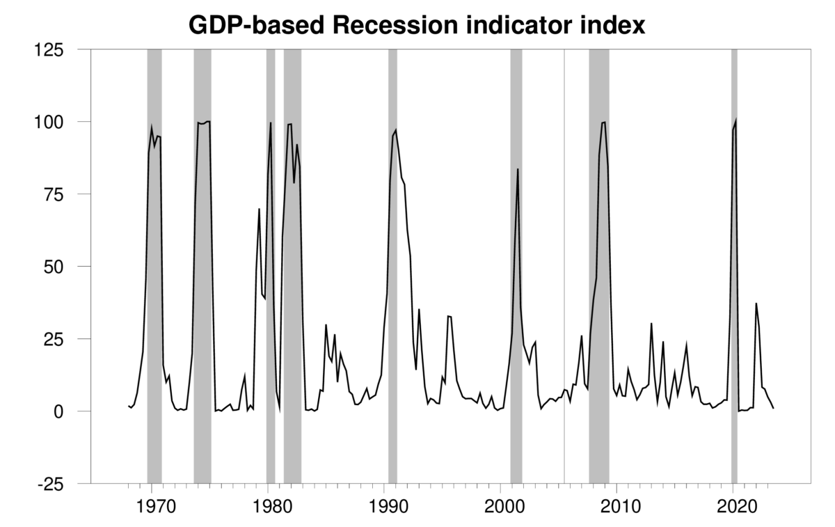
Graph plots for each quarter t the value for Prob(St|Yt+1) where Yt+1 is the history of observed GDP growth rates as reported as of date t+1.
Shaded areas in the above figure denote the dates of NBER recessions, which were not used in any way in constructing the index. Note moreover that this series is entirely real-time in construction– the value for any date is always based solely on information as it was reported in the advance GDP estimates available one quarter after the indicated date, and the series by definition is never revised.
The paper with Chauvet also explored how well an inference based on data as reported in real time would have performed based on the following rule. When the index rises above 67%, we declare the economy to have been in a recession the preceding quarter, and use the full sample of information available as of that point to assign a probable date for the beginning of the recession, defined on the biggest recent value of j for which Prob(St–j=1|Yt) > 1/2 where St=1 indicates a recession. Once a recession has been declared, that announcement remains in effect until the index falls below 33%, at which point an end date for the recession is assigned based on the biggest recent j for which Prob(St–j=1|Yt) < 1/2.
Since July 2005, I have been reporting the value for this index and making these calls on the website Econbrowser each time a new advance GDP figure gets released. A spreadsheet containing these entries can be downloaded here. Note that any individual row of this spreadsheet is by construction never revised, but a new row is added with each new quarter’s data. For rows added since 2005, the last column of the spreadsheet contains hyperlinks to the original release of that row’s numbers with discussion.
Prior to July 2020, we would recalculate the maximum-likelihood estimates of parameters using each new GDP report. The 2020:Q2 observation associated with the COVID recession was such an outlier that it severely distorts maximum-likelihood estimates. One might try to describe the data using three regimes, where the third regime is just the 2020:Q2 observation. What we have done instead (as described
here) is to keep parameter estimates fixed at their values estimated through 2020:Q2 data. Those parameter estimates are mean annualized growth rates for expansion and recession given by 3.87902 and -1.51768, continuation probabilities for expansion and recession given by 0.943698 and 0.696427, and a variance for each regime of 10.1800.
Simulated (prior to 2005) and actual (since 2005) announcements of when recessions began and ended are provided in the following table.
Announcements based on recession indicator index
|
|
|---|---|
| Date of announcement | Announcement |
| Simulated (through June 2005) | |
| May 1970 | recession began 1969:Q2 |
| Aug 1971 | recession ended 1970:Q4 |
| May 1974 | recession began 1973:Q4 |
| Feb 1976 | recession ended 1975:Q1 |
| Nov 1979 | recession began 1979:Q2 |
| May 1981 | recession ended 1980:Q2 |
| Feb 1982 | recession began 1981:Q2 |
| Aug 1983 | recession ended 1982:Q4 |
| Feb 1991 | recession began 1989:Q4 |
| Feb 1993 | recession ended 1991:Q4 |
| Feb 2002 | recession began 2001:Q1 |
| Aug 2002 | recession ended 2001:Q3 |
| Actual real time (since July 2005) | |
| Jan 30, 2009 | recession began 2007:Q4 |
| Apr 30, 2010 | recession ended 2009:Q2 |
| Jul 30, 2020 | recession began 2020:Q1 |
| Jan 28, 2021 | recession ended 2020:Q2 |