Comparison of Methods for Analyzing Left-Censored Occupational Exposure Data

Abstract

The National Institute for Environmental Health Sciences (NIEHS) is conducting an epidemiologic study (GuLF STUDY) to investigate the health of the workers and volunteers who participated from April to December of 2010 in the response and cleanup of the oil release after the Deepwater Horizon explosion in the Gulf of Mexico. The exposure assessment component of the study involves analyzing thousands of personal monitoring measurements that were collected during this effort. A substantial portion of these data has values reported by the analytic laboratories to be below the limits of detection (LOD). A simulation study was conducted to evaluate three established methods for analyzing data with censored observations to estimate the arithmetic mean (AM), geometric mean (GM), geometric standard deviation (GSD), and the 95th percentile (X_0.95) of the exposure distribution: the maximum likelihood (ML) estimation, the β-substitution, and the Kaplan–Meier (K-M) methods. Each method was challenged with computer-generated exposure datasets drawn from lognormal and mixed lognormal distributions with sample sizes (N) varying from 5 to 100, GSDs ranging from 2 to 5, and censoring levels ranging from 10 to 90%, with single and multiple LODs. Using relative bias and relative root mean squared error (rMSE) as the evaluation metrics, the β-substitution method generally performed as well or better than the ML and K-M methods in most simulated lognormal and mixed lognormal distribution conditions. The ML method was suitable for large sample sizes (N ≥ 30) up to 80% censoring for lognormal distributions with small variability (GSD = 2–3). The K-M method generally provided accurate estimates of the AM when the censoring was <50% for lognormal and mixed distributions. The accuracy and precision of all methods decreased under high variability (GSD = 4 and 5) and small to moderate sample sizes (N < 20) but the β-substitution was still the best of the three methods. When using the ML method, practitioners are cautioned to be aware of different ways of estimating the AM as they could lead to biased interpretation. A limitation of the β-substitution method is the absence of a confidence interval for the estimate. More research is needed to develop methods that could improve the estimation accuracy for small sample sizes and high percent censored data and also provide uncertainty intervals.

INTRODUCTION

It is estimated that more than 55000 workers were rostered in the response and cleanup of the oil release from the Deepwater Horizon rig explosion that occurred on April 20, 2010 in the Gulf of Mexico (National Institute for Occupational Safety and Health, 2011). As part of the comprehensive federal response to this effort, the National Institute of Environmental Health Sciences (NIEHS) initiated an epidemiological study (GuLF STUDY) to assess possible adverse health effects associated with exposures from multiple agents to the study subjects who participated in the response and cleanup work.

Exposure assessment is a critical component in the investigation of the exposure-disease relationship and a key criterion used to establish causality (Hill, 1965). During the response and cleanup, personal inhalation exposures were measured by BP, its contractors, and governmental agencies. Over 150000 personal exposure measurements for an array of contaminants were collected; however, a substantial number of these measurements was below the limits of detection (LOD) reported by the analytic laboratories, or left-censored (Type I censoring). These measurements are being used to characterize exposure levels for specific exposure groups defined by factors such as location, vessel, job title/activity, and time period. Despite the large number of measurements, in many cases the number of available measurements for specific exposure groups is small (e.g. <10) and many exposure groups have a high percentage of censored data (50–100% for many groups). In addition, these measurements are often marked by high variability probably due to the non-routine nature of some of the activities and changes in these activities over time. The duration of the samples used in the STUDY varied from 4 to 18h, resulting in multiple LODs. The combination of small sample size, high percentage of censoring, high variability, and multiple LODs presents many challenges to the estimation of the study subjects’ exposures, including the need to identify a methodology for handling such highly censored data sets.

Previous work by Helsel (2005, 2010), European Food Safety Authority (2010), Hewett and Ganser (2007), and Ganser and Hewett (2010) together provide excellent discussions on censored data analysis (CDA) methods typically used in occupational and environmental exposure assessments. Other methods related to epidemiological studies include the multiple imputation approach (Lubin et al., 2004) and a variant of the K-M method, a Cox-regression-based method that was used to assess biomarkers and adverse health effects (Dinse et al., 2014). The general consensus is that all of these methods are better options that the standard substitution method (e.g. LOD/$2$). While some statistical methods for handling left-censored data are available, there is no consensus on the best method for particular situations. For example, Helsel (2005) recommended the Kaplan–Meier (K-M) method, which does not assume any distributional shape of the data, over the maximum likelihood (ML) method for sample sizes of less than 50 and censoring <50%. Hewett and Ganser (2007), on the other hand, recommended the ML method over the K-M method for lognormal and mixed lognormal distributions based on their computer simulations. More recently, Ganser and Hewett (2010) developed the β-substitution method that was either comparable or superior to ML method in most simulated conditions, even for sample sizes of 5–20. However, the K-M method has not been compared with the β-substitution method. No method has been recommended for data with sample sizes of <5 or percent censoring of >80%. While other CDA methods exist, our literature review suggested that the β-substitution, the ML, and the K-M methods were the most promising candidates for further evaluation.

We evaluated these methods for estimating the arithmetic mean (AM), the 95th percentile (X_0.95), the geometric mean (GM), and the geometric standard deviation (GSD). In occupational epidemiology studies, the AM is generally considered the most appropriate metric for calculating cumulative exposure for chronic disease investigation (Seixas et al., 1988; Rappaport, 1991) while the X_0.95 is a useful estimate of the upper bound of a distribution. The three candidate methods were compared in a simulation study to identify the least biased method in the estimation of the AM, X_0.95, GM, and GSD over a wide range of sample sizes (N), variability, and censoring for lognormal and mixed lognormal distributions with a single LOD and with multiple LODs.

BACKGROUND

β-substitution method

This method has its roots in the popular substitution methods where each non-detectable measurement is replaced with LOD/2 or LOD/$2$ (Hornung and Reed, 1990). Unlike the standard substitution methods where 2 or $2$ is arbitrarily chosen, Ganser and Hewett (2010) developed an algorithm that computes a β-factor for adjusting the LOD (i.e. β-factor × LOD). The β-substitution method consists of a series of related intermediate steps that estimate the β-factor to substitute the LOD. The β-factor varies depending on whether the AM or GM is being estimated such that bias is minimized. The AM is computed from the imputed dataset where the LOD is substituted with LOD × β-AM and the GM from dataset where the LOD is substituted with LOD × β-GM. The formulas for estimating the GSD and the 95th percentile are also modified. Interested readers are encouraged to explore the original article by Ganser and Hewett (2010) to see the entire algorithm (the derivation of the β-factor is also provided in the Supplementary data at Annals of Occupational Hygiene online). The β-substitution method assumes a lognormal distribution of the data. The algorithm can be easily implemented in a simple spreadsheet or statistical software.

Maximum likelihood (ML) estimation method

The ML method can be traced back to work by Fisher (1925) and Cohen (1959, 1961). Exposure data are log-transformed where µ = ln(GM) and σ = ln(GSD). The ML estimates are values of µ and σ that maximize the likelihood function.

where n = number of detectable measurements, m = number of non-detectable measurements, x_i values = detectable measurements, LOD_i values = detection limits, PDF = normal probability density function, and CDF = normal cumulative distribution function. Most statistical programs have built-in optimization algorithms to solve this equation. There are several variations of ML methods; however, the difference in the performance of these methods was found to be minor (Hewett and Ganser, 2007). In this article, we used a standard ML method (Cohen, 1950, 1959).

In our review of the occupational hygiene literature concerning CDA, we found two approaches for estimating the AM from lognormal data. One is the maximum likelihood estimator (MLE) (Cohen, 1950, 1959) and the other is the minimum variance unbiased estimator (MVUE) (Finney, 1946; Aitchison and Brown, 1969), which we will now name as ML_MLE-AM and ML_MVUE-AM, respectively. The maximum likelihood estimate of the AM is:

where $μ^$ and $σ^$ are the maximum likelihood estimates of the parameters µ and σ obtained by maximizing the likelihood function for the log-transformed censored data. The maximum likelihood estimates are asymptotically unbiased and efficient, thus the ML method is generally recommended for moderate to large sample sizes (Helsel, 2005; Hewett and Ganser, 2007; Krishnamoorthy et al., 2009)

The MVUE of the AM is:

where

In this expression, $μ^$ and $σ^$ are the sample mean and standard deviation, $g=σ^2/2$, and n = sample size. Calculation of the first five terms of this infinite sum usually provides sufficiently precise estimates (Hewett and Ganser, 1997).

The MVUE of the AM is typically used for noncensored data with small sample sizes. However, Hewett and Ganser (2007) found that ML_MVUE-AM also provided accurate estimates of the AM using ML estimates of µ and σ for censored data in place of the sample mean and standard deviation as it helps to correct the bias that occurs from transforming estimates from the logarithmic scale back to the untransformed scale. These two computations for the AM of the ML method do not apply to the computation of the X_0.95, GM, or GSD.

Reverse Kaplan–Meier method

The K-M method is a non-parametric method that does not assume any underlying probability distribution of the data (Kaplan and Meier, 1958). Originally developed for analyzing right-censored survival data, the reverse algorithm was adapted to handle left-censored data. The K-M algorithm constructs a curve akin to an empirical CDF where it assigns a probability to each of the ranked detectable measurements while adjusting for censoring. If there are no censored values, the K-M curve is equivalent to the empirical CDF. Most statistical software packages (e.g. Minitab, SAS, or R) have procedures to calculate K-M estimators for right-censored survival analysis. Users can use the same procedures for left-censored data by ‘flipping’ the data (turning it from left-censored to right-censored) and then returning it back to the original scale after the probabilities have been computed. For the X_0.95 calculation, we used the algorithm denoted as Q6 in Hewett and Ganser (2007): (i) sort the data from low to high; (ii) calculate i = integer portion of 0.95 (n + 1); (iii) $X^0.95$= x_i + (0.95 (n + 1) − i) (x_i+1 − x_i). The required minimum sample size of computing the X_0.95 is 20. We used the reverse K-M algorithm published in the US EPA ProcUCL 4.0 Software Technical Guide (U.S. Environmental Protection Agency, 2007) and examples by Beal (2010) for our simulation study (the K-M algorithm can be found in the Supplementary data at Annals of Occupational Hygiene online).

METHODS

Simulation design

The accuracy of an estimation method to treat censored data depends on the assumed distributional shape of the data, the sample size, the degree of censoring, and the variability of the data. To assess the effect of each of these conditions, we generated simulated censored data sets from lognormal distributions and from mixed lognormal distributions for varying sample sizes, degrees of censoring, and GSDs with a single and with multiple LODs.

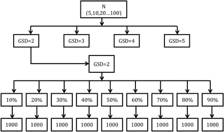
Figure 1 summarizes our simulation design for the three types of simulations that were conducted for this study. In Simulation 1, uncensored values of various sizes were randomly drawn from lognormal distributions with a true GM = 1 and true GSDs = 2, 3, 4, and 5. Sample sizes were 5, 10 and then were incrementally increased in steps of 10 up to 100. The target censoring was first fixed at 10% and was then incrementally increased in steps of 10–90%. We then selected a LOD value from each distribution that corresponded to the expected censoring level. For example, if the percent censoring was p, then LOD = X_p, where X_p is the value at the p percentile. Values that were less than or equal to the LOD were censored to create each final dataset. For each combination of N, GM, GSD, and expected percent censoring, 1000 datasets were generated and the four parameters (AM, GM, GSD, X_0.95) were estimated using the β-substitution, the ML, and the K-M methods.

Simulation 2 was similar to Simulation 1 except that three LODs were generated. LOD₁ was set equal to the value at the percentile p₁ of the distribution that corresponded to the expected level of censoring. LOD₂ was at the percentile that was 5% less than p₁ (i.e. p₁ × 0.95), and LOD₃ was at the percentile 10% less than p₁ (p₁ × 0.90). For each data set, values were randomly assigned to one of the three LODs with equal probability. A value was censored if it was less than or equal to its assigned LOD. The choice of these levels of LODs was based on the rationale that differing LODs in a dataset are typically close to one another due to the small variability in the sampling rates of active sampling methods (rates of passive methods are constant), in sampling times (when attempting to sample full-shift exposures), and in the analytic methods. Because LOD₂ and LOD₃ are simulated to be less than LOD₁, which is at the assigned percent censoring of the distribution, the final percent censoring in the multiple LODs simulation is always slightly less than the expected percent censoring.

In Simulation 3, a mixed lognormal distribution was created by combining two randomly drawn lognormal distributions, each of which contributed 50% to the mixed distribution. The mixed distributions were simulated to represent conditions that comprise two exposure groups with different exposure distributions that cannot be distinguished from each other because of limited descriptive information.

Two types of mixed lognormal distributions were simulated. The first comprised two lognormal distributions with a GM₁ = 1 and a GM₂ = 5 and the second with a GM₁ = 1 and a GM₂ = 10. In both simulations, the GSDs for each contributing lognormal distribution were fixed at 2, 3, 4, and 5. For example, at GSD = 2 the first distribution had a GM₁ = 1 and a GSD₁ = 2 and the second distribution had a GM₂ = 5 and a GSD₂ = 2. Three LODs were generated and values were censored as in Simulation 2. Only the AM and X_0.95 parameters were evaluated for the mixed distribution conditions.

As in all simulations, the observed censoring for a given dataset may deviate from the expected censoring. Datasets that were 100% censored (observed) were discarded because all methods used here are inappropriate for 100% censored data. Hundred percentage of censored datasets occurred more frequently under high censoring and small sample size conditions. At a given expected censoring percentile, p, and a given sample size, N, we expect to observe datasets with 100% censoring with a probability p^N (e.g. when N = 5 and p = 80%, the expected percent of 100% censored datasets = 32.76%).

Simulations were programmed in statistical computing software R (R Development Core Team, 2013).

Evaluation metrics

We compared the methods using relative bias and rMSE found in Hewett and Ganser (2007). Relative bias (called bias hereafter) is the difference between the average of estimated values and the true value relative to the true value.

where θ is the true value of the parameter of interest (i.e. AM, GM, GSD, and X_0.95) and $xˉ$ is the mean of the 1000 corresponding parameter estimates. Bias can be negative or positive. Negative bias means the method underestimated the true value of the parameter while positive bias denotes overestimation of the true value.

The rMSE is a measure that combines the bias and the precision of the method relative to the true value. rMSE can only be positive.

The smaller the bias and rMSE, the better the performance of the method.

RESULTS

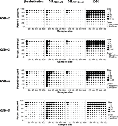
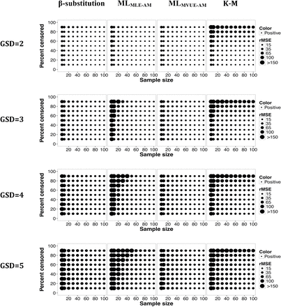
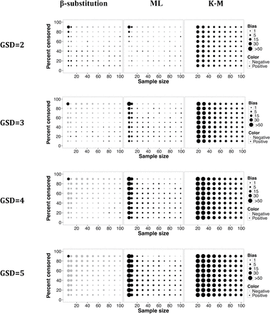
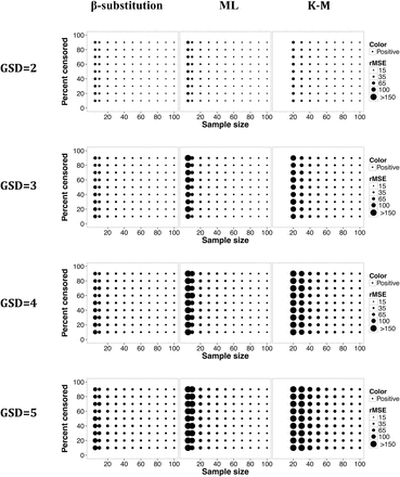
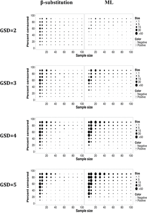
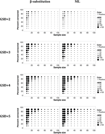
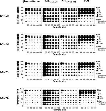
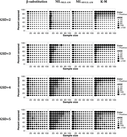
The estimates of bias and rMSE for the AM, X_0.95, GM, and GSD in Simulations 1 and 2 (lognormal distribution with a single LOD and lognormal distribution with multiple LODs) were very similar. Only figures for the AM, X_0.95, and GSD with multiple LODs are shown in this article. Results for the GM from the lognormal distributions with multiple LODs (Simulation 2, Figs 1 and 2), for all the parameters from the lognormal distributions with a single LOD (Simulation 1, Figs 3–10), and for mixed distributions (Simulation 3, Figs 11–16) are provided in the Supplementary data at Annals of Occupational Hygiene online. The bias and rMSE were computed from each set of conditions for each of the four parameters. In the figures, the size of the circle corresponds to the magnitude of the bias or the rMSE on a continuous scale. The legend on the right side of the figures shows circles corresponding to specific values. Thus, the size of each circle in the figures generally falls between two circles in the legend. The largest circle in the legend is interpreted as either equal to or greater than 50% (for bias) or 150% (for rMSE). The figures are intended to provide an overview of the range of conditions evaluated. The actual numbers are included in the Supplementary data at Annals of Occupational Hygiene online (Excel file). In this presentation, we refer to GSDs of 2–3 as low variability and GSDs of 4–5 as high variability. Sample sizes of 5, 10, and ≥20 are considered to be small, moderate and large sample sizes, respectively. Censoring of <50 and ≤80% are described because they appear to be the breakpoints where one or more of the methods’ performances changed. Generally, the bias and rMSE increased (the estimates became less accurate and precise) as the sample size decreased, the percent censoring increased, and/or variability (GSD) was high.

Lognormal distribution for multiple LODs

Arithmetic mean

Figures 2 and 3 present the bias and rMSE results for the AM for a lognormal distribution with multiple LODs. Overall, the β-substitution method generally produced comparable or smaller bias and rMSE compared to the ML and K-M methods, even under small and moderate sample size conditions. When the variability was high, the β-substitution and the ML_MVUE-AM methods produced similar bias and rMSE. Under small N, high variability and high percent censoring conditions, the bias and rMSE for the ML_MLE-AM method were higher compared to the β-substitution and the ML_MVUE-AM methods, indicating that the ML_MLE-AM method was generally less accurate and less precise than the β-substitution and the ML_MVUE-AM methods. The poor performance of the ML_MLE-AM approach was mainly due to bias occurring from deriving the AM from the GM and GSD. The use of the MVUE equation appeared to mitigate this problem in the ML method as evident by the small bias and rMSE of the ML_MVUE-AM method.

The K-M method’s bias, for the most part, was comparable to the β-substitution and ML_MVUE-AM methods when censoring was <50% and sample sizes were moderate to large, regardless of the GSD evaluated. The rMSE of the K-M method generally increased under small to moderate sample conditions and/or high censoring (≥80%), indicating less precision under those conditions.

All three methods generally were observed to have similar rMSEs under the condition of large Ns and censoring level approximately ≤80%. The β-substitution and the ML_MVUE-AM methods tended to underestimate the true AM (negative mean bias), whereas the ML_MLE-AM and K-M methods tended to overestimate the true AM (positive mean bias).

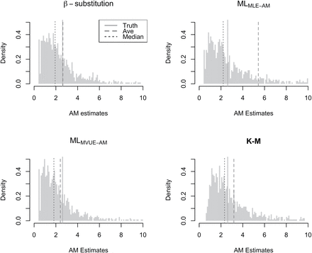
We also found that the distributions of the estimates from the 1000 datasets for small sample sizes conditions were typically skewed. Figure 4 shows an example of the distributions of the AM estimates under the condition of N = 5, GM = 1, GSD = 4, and p = 40%. The ML_MLE-AM equation tended to produce more extreme estimates of AM (longer tail) compared to the other methods, resulting in the average of the AM estimates being much larger than the median and the true AM (although this was less of an issue when Ns were very large). This is an example where the use of bias could be misleading (i.e. the presence of extreme values resulting in a higher average value than the values of a large majority of the estimates). In other instances, a method may yield a low bias even though the bias is a result of averaging very low and very high estimates of the parameter compared to the true value. For such cases, the rMSE is a better metric of the method’s performance.

95th percentile

Figures 5 and 6 show that the bias and rMSE in the estimation of the X_0.95 from the β-substitution method generally were similar or smaller than for the ML and the K-M methods, even for small and moderate samples. The bias and rMSE of the ML and K-M methods were adversely affected by both small sample size and by high levels of censoring. As the variability increased, the bias and rMSE for all three methods increased, particularly for small to moderately sample sizes. The β-substitution was least affected of the three methods. The β-substitution method tended to underestimate the true X_0.95 whereas the ML and the K-M methods generally overestimated the true X_0.95.

GSD

As shown in Figs 7 and 8, the bias and rMSE found for the estimation of the GSD from the β-substitution and the ML methods were comparable in most simulated conditions; however, at high variability under the conditions of small to moderate sample sizes, the ML method’s bias and rMSE were greater than those of the β-substitution method. Both the ML and the β-substitution methods tended to overestimate the GSD and produce extreme values as indicated by the high rMSE. The non-parametric K-M method does not compute the GM and GSD.

Mixed lognormal distribution and multiple LODs

Arithmetic mean

The bias and rMSE of the mixed distributions where the true GMs were 1 and 5 were similar to the results from those of a lognormal distribution (Figs 11 and 12 in the Supplementary data at Annals of Occupational Hygiene online). This is probably due to the modes (GMs) of the two distributions being relatively close to each other so that the resultant distributions more resembled lognormal distributions than the intended mixed distributions.

Figures 9 and 10 show the bias and rMSE from the mixed distribution where the true GMs were 1 and 10. The β-substitution method generally produced comparable or smaller bias and rMSE than the ML and the K-M methods. The β-substitution method, although being a parametric method, appeared to be less sensitive to the mixed distribution than the ML methods. The K-M method had low bias for censoring up to 50% and high rMSE under small sample sizes conditions.

DISCUSSION

Our simulations covered a wider range of N, GSD, and percent censored than previous studies. First, we compared four important parameters: the AM, the X_0.95, the GM and the GSD. We covered sample sizes as low as 5 and GSDs that represented very routine, well controlled situations (GSD = 2) and unusual situations, such as where non-routine work is being carried out (GSD = 5). We evaluated high levels of censoring (up to 90%) that may be applicable to many of today’s workplaces that are very well controlled. We simulated the condition of multiple LODs, which can occur due to varying durations of the measurements and sampling and analytic methods. Finally, we evaluated mixed distributions, which can occur when grouping disparate measurements that have limited sampling documentation. Thus, most of the conditions likely to be encountered by the practitioner have been investigated.

In comparing the ML and the K-M methods, we found inconsistent recommendations in the literature. Hewett and Ganser (2007) recommended the ML method over the K-M method at percent censoring ≤50% even for small N and mixed distributions. Helsel (2005, 2010), on the other hand, preferred the K-M method over the ML method for N ≤ 50 and censoring ≤50%, although the ML method was recommended for N ≥ 50 and censoring 50–80%. His suggestion was based on reviews of published studies (e.g. Shumway, 2002; Antweiler and Taylor, 2008) that mostly evaluated the population mean and other non-lognormal summary statistics, such as the median and standard deviation. These inconsistent recommendations for the mean could be due to the the use of different equations for calculating the AM in the ML method. Our simulation results showed that the K-M method generally had a lower bias and rMSE than the ML_MLE-AM method for censoring ≤50% in the estimation of the AM, particularly for small and moderate sample sizes. However, at censoring >50% and large sample size conditions, the ML_MLE-AM was generally comparable or better than the K-M method. Our results comparing the ML_MLE-AM with the K-M methods were generally in line with Helsel’s recommendation of the K-M method and other studies (Cohn, 1988; Shumway et al., 2002). A comparison of the bias and rMSE of the K-M method with the ML method using the MVUE equation, however, led us to similar conclusions as Hewett and Ganser’s.

We therefore suggest that practitioners apply these recommendations with care, taking into consideration their data, their needs and the uses of the statistical analysis. For example, the Minitab and the NADA packages that were referenced in Helsel’s book (Helsel, 2005) used the ML_MLE-AM equation. If a practitioner follows Hewett and Ganser’s recommendation to use the ML method even for small sample sizes, without knowing which formula the package uses to calculate the mean, a misinterpretation of the results could occur.

Those practitioners who are assessing compliance with occupational exposure limits may be interested in the X_0.95 of the measurements and therefore may not be concerned with the different formulas used to calculate AMs. Occupational exposure assessment strategies focused on compliance often rely on the lognormality assumption to obtain recommended statistics (Ramachandran, 2005; Ignacio and Bullock, 2006), which typically do not include the AM, but include the GM, GSD, and X_0.95. Compliance assessments also typically involve prioritization of exposure groups with only the highest exposure groups being monitored. This prioritization process, therefore, likely results in exposure groups with a lower degree of censoring than what we see in the GuLF STUDY.

Our purpose of assessing occupational exposures for the GuLF STUDY is different from the above. The AM is typically used to compare and contrast exposure groups in an epidemiologic study looking at chronic effects, while the X_0.95 may be used for studying effects of peak exposures. Since all exposure groups must be assessed in an epidemiologic study, it is more likely that there will be exposure groups with highly censored data (>50%). Thus, we needed to identify a method that developed estimates with acceptable bias and error in the presence of high levels of censoring.

As with any computer simulation study, it is worthy to note that for a given dataset (especially a small dataset), the true underlying distribution is often unknown, and the percent censoring from the data does not necessarily correspond to the actual percentile in the true distribution used in our simulations. Hence, the true bias will probably differ from the composite bias obtained from these simulations and thus, the bias reported here cannot be assumed to be the bias of any particular dataset even though it meets the conditions we evaluated. However, these simulations serve as good evaluation tools to compare the methods when subjected to the same conditions. We also used only two distributions to evaluate the effect of mixed distributions, and the resultant distribution more resembled slightly contaminated data rather than an extreme case of mixed distributions. If the modes of the data were clearly not lognormal (GM₁ = 1 and GM₂ = 100) and highly censored, then it is possible that no currently available method is appropriate. The effect of multiple LODs was evaluated by taking two lower percentiles of the highest LOD. Another approach would have been to use LODs sampled from a distribution centered around a single value. We did not take this approach for ease of interpretation of the LOD values. The alternative approach would likely have resulted in similar bias and rMSE if the differences among the LODs were small. Another limitation of our study is that we did not evaluate the uncertainty of the estimates. Estimation of uncertainty was, however, beyond the scope of this work. Also, we simulated conditions that are generally found in typical, routine workplace operations; the operations in the GuLF STUDY were often non-routine, and therefore may not have been covered by our simulation conditions.

CONCLUSIONS

This simulation study was conducted to identify a methodology to handle the highly censored data found in the GuLF STUDY. The β-substitution method performed better than the ML and the K-M methods under most conditions of our study (including low N, high censoring, high variability, multiple LODs, and mixed distributions) using relative bias and relative rMSE as the evaluation metrics. The β-substitution method’s accuracy and precision decreased at small and moderate sample sizes (N ≤ 10), but was still the best of the three methods. Estimates for sample sizes <5 are likely to be unreliable. The ML generally did well with large samples sizes and lognormal distributions. The use of the MVUE equation in the estimation for the AM using the ML method estimates of the GM and the GSD reduced the ML’s transformation bias to the AM for small to moderate sample sizes. The K-M method was generally less biased at censoring levels <50%. Though very robust, a major limitation of the β-substitution method is the lack of a confidence interval around the mean, whereas confidence intervals can be computed for the ML and the K-M methods. This study suggests that none of the statistical methods evaluated in this article are recommended for datasets that have a combination of small to moderate sample sizes, high levels of censoring, or high variability. There is a need for the development of other methods that could improve the accuracy under those conditions and could also provide the uncertainty estimates. A Bayesian approach that allows the use of prior information (e.g. professional judgment, mathematical models) to provide information on the distribution of the dataset may help to improve the estimation in these scenarios.

FUNDING

Intramural Research Program of the NIH, National Institute of Environmental Health Sciences (ZO1 ES 102945).

REFERENCES