

Abstract
Coastal forests sequester and store more carbon than their terrestrial counterparts but are at greater risk of conversion due to sea level rise. Saltwater intrusion from sea level rise converts freshwater-dependent coastal forests to more salt-tolerant marshes, leaving 'ghost forests' of standing dead trees behind. Although recent research has investigated the drivers and rates of coastal forest decline, the associated changes in carbon storage across large extents have not been quantified. We mapped ghost forest spread across coastal North Carolina, USA, using repeat Light Detection and Ranging (LiDAR) surveys, multi-temporal satellite imagery, and field measurements of aboveground biomass to quantify changes in aboveground carbon. Between 2001 and 2014, 15% (167 km2) of unmanaged public land in the region changed from coastal forest to transition-ghost forest characterized by salt-tolerant shrubs and herbaceous plants. Salinity and proximity to the estuarine shoreline were significant drivers of these changes. This conversion resulted in a net aboveground carbon decline of 0.13 ± 0.01 TgC. Because saltwater intrusion precedes inundation and influences vegetation condition in advance of mature tree mortality, we suggest that aboveground carbon declines can be used to detect the leading edge of sea level rise. Aboveground carbon declines along the shoreline were offset by inland aboveground carbon gains associated with natural succession and forestry activities like planting (2.46 ± 0.25 TgC net aboveground carbon across study area). Our study highlights the combined effects of saltwater intrusion and land use on aboveground carbon dynamics of temperate coastal forests in North America. By quantifying the effects of multiple interacting disturbances, our measurement and mapping methods should be applicable to other coastal landscapes experiencing saltwater intrusion. As sea level rise increases the landward extent of inundation and saltwater exposure, investigations at these large scales are requisite for effective resource allocation for climate adaptation. In this changing environment, human intervention, whether through land preservation, restoration, or reforestation, may be necessary to prevent aboveground carbon loss.
Export citation and abstract BibTeX RIS

Original content from this work may be used under the terms of the Creative Commons Attribution 4.0 license. Any further distribution of this work must maintain attribution to the author(s) and the title of the work, journal citation and DOI.
1. Introduction
Coastal forests sequester and store more carbon per unit area than upland forest (McLeod et al 2011; Simard et al 2019), storing carbon both near-term in aboveground biomass and longer-term in sediments (Duarte and Prairie 2005, Poulter et al 2008, Noe et al 2016, Krauss et al 2017). Despite their limited global extent, they play a disproportionately important role in the global carbon cycle (Poulter et al 2006; Henman and Poulter 2008). Through sequestration and storage, coastal forests provide critical ecosystem services that help regulate global climate and mitigate climate change (MEA 2005, McLeod et al 2011). However, these coastal systems are shrinking precipitously due to human land-use modifications and sea level rise (McLeod et al 2011, Pendleton et al 2012). As sea levels rise, inundation, saltwater intrusion, and land loss will increase (Church and White 2011, Church et al 2013, Dangendorf et al 2017), compounding the negative impacts from human pressures (He and Silliman 2019). Coastal systems have always been considered dynamic and resilient (Kirwan and Megonigal 2013), however, their ability to adapt to this rapid change is uncertain.
The freshwater-dependent plant species characteristic of temperate coastal forests have varying tolerances to inundation and salinity. Initially, exposure primarily impacts seedlings by inhibiting regeneration (Brinson et al 1995, Williams et al 1998, DeSantis et al 2007, Krauss et al 2009, Langston et al 2017). Mature trees can generally withstand short periods of inundation and exposure, but prolonged exposure leads to osmotic stress and eventual mortality (Kirwan et al 2007, Conner et al 2007, Krauss et al 2018).
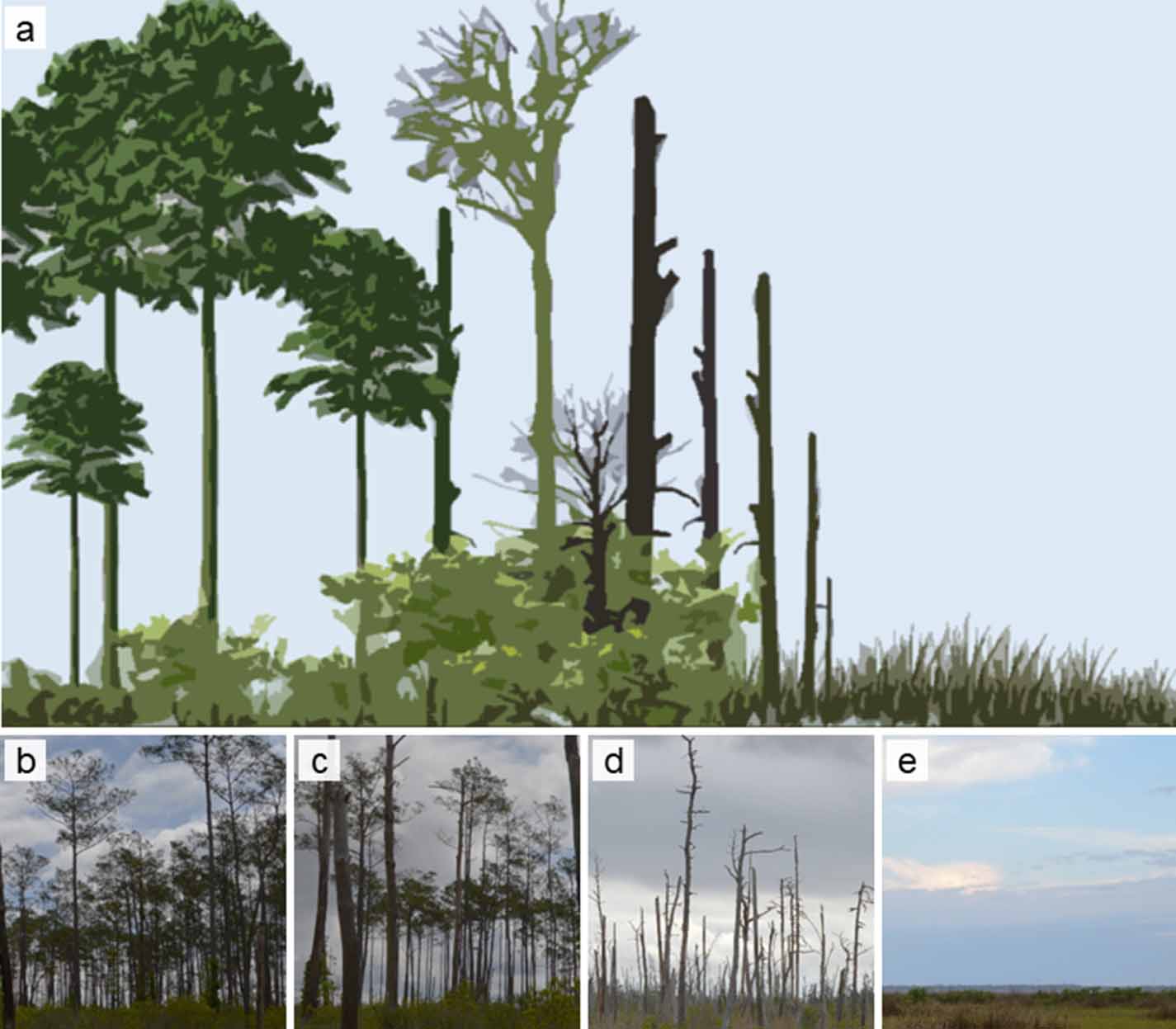
In response to increased salinization and inundation, freshwater-dependent coastal forests are retreating upslope, leaving behind dead trees surrounded by salt-tolerant shrubs and herbaceous plant species (Hackney and Yelverton 1990, Williams et al 1999a). This conversion can occur over the course of a decade or more (Craft 2012, White and Kaplan 2017). These 'ghost forests' are common along the North Atlantic Coast and Gulf of Mexico, varying geographically in extent and conversion rates due to spatial variation in plant community composition (Poulter et al 2008, 2009, Kirwan and Gedan 2019) and relative sea level rise rates (Karegar et al 2016, 2017). Ghost forests are part of a transition zone between coastal forest and marsh (figure 1), and can remain visible on the landscape for decades after the forest has functionally transitioned to marsh (Williams et al 1999b, Moorman et al 1999), serving as late-stage indicators of saltwater intrusion.
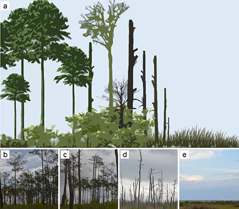
Figure 1. (a) Schematic of the forest-to-marsh transition gradient typical in eastern North Carolina, USA. (b) Coastal forests, dominated by loblolly pine (Pinus taeda), bald cypress (Taxodium distichum), or pond pine (Pinus serotina), give way to (c) 'transition forest' with an abundance of shrub and herbaceous species that have higher salt tolerances. (d) In later stages, marked by a greater number of dead standing trees, transition forest is generally referred to as 'ghost forest.' Without competition from tree seedlings, salt-tolerant marsh species migrate into the area (referred to as marsh migration), completing the transition to (e) herbaceous marsh comprised of brackish or saline herbaceous plant species like sawgrass (Cladium jamaicense) and black needlerush (Juncus romerianus). (Image credit: L S Smart.)
Download figure:
Standard image High-resolution imageMulti-layered and structurally complex coastal forests transition to marshes with very little complexity following saltwater intrusion. Losses in structural complexity have important implications for carbon storage. Because aboveground carbon is closely linked with plant height (Jenkins et al 2003), we expect that conversion from forest to marsh will decrease aboveground carbon storage. As evidenced in other biomes, the transition from forest to herbaceous plant communities (e.g. grasslands) decreases aboveground carbon storage and increases albedo, which exacerbates the effects of greenhouse gases (Gibbon et al 2010, Kirschbaum et al 2012). In coastal systems, the impacts of ghost forest proliferation on ecosystem services, particularly carbon storage, are understudied (Conner et al 2007, Erwin 2009, Tully et al 2019). The broad spatial and temporal extents at which conversion occurs make measurement particularly difficult. Making quantification even more difficult, local-scale factors such as salinity gradients, wind tides, surface water flow, and geologic activity (e.g. subsidence), create fine-scale heterogeneity across these broad extents (Ardón et al 2013, Herbert et al 2015).
We integrated multiple sources of remote sensing data and field data to quantify changes in aboveground carbon storage across a large low-lying coastal region in North Carolina, USA. Past studies examining landscape-scale changes in coastal forests have focused on tropical mangrove forests (e.g. Hamilton and Casey 2016, Thomas et al 2017) not freshwater-dependent temperate forests (however, see Raabe and Stumpf 2016, Schieder et al 2018), and have not addressed associated aboveground carbon storage dynamics (however, in mangrove forests, see Lagomasino et al 2019). To our knowledge, ours is the first study to examine landscape-scale aboveground carbon dynamics related to ghost forest proliferation, a phenomenon unique to temperate regions. Our objectives were to (1) map the 13-year spread of ghost forests in a large low-lying coastal region, (2) quantify the associated loss in aboveground carbon, and (3) compare forest loss from ghost forest spread to other sources of disturbance (e.g. wildfires and forestry activities). Because coastal forests serve as buffers against storm surges (Barbier et al 2011), provide habitat for wildlife species (Field et al 2016, Taillie et al 2019), and preserve productivity of lands in coastal communities (McNulty et al 2015, Tully et al 2019), the ability to identify landscape-scale transitions from forest to marsh is ecologically and economically important. The carbon dynamics related to this unique transition also highlight a potentially important positive feedback loop between climate change and greenhouse gas emissions (Henman and Poulter 2008). By examining spatio-temporal patterns in ghost forest extent and aboveground carbon, we demonstrate how saltwater intrusion from sea level rise impacts important carbon pools in temperate coastal forests. As sea level rise accelerates, landscape-scale measurements of this phenomenon are integral to a better understanding of the impacts of climate on the global carbon cycle and the continued persistence of critical ecosystem services.
2. Methods
Our study area was an approximately 4000-km2 portion of the Albemarle-Pamlico Peninsula in eastern North Carolina, USA, buffered from the Atlantic Ocean by a chain of barrier islands and the Albemarle and Pamlico Sounds. Almost half (47%) of the peninsula is < 1 m in elevation (figure 2(a)); the region is therefore highly vulnerable to sea level rise impacts, and saltwater intrusion has already caused forest decline here (Young 1995, Moorhead and Brinson 1995, Poulter 2005). Forty percent of the lands on the peninsula are publicly owned; most of these are 'unmanaged'. We refer to these areas as 'unmanaged' because there are no extractive activities, but they may be managed for biodiversity, which can include mimicking disturbance events (e.g. controlled or prescribed burning to imitate natural fire disturbances) and controlling water flow. Managed public lands refer to lands that are subject to extractive use (e.g. logging or mining) (figure 2(b)). Privately held lands are comprised of a mix of natural forest, agriculture, and forestry uses (figure 2(b)).
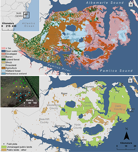
Figure 2. (a) The Albemarle-Pamlico Peninsula in eastern North Carolina, showing landcover (National Land Cover Database 2016 data) and areas less than 1 m in elevation. (b) Unmanaged and other public lands on the Albemarle-Pamlico Peninsula in eastern North Carolina. Ninety-eight field plots were established across five sites in the study area. At each site, plots were established across a vegetation gradient: forest, transition-ghost forest, and marsh (see example in inset map; forest plots are green, transition-ghost forest plots are yellow, and marsh plots are blue).
Download figure:
Standard image High-resolution imageWe collected field data at five sites along the shoreline of the Albemarle-Pamlico Peninsula. Each site was accessible by road, under 1 m in elevation, and publicly owned (no active management at the site). At each site, we sampled evenly across the forest-marsh gradient by delineating three vegetation zones (forest, transition-ghost forest, and marsh) using aerial photographs and confirmed these in the field as part of the sampling protocol (Poulter et al 2005). We randomly selected seven 12-m-radius vegetation plots in each zone (figure 2(b)). At each plot, we recorded species name, diameter at breast height (DBH), and height for live woody species greater than 2.5 cm in diameter; for vegetation less than 1 m in height, we recorded percent cover within five 1-m2 subplots. We averaged percent cover across the five subplots to obtain an average cover value for each species. We calculated the aboveground biomass of each plant documented in the field by applying species-specific allometric equations (table S3; Smith and Brand 1983; Jenkins et al 2003; Castillo et al 2008; Trilla et al 2009; Riegel et al 2013). For each plot, we summed all aboveground biomass values and converted them to a per-unit area estimate (Mg ha−1). Each site had 21 plots, except for one site, which had no marsh zone (14 plots). We first inventoried vegetation between November 2003 and February 2004, then used the same protocol to resample the plots between April and July 2016 (Taillie et al 2019).
2.1. Mapping ghost forests
To identify ghost forest spread, we first mapped three vegetation classes of interest (forest, transition-ghost forest, and marsh) across the study area for two points in time: 2001 and 2014, using remotely sensed data from Landsat satellite imagery and Light Detection And Ranging (LiDAR) surveys.
We used all cloud-free images from Landsat 7 ETM + and Landsat 8 OLI from May-August (warm, wet period) and October-December (cool, dry period) for 2001 and 2014 (30-m resolution) to match the years of the available LiDAR data, preprocessing the data after Roy et al (2016) (US Geological Survey 2013, Google Earth Engine 2018). Spectral indices derived from Landsat included mean and maximum values for individual bands as well as derived vegetation indices including the Normalized Difference Vegetation Index (NDVI), Enhanced Vegetation Index (EVI), and tasseled cap indices (greenness, wetness, and brightness) (see table S1 for complete list of metrics).
We used LiDAR data, available from the North Carolina Floodplain Mapping Program's 2001 and 2014 statewide elevation mapping efforts (NOAA 2012, 2014), to generate landscape-scale vegetation height and density metrics across the study area. We created LiDAR vegetation metrics by subtracting the high-resolution digital elevation models (DEMs) derived for each year from the year's non-ground point clouds (the 2014 LiDAR dataset had a point density 18 times greater than the 2001 dataset, and so we analyzed each dataset independently; figure S1 available online at stacks.iop.org/ERL/15/104028/mmedia). We used 30-m resolution grids to match the spatial resolution of the Landsat data (see table S2 for complete list of metrics). We used permanent landmarks to align the Landsat- and LiDAR-based rasters. Vegetation heights from the LiDAR data were binned into height strata by applying height thresholds associated with vegetation understory, midstory, and overstory (Hudak et al 2008, 2009, 2012, Smart et al 2012, Singh et al 2018).
We used the machine-learning algorithm Random Forest (RF, Breiman 2001; Evans and Cushman 2009; Evans et al 2011) as our classification method, using the 'randomForest' package in R (Liaw 2018, RC Team 2018). We used the 2003 field measurements to train the 2001 model and the repeat field measurements from 2016 to train the 2014 model. For each model, we used the Model Improvement Ratio (MIR) to select the best predictor variables among the suite of candidate variables, after (Hudak et al 2012). We used a bootstrap approach to evaluate model performance. Using 1000 permutations of the final fitted RF model, we tested model significance, performed validation withholding 30% of the training data, and generated metrics of predictor variable importance (performed using 'rfUtillities' and 'rfPermute' in R; Archer 2018, Evans and Murphy 2018). Median and maximum vegetation height, EVI, tasseled cap indices (wetness), variance in vegetation heights, and NDVI were among the top predictor variables in both models (figure S2 and S3 for 2001 variable importance; S4 and S5 for 2014 variable importance). We performed a change analysis using these 2001 and 2014 vegetation class maps to quantify changes in forest extent and conversion from one vegetation class to another.
2.2. Measuring aboveground carbon
We identified the impacts of ghost forest proliferation on aboveground carbon by mapping total aboveground biomass (AGB) for two points in time: 2001 and 2014, using the metrics derived from LiDAR and Landsat satellite imagery as described in section 2.1.
We generated maps of aboveground biomass for the study area by regressing the remotely sensed vegetation metrics against the reference plots using the RF algorithm's regression model functionality. Maps of aboveground biomass values at 30-m resolution were generated from the RF models for the study area. We applied the methods described in section 2.1 for model building, training, and testing to select the best regression models for 2001 and 2014. Mean and median vegetation height, maximum vegetation height, variance in vegetation height, and NDVI were among the top performing predictors selected in the models (see figure S7 for variable importance).
Change in AGB for the study area was calculated as the difference between 2001 and 2014 AGB values and represented the net change over time, incorporating both gains from growth and losses from mortality or removal (Brienen et al 2015, Chen et al 2016). We reported change as an average value per unit area (Mg ha−1) and a total (Tg) for the study area. We reported standard errors (S.E.) by propagating the error in the 2001 and 2014 AGB predictions (figure S8). We calculated aboveground carbon in 2001 and 2014 by applying vegetation-specific scaling factors (table S4; Byrd et al 2018; Martin et al 2018) to the AGB maps based on the vegetation classification maps. We calculated net aboveground carbon as the difference between 2001 and 2014 aboveground carbon values (TgC).
In 2008 and 2011, the study area was impacted by catastrophic wildfires (our field plots were unaffected). The 2008 Evans Road Fire covered approximately 165 km2, affecting both unmanaged public lands and private lands. The 2011 Pains Bay Fire covered approximately 160 km2 and affected both managed and unmanaged public lands. The Pains Bay Fire occurred close to the estuarine shoreline and the Evans Road Fire occurred in the central portion of the peninsula. We obtained spatial files of fire perimeters from the Monitoring Trends in Burn Severity (MTBS) dataset and estimated the impact of these fires on aboveground biomass and carbon (USDA Forest Service and US Geological Survey 2017).
To isolate changes in AGB and aboveground carbon associated with ghost forest spread from those resulting from other disturbance sources (e.g. wildfires and management activities on private lands), we provided multiple summaries of AGB change. We estimated AGB and carbon for (1) unmanaged public lands not impacted by fire; (2) unmanaged public lands including those impacted by fire; (3) unmanaged public lands and private lands not impacted by fire; (4) unmanaged public lands and private lands including those impacted by fire; and (5) only lands impacted by fires. To assign sections of the landscape to each of these categories, we overlaid our maps with the MTBS data layers and the North Carolina state department's managed areas dataset (NCNHP 2017).
2.3. Salinity and aboveground carbon dynamics
We used elevation and distance to shoreline as proxies for sea level rise vulnerability. Because artificial drainage networks also serve as conduits for saltwater intrusion if they are connected directly or indirectly to the estuarine shoreline, we used the National Hydrography Dataset to identify the estuarine shoreline and canals that were either directly or indirectly (connected via other canals) connected to the estuarine shoreline (US Geographical Survey 2018). We calculated the Euclidean distance from each part of the study area to the estuarine shoreline and connected canals.
We used salinity data from the Environmental Protection Agency's STORage and RETrieval (STORET) database for 40 water quality-monitoring sites in the sounds and canals adjacent to the study area (EPA 2017). We calculated mean salinity between 2001 and 2014 from 3500 + unique observations. As a proxy for soil salinity, we interpolated the average salinity values (in parts per thousand of NaCl) at each of these locations across the study area using a spherical kriging method (Oliver and Webster 1990, Emadi and Baghernejad 2014).
We randomly selected a sample of 1000 locations on unmanaged public lands not impacted by fire in the study area for analysis (figure S12). We tested the relationships between our variables (distance to estuarine shoreline, distance to connected canals, salinity, elevation, and vegetation type in 2014) and aboveground biomass change (Mg ha−1) using an Ordinary Least Squares (OLS) regression model. Global Moran's I tests on OLS residuals suggested significant spatial autocorrelation (p-value < 0.00001), so a spatial autoregressive error model (SEM) was used to fit the final model. We specified the spatial component of our error term using a row-normalized k-nearest neighborhood (k = 8) weight matrix. Regression analyses were performed using the 'spdep' package in R (Bivand 2017).
3. Results
3.1. Mapping ghost forests
Classification error varied by vegetation class and year. In 2001, class error for forest was 6%, transition-ghost forest was 20%, and marsh was 18% (cv-kappa = 0.76, cv-out-of-bag error = 15%, cv-error variance = 0.0002). The model commonly misclassified forest as transition-ghost forest and transition-ghost forest as marsh (table S5). In 2014, class error for forest was 17%, transition-ghost was 40%, and marsh was 18% (cv-kappa = 0.60, cv-out-of-bag error = 26%, cv-error variance = 0.0003). The model commonly misclassified both marsh and forest as transition-ghost (table S6). Maximum vegetation height (for the 2001 model; figure S2, figure S3) and NDVI (for the 2014 model; figure S4, figure S5) were the highest performing predictors across all vegetation classes.
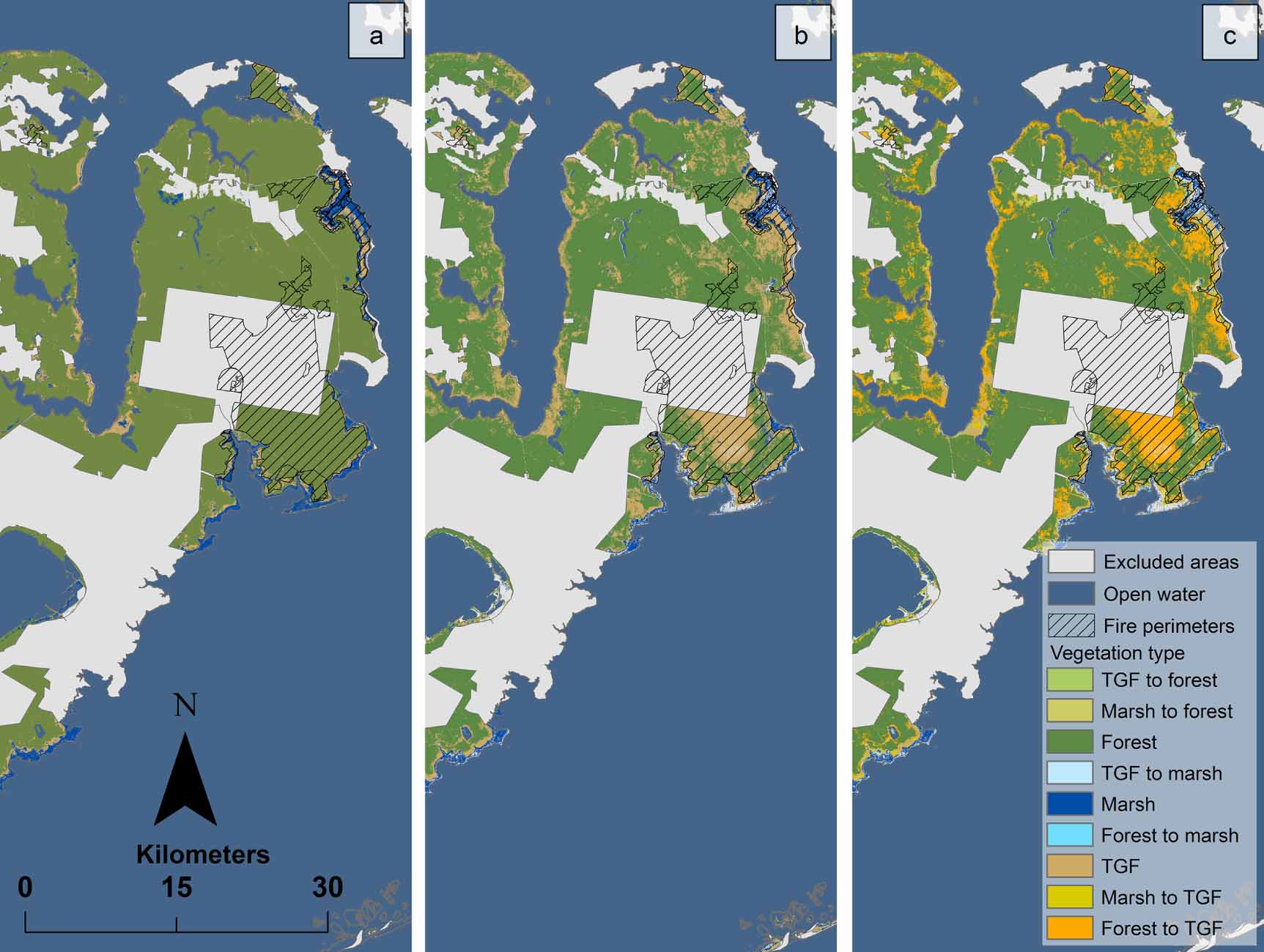
On unmanaged public lands not impacted by fire, there was a net loss of forest (152 km2) between 2001 and 2014, with 167 km2 of coastal forest converting to transition-ghost forest during this period; this change occurred on approximately 15% of the area. Conversion of transition-ghost forest to marsh comprised approximately 6 km2 (0.5%). Between 2001 and 2014, 81% of the study area remained in the same forest vegetation type (figure 3(c), see table S7 for error estimates).

Figure 3. (a) Vegetation classification (forest, transition-ghost forest as TGF, and marsh) of the eastern portion of the Albemarle-Pamlico Peninsula, NC in 2001; (b) vegetation classification of the eastern portion in 2014; and (c) vegetation class change between 2001 and 2014.
Download figure:
Standard image High-resolution image3.2. Measuring aboveground carbon
Total aboveground biomass models performed well, with the 2014 RF model performing slightly better (R2adj. = 0.78, RMSE = 15.0 Mg ha−1, % RMSE = 9.5) than the 2001 model (R2adj. = 0.75, RMSE = 18.3 Mg ha−1, % RMSE = 12.6) (figure S6). Mean and median vegetation height predictor variables contributed most to overall model performance, confirming the importance of vegetation structure to aboveground biomass estimation (figure S7). By vegetation type, predicted total aboveground biomass for the forested vegetation class (2001 R2adj. = 0.96, 2014 R2adj. = 0.92) outperformed the predicted AGB for the transition-ghost forest (2001 R2adj. = 0.73, 2014 R2adj. = 0.76, figure S9). Mapped aboveground biomass change between 2001 and 2014 accurately related to field-based estimates of aboveground biomass change between 2003 and 2016 (R2adj. = 0.64, RMSE = 13.4 Mg ha−1, figure S10).
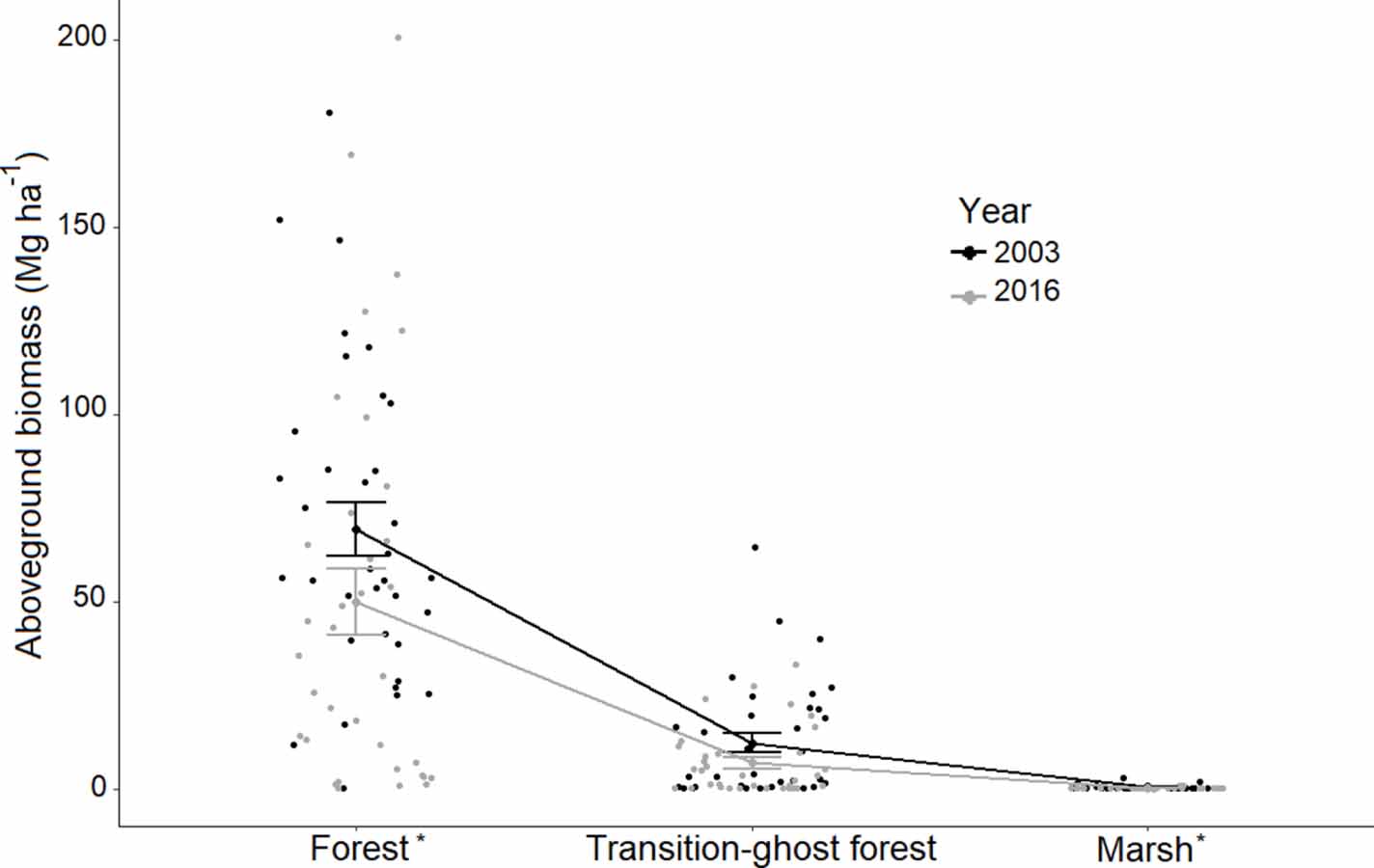
On unmanaged public lands not impacted by fire, change in AGB was positive (mean 10.7 ± 2.3 Mg ha−1) with a net of 1.21 ± 0.26 Tg (6.2 Tg in 2001; 7.4 Tg in 2014). This equates to a 19% increase (0.53 ± 0.10 TgC) in aboveground carbon stores between 2001 and 2014 (table 1). Though carbon gains offset declines, biomass dynamics varied spatially, with losses occurring closer to the estuarine shoreline and gains more prevalent inland (figure 4(a)). We confirmed significant aboveground biomass declines (Wilcoxon Signed Rank test, α = 0.05) in the field measurements during the study period (figure 5), with a total aboveground biomass loss overall of 8.8 ± 2.1 Mg ha−1 (p-value < 0.001); forest plots decreased in aboveground biomass by 28% (p-value < 0.05), and transition-ghost forest plots decreased by 39% (p-value = 0.2).
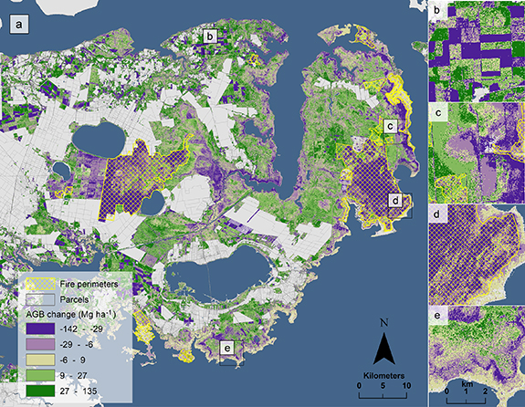
Figure 4. (a) Aboveground biomass change (AGB; measured in Mg ha−1) on the Albemarle-Pamlico Peninsula in eastern North Carolina, USA. Grey areas are unmeasured areas (non-forested in 2001, e.g. developed lands or agricultural areas) and yellow crosshatched areas are fire perimeters provided by the Monitoring Trends in Burn Severity (MTBS) dataset. (b) An example of AGB change resulting from human land-use activities like planting and harvesting on pine plantations. (c) An example of AGB change along the shoreline in an unmanaged public portion of the landscape. (d) AGB change within the fire perimeter of the Pains Bay fire that occurred in 2011. (e) Characteristic pattern of forest dieback resulting from either an acute or gradual saltwater intrusion event (within Gull Rock Game Lands).
Download figure:
Standard image High-resolution image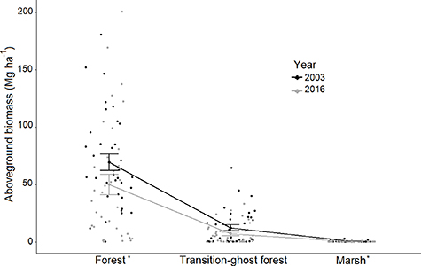
Figure 5. Mean field-measured aboveground biomass and associated standard errors (S.E.) by vegetation type (forest, transition-ghost forest, and marsh) and year (2003 = black, 2016 = light grey) for 98 plots distributed across 5 sites on the Albemarle-Pamlico Peninsula in eastern NC, USA. The * denotes a statistically significant difference between years using the Wilcoxon Signed Rank Test (p < 0.05). For more detailed marsh plots, see figure S11.
Download figure:
Standard image High-resolution imageTable 1. Measures of total area (km2), mean aboveground biomass (AGB) change (Mg ha−1), net aboveground biomass (Tg), and associated model standard errors (S.E.) for different landscape summary categories and for selected vegetation change classes for the Albemarle-Pamlico study area in eastern North Carolina, USA. In landscape category descriptions, '–' = 'excluding' and '+' = 'including'. Values for change classes are reported only for unmanaged public lands not including those impacted by fire.
| Total area | Mean AGB change (S.E.) | Net AGB (S.E.) | |
|---|---|---|---|
| Landscape category | |||
| Unmanaged public lands–fire | 1138 | 10.7 (2.3) | 1.21 (0.26) |
| Unmanaged public lands + fire | 1381 | 6.0 (2.2) | 0.83 (0.30) |
| Unmanaged public lands + private lands–fire | 3320 | 14.4 (2.4) | 4.67 (0.80) |
| Unmanaged public lands + private lands + fire | 3716 | 11.0 (2.3) | 3.96 (0.85) |
| Fire | 396 | −18.2 (1.3) | −0.71 (0.05) |
| Pains Bay fire | 160 | −16.7 (1.5) | −0.27 (0.02) |
| Evans Road fire | 165 | −24.2 (1.3) | −0.40 (0.02) |
| Change class | |||
| No change foresta | 828 | 17.8 (2.8) | 1.49 (0.23) |
| Forest to transition-ghost forest | 167 | −16.2 (1.1) | −0.27 (0.02) |
| No change transition-ghost forest | 39 | −7.3 (0.8) | −0.03 (0.003) |
| Transition-ghost forest to marsh | 6 | −7.2 (0.4) | −0.004 (0.0002) |
aIncluding unchanged forested private lands, net AGB is 4.90 ± 0.51 Tg (2.46 ± 0.25 TgC).
When the impacts of fire were included, AGB on unmanaged public lands only increased by 0.83 ± 0.30 Tg between 2001 and 2014, with mean 6.0 ± 2.2 Mg ha−1.
Without fire, AGB on unmanaged public lands plus private lands increased by 4.67 ± 0.80 Tg (mean 14.4 ± 2.4 Mg ha−1) between 2001 and 2014 but only increased by 3.96 ± 0.85 Tg (mean 11.0 ± 2.3 Mg ha−1) when the impacts of fire were included.
Fire disturbances alone resulted in an overall AGB loss of 0.71 ± 0.05 Tg (−0.35 ± 0.05 TgC; figure 6) between 2001 and 2014. The Pains Bay fire (2011) resulted in an AGB loss of 0.27 ± 0.02 Tg (figure 4(d)) and the Evans Road fire (2008) resulted in an AGB loss of 0.40 ± 0.02 Tg (table 1).
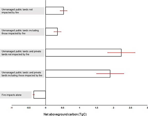
Figure 6. For the Albemarle-Pamlico Peninsula in eastern NC, USA, net aboveground carbon (TgC) and associated model standard errors summarized by: (1) unmanaged public lands not impacted by fire; (2) unmanaged public lands including those impacted by fire; (3) unmanaged public lands and private lands not impacted by fire; (4) unmanaged public lands and private lands including those impacted by fire; and (5) fire impacts alone.
Download figure:
Standard image High-resolution imageBy combining our vegetation class change maps from section 3.1 and AGB maps described above, we quantified between- and within-class changes in AGB (figure 7). Forested areas that remained forested between 2001 and 2014 experienced an overall net increase in AGB (17.8 ± 2.8 Mg ha−1, table 1). This resulted in an aboveground carbon gain of 0.75 ± 0.12 TgC (2.46 ± 0.25 TgC when private lands are included). Conversion from forest to transition-ghost forest resulted in AGB loss (−16.2 ± 1.1 Mg ha−1) and a 0.13 ± 0.01 TgC loss in aboveground carbon. Transition-ghost forest that remained transition-ghost forest experienced an overall net decline in aboveground biomass (−7.3 ± 0.8 Mg ha−1).

Figure 7. Violin plots of aboveground biomass change (sampled at 500-m intervals across unmanaged public lands not impacted by fire on the Albemarle-Pamlico Peninsula in eastern NC, USA) summarized by vegetation type change (transition-ghost forest abbreviated as TGF).
Download figure:
Standard image High-resolution image3.3. Salinity and aboveground carbon dynamics
Using distance from the estuarine shoreline as a proxy for sea level rise vulnerability, we observed that areas closer to the shore (<1 km) had a net negative AGB change (−2.6 ± 0.8 Mg ha−1), and areas farther from the shore (>1 km) had a net positive change (14.1 ± 0.9 Mg ha−1) in AGB (Kruskal-Wallis test; p-value < 0.0001). Our salinity interpolation ranged from 0 ppt to a maximum of 18 ppt in our study area (figure 8(b)), very similar to soil water measurements collected at the field sites (Taillie et al 2019). Using a threshold of 2 ppt (Herbert et al 2015), areas with lower salinities (<2 ppt) gained more aboveground biomass between 2001 and 2014 (gain = 30.7 ± 0.8 Mg ha−1) than areas with higher salinities (>2 ppt; gain = 12.8 ± 1.0 Mg ha−1; Kruskal-Wallis test; p-value < 0.0001).

Figure 8. (a) Euclidean distance to connected canals; inset = Euclidean distance to estuarine shoreline only. (b) Salinity interpolation, measured in parts per thousand (ppt), using the 40 water quality monitoring stations along the Albemarle and Pamlico Sounds in eastern North Carolina; inset = all points used in salinity interpolation from the Environmental Protection Agency's STORET database. High salinities occur along the estuarine shoreline in the east and gradually decrease westward, with increasing distance from the shoreline. High salinities also occur in the southern part of the peninsula, resulting from proximity to the more saline Pamlico Sound, with decreasing salinities northward closer to the near-fresh Albemarle Sound.
Download figure:
Standard image High-resolution image
Results from our spatial error model indicated that salinity was negatively related to aboveground biomass; as salinity increases AGB decreases (p-value < 0.01). Connected canal distance was also negatively related to aboveground biomass (p-value < 0.01). The effect of elevation on aboveground biomass differed based on the characteristic vegetation type present in 2014; elevation was positively related to aboveground biomass in the marsh and transition-ghost forest vegetation types but negatively related to aboveground biomass in areas classified as forest (table 2).
Table 2. Parameter estimates and standard errors ('S.E.') for the ordinary least squares (OLS) regression model and the spatial error model (SEM) to test the relationship between aboveground biomass change (Mg ha−1) and five potential drivers at 1000 random locations on the Albemarle-Pamlico Peninsula in NC, USA. Akaike information criterion (AIC), pseudo-R squared, and Moran's I residuals are also provided.
| OLS | SEM | |
|---|---|---|
| estimate (S.E.) | estimate (S.E.) | |
| (Intercept) | 38.0 (3.1)*** | 30.0 (4.6)*** |
| Salinity | −1.8 (0.4)*** | −1.7 (0.7)** |
| Distance to estuarine shoreline | 1.5 (0.5)** | 1.9 (0.9)* |
| Distance to connected canals | −3.9 (1.0)*** | −3.2 (1.4)** |
| Transition-ghost forest | −14.4 (23.2) | −20.8 (21.8) |
| Marsh | −46.2 (5.8)*** | −41.2 (5.5)*** |
| Elevation | −27.0 (4.7)*** | −24.7 (5.1)*** |
| Salinity: distance to estuarine shoreline | 0.1 (0.1) | 0.2 (0.2) |
| Transition-ghost forest: elevation | 13.3 (64.3) | 27.1 (59.6) |
| Marsh: elevation | 34.4 (10.0)*** | 31.0 (9.5)*** |
| AIC | 9313.7 | 9245.1 |
| Moran's I residual | 0.1*** | 0.0 |
| (Pseudo- R squared) | 0.27 | 0.32 |
Significance codes: 0 '***' 0.001 '**' 0.01 '*' 0.05 '.' 0.1 ' ' 1
4. Discussion
Our results highlight that, although aboveground carbon declines are apparent nearshore, land management activities and forest growth offset these declines. As the landward extent of sea level rise impact increases, this study highlights potential opportunities for targeted human interventions to preserve the region's carbon sink. Studies in highly dynamic coastal systems at fine scales across broad spatial extents are rare, posing challenges for monitoring and forecasting coastal ecosystem change. However, with increasing availability of data from aerial- and satellite-based LiDAR platforms, our methods can be applied in other low-lying coastal plains to develop landscape-scale measurements of historical impacts from sea level rise and identify areas most vulnerable to future impacts. Investigations at these large scales are requisite for allocating resources for monitoring, targeting interventions, and adapting to a changing environment.
Coastal vegetation transitions are driven by complex interactions between gradual climate changes and episodic disturbance events. Impacts from gradual inundation alone occur at long (e.g. centuries) temporal scales (Schieder et al 2018, Schieder and Kirwan 2019). At much shorter time scales (such as the one evaluated in this study), it is more likely for episodic disturbances to drive vegetation changes (Poulter et al 2009). However, the frequency, extent, and severity of disturbances can be exacerbated or mediated by climate change (Bender et al 2010). Droughts, as an example, are expected to increase in duration and severity as the climate changes, increasing saltwater exposure in freshwater ecosystems (via landward movement of the freshwater-saltwater interface) (Ardón et al 2016). These complex interactions (Herbert et al 2015), in addition to land-use impediments like upslope agricultural fields or urban development (Enwright et al 2016, Borchert et al 2018), will ultimately determine the spatiotemporal patterns of forest retreat in coastal systems.
Between 2001 and 2014, we measured conversion from forest to a short (<5 m) shrub-dominated transition phase on 15% of unmanaged public lands in our study area. Analyzing temporal shifts in species composition using the same field plots as this study, Taillie et al (2019) confirmed low tree regeneration between 2003 and 2016. Corroborating previous field studies (Raabe and Stumpf 2016, Langston et al 2017), their results indicated a general shift in vegetation towards more salt-tolerant shrubs and herbaceous vegetation over the course of the study (Taillie et al 2019). From our regression models, we identified differential impacts of elevation on aboveground biomass across vegetation types. The counterintuitive result for forests (a negative relationship between forest aboveground biomass and elevation) may reflect the inclusion of unknown human land-use management on public lands affecting forest structure and species composition and/or drainage patterns. It may also reflect the overall decrease in aboveground biomass variability as elevation increases or the transition into a forest class with lower aboveground biomass. Both our spatial predictions and regression models indicated that aboveground biomass and carbon declines were more likely near the estuarine shoreline and in areas with higher salinities. This supports other studies that have demonstrated the importance of salinization as a stronger driver of coastal forest change than elevation and inundation alone (Krauss et al 2007, Craft 2012, Taillie et al 2019). Shorelines, creeks, and artificial drainages can serve as conduits for saltwater to move inland, causing forest dieback in areas proximal to these landscape features (Herbert et al 2015, Krauss et al 2018, Ury et al 2020).
Human activities on private lands at higher elevations in the study area resulted in heterogeneous patterns of both aboveground carbon gains and declines. However, their net contribution to aboveground carbon storage was positive. Carbon dynamics on private lands in the study area result from individual land-use decisions, including planting and harvesting of timber and hydrologic modification via artificial drainages and canals. Though meant to move water off lands, the extensive drainage networks in our study area are also susceptible to saltwater intrusion from gradual inundation and hurricanes (Manda et al 2014; Bhattachan et al 2018). The efficacy of the networks is highly dependent upon landowner management (Poulter et al 2008). Our spatial regression model showed that, on unmanaged public lands, aboveground biomass declines were more prevalent farther from drainage networks. This may seem counterintuitive, but it is possible that active management of drainage networks on public lands has lessened the extent of saltwater intrusion. On private lands, the relationship between biomass and canals might differ because landowner objectives and resources may not match those of public land managers. To prevent net carbon loss associated with climate change and sea level rise, opportunities exist on private lands to increase carbon through management activities like reforestation, lengthened harvest cycles, and restricting harvests. These land management decisions also have numerous co-benefits including increases in water availability and biodiversity (Law et al 2018). Human land management decisions and interventions on the Albemarle-Pamlico Peninsula will largely determine the continued ability of the region to serve as a carbon sink.
Fire disturbance may also facilitate the progression from forest to marsh on salt-affected lands. Frequent, low-intensity fires have historically maintained vegetation structure in these coastal ecosystems (Frost 1995, Poulter et al 2009). Post-fire, we would expect to see regeneration as part of natural forest succession. Comparing two catastrophic wildfires that occurred during our study period—one in 2008 (Evans Road fire) in the study area center and another in 2011 (Pains Bay fire) near the estuarine shoreline—we find less regeneration than expected (Frost 1995), as indicated by the aboveground carbon estimates, within the fire perimeters near the shoreline. Fire disturbance and saltwater intrusion may have an interactive effect that inhibits woody species growth and promotes marsh migration landward. Seedlings and saplings of freshwater woody species need sufficient time to establish post-fire, but if saltwater exposure occurs before these saplings have established, post-fire regeneration will be reduced (Poulter et al 2008). Although fires have historically played a significant role in maintaining vegetation structure and composition in this region, this role may be changing along with the changing climate.
Saltwater intrusion from sea level rise is often considered an 'invisible' threat because shifts in soil chemistry are difficult to measure at large spatial scales and are not generally perceived by the public (Tully et al 2019). However, ghost forests provide clear markers of sea level rise's leading edge. There is still a great deal of uncertainty about system-level impacts of salinization on net carbon (Henman and Poulter 2008), with recent research highlighting divergent biogeochemical responses of soils to saltwater intrusion (Ardón et al 2013, Herbert et al 2015, Helton et al 2019). Future work that quantifies the landscape-scale impacts of saltwater intrusion on different carbon pools, would complement our estimates of aboveground carbon. As rates of sea level rise accelerate and the landward extent of impact increases, a better understanding of the spatiotemporal patterns of forest retreat and aboveground carbon in coastal systems is essential for developing effective management and adaptation plans. Our research provides a critical baseline, from which policy makers, landowners, and managers can draw, to better anticipate the interventions and adaptation activities necessary in both the near- and far-term.
Acknowledgments
We are grateful to Dr Megan Skrip from the Center for Geospatial Analytics for edits and comments that greatly improved the quality of this manuscript. We thank Dr Vaclav Petras of NC State University, who provided technical insights and troubleshooting during the LiDAR data processing phase in GRASS GIS. Additionally, Douglas Newcomb of the U.S. Fish and Wildlife Service, provided valuable comments on methods and analyses. Finally, we thank the three anonymous reviewers whose comments greatly improved this manuscript.
Funding
This research was funded by a joint fellowship through NOAA's North Carolina Sea Grant Program and NASA's North Carolina Space Grant Program (NOAA award # NA14OAR4170073, NASA award # NNX15AH81H). Funding from a College of Natural Resources Innovation Grant at NC State University was also used to support this research.
Conflicts of interest
The authors declare no conflict of interest.