


Introduction
The value of statistical life (VSL) is the marginal willingness to pay for (or the marginal willingness to accept) marginal risk reductions in a given context (environmental pollution, road safety, and occupational safety, among others), but it does not correspond to the ex-post value of the saved lives. Although from ethical and moral points of view, for many people, making an estimate of this type is questionable, in reality, there are certain situations in which this value is indeed quantified, particularly those in which individuals are willing to accept greater or lesser exposure to risk due to the tradeoff between the risk of mortality and money (Reference Gentry and ViscusiGentry and Viscusi 2016). For example, this value is useful for the cost-benefit analysis of projects that may aim to reduce levels of accidents, illness, or mortality. Therefore, having an estimate of VSL contributes greatly to decision-making, especially in low-income countries, where such studies are typically not performed (Hammitt and Robinson 2007).
The most commonly used approaches to quantifying VSL are the revealed preference approach, typically known as the hedonic wage method (which uses labor market information to relate the level of remuneration and the risk to which workers are exposed), and the stated preference approach (in which people are asked directly through surveys their willingness to pay for different hypothetical reductions in the level of risk). According to Viscusi and Aldy (Reference Viscusi and Aldy2003), most studies in the United States are based on labor market information using the hedonic wage method, whereas in Europe, the emphasis is on using the stated preference approach. Most hedonic wage studies use cross-sectional data; however, recently, the use of panel data (Reference Schaffner and SpenglerSchaffner and Spengler 2010) has been emphasized, in addition to some other aspects, such as making differential estimates of VSL by type of risk (Reference Scotton and TaylorScotton and Taylor 2011) or according to age groups (Reference Evans and SchaurEvans and Schaur 2010), as well as the disaggregation of risk by industry and occupation (Reference Riera Font, Penalva and SbertRiera Font, Ripoll Penalva, and Sbert 2007).
In many developing countries, the information needed to use one of these methods is not available, so a good alternative approach for the VSL is to extrapolate estimates from other countries (mainly developed) by relating the VSL to the GDP per capita of each country. For example, through a meta-analysis, Miller (Reference Miller2000) estimates a VSL of US$1.2 million for Argentina, US$0.7 million for Brazil, US$0.7 million for Chile, US$0.4 million for Peru, US$0.8 million for Uruguay and US$0.5 million for Venezuela (all values correspond to 1995 dollars). Lindhjem et al. (Reference Lindhjem, Navrud, Braathen and Biausque2011) performed a meta-analysis using previous VSL estimates for thirty-eight countries (all included values using the declared preference approach). These authors report an average VSL of US$6.0 million. When classified according to the context of the study, the average VSL correspond to US$9.0 million for environmental pollution, US$6.9 million for road safety and US$4.0 million for health.
In the case of Chile, some studies use the stated preference approach, but only one previous study uses the hedonic wage method. This last study was carried out by Parada-Contzen, Riquelme-Won, and Vasquez-Lavin (Reference Parada-Contzen, Riquelme-Won and Vasquez-Lavin2013), who estimate a VSL of US$12.8 million after correcting for endogeneity and selection bias. This estimate is quite high in comparison to other developing countries and even higher than in some developed countries.Footnote 1 This situation is not unusual because, although the concept of the value of statistical life is well established and widely used in economics, there is still controversy over the apparent instability in estimates of excessively large or small values (Reference Viscusi and AldyViscusi and Aldy 2003). In this sense, some theoretical studies have noted that the potential bias of the estimates arises due to omitted variables (Reference Hwang, Reed and HubbardHwang, Reed, and Hubbard 1992; Reference Shogren and StamlandShogren and Stamland 2002). From an empirical perspective, Kniesner et al. (Reference Kniesner, Viscusi, Woock and Ziliak2007) demonstrate how the use of the best available data (panel data and risk level with high disaggregation) and the best econometric practices can determine the estimated VSL in previous studies.Footnote 2
This situation motivated the realization of the present study, which uses more updated data with more explanatory variables and new instrumental variables to provide new evidence to clarify if the VSL for Chile estimated with the hedonic wage method is significantly different from the value of other countries with similar GDPs per capita and if the result of the only previous study can be attributed to data and/or methodological problems. Specifically, the contribution of this paper is in the line of demonstrating that the use of relevant instrumental variablesFootnote 3 that meet the exogeneity requirement makes it possible to correct for the problem of the endogeneity of risk and to improve the previous VSL estimates for the case of Chile.
Methodology
Econometric framework
When the available information is cross-sectional, the hedonic price method uses a linear regression, which represents the relationship between the wage level and the explanatory variables. The general model is as follows:

where ln(wi) is the natural logarithm of the wage, H corresponds to the vector of personal characteristics, Ji represents the vector of the characteristics of the work, Li represents the vector of the characteristics of the firm, Gi represents the vector of geographical variables, ri corresponds to fatal risk, and pi corresponds to nonfatal risk. In turn, the vectors β, α, θ, and δ and the scalars c, γ and τ correspond to the parameters estimated in the regression, whereas ei is the error term. The subscript i indicates that the information corresponds to the i-th individual.
However, if there are unobservable variables that are correlated with one of the variables included in the statistical model (for example, risk aversion is not an observable variable for the researcher), the parameters estimated by the ordinary least squares method (OLS) will be biased and inconsistent. In relation to labor risk variables, what is relevant is not the risk to which the individual is exposed but the individual’s perception of the risk. This is why in the literature, the use of instrumental variables is suggested to estimate the perceived risk of individuals related to their work, which would reduce bias and inconsistency due to endogeneity.
If there are several instrumental variables to correct the endogeneity of one or several explanatory variables, the method of least squares in two stages (2SLS) can be used. In the first stage, the predicted values of the endogenous explanatory variables (ri and pi) are obtained from a regression related with the other exogenous explanatory variables and the instrumental variables. In the second step, a regression is generated through the OLS method of the variable ln(wi) with respect to the exogenous explanatory variables and the estimated values of the endogenous explanatory variables. Specifically, in this case, the predicted value of nonfatal and fatal risk can be obtained with the following regressions:


where Si is a vector of instrumental variables that determine the risk of the individual, c 1 and c 2 are constants, ς, σ, χ, ψ and φ 1 correspond to the parameter vectors estimated for the nonfatal risk regression, and ω, ξ, ϑ, κ, and φ 2 correspond to the parameter vectors estimated for the fatal risk regression. Finally, μi and vi correspond to the random errors of the respective regressions.
Another problem related to the nature of cross-sectional data in studies to estimate the VSL is the so-called selection bias, which arises when the sample used to perform the regression is not completely random. The problem is that it is intended to estimate the wage offer equation for “all” individuals of working age, regardless of whether the individual is working. However, data related to the wage offer are observable only for those individuals who are currently working. To solve this problem, Heckman (Reference Heckman1979) proposed a method known as Heckit, which proposes a regression model that consists of two related equations to correct the bias due to the self-selection of the sample.


where the latent variable  is greater than zero if the labor offer is observed in the data (yi = 1) or less than zero otherwise (yi = 0). Furthermore, it is assumed that the errors ei and ηi have a bivariate normal distribution. From these assumptions, it can be shown that the expectation of conditional equation (5) to which labor participation is observed is as follows:


φ(⋅) corresponds to the probability density function and Φ(⋅) refers to the cumulative distribution function, both estimated with a Probit model. In addition, for simplicity, the coefficient ρσe can be called βλ because it is the coefficient that accompanies the estimate of the inverse Mills ratio, λi. Rearranging equation (6) yields the following:

Once the model is presented, the estimation of the parameters of interest is carried out with a two-step procedure or with maximum likelihood routines.
Additionally, instrumental variables can be included to estimate if some of the explanatory variables are assumed to be endogenous. In this case, the procedure is known as Heckit in two stages with endogenous variables (Heckit 2SLS).
Data description
From the review of several studies of hedonic salaries published in the last two decades, it was possible to determine the explanatory variables that are commonly included in this type of regressions.
As seen in Table 1, several categories of variables associated with personal characteristics, the characteristics of firms, labor information, and geographic variables are included. In the case of Chile, these variables are obtained from the CASEN survey performed in 2013.Footnote 4
Table 1 Variables used in published studies of hedonic wages to estimate VSL at the international level.

Source: Own elaboration.
It is also necessary to include variables associated with labor risk (fatal and nonfatal), which in Chile can be obtained from the records of the Social Security Superintendence (Superintendencia de Seguridad Social). According to data from 2013, the sectors with the highest mortality rate are mining (19.5 per 10,000 workers), transport and communications (17.5 per 10,000 workers), and construction (10.3 per 10,000 workers), whereas the sectors with the highest levels of labor accidents are the manufacturing (6.2 per 100 workers), transport and communications (6.0 per 100 workers), and agriculture (5.4 per 100 workers). In addition, the sector with the lowest accident rate is mining (1.6 per 100 workers).
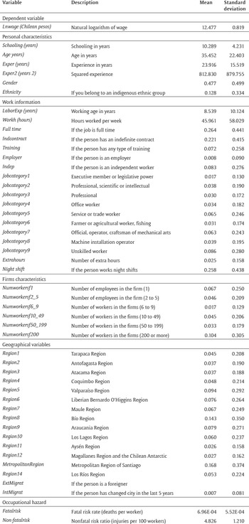
Table 2 presents the description of all the explanatory variables included in the present research.
Table 2 Description of variables.

Source: Own elaboration based on the CASEN Survey (2013) and Social Security Superintendence.
Moreover, it is necessary to incorporate instrumental variables to solve the problem of the endogeneity of labor risk (fatal and nonfatal).
According to Garen (Reference Garen1988), the instrumental variables that should be included in this type of study correspond to the nonlabor income and factors correlated with the perceived risk in the work but that do not explain the wage (see Table 3). Therefore, variables include: a dummy variable that takes a value of 1 if the partner of the individual has some type of disability (Disabhome), the nonlabor income in Chilean pesos (Nonlabincome), the number of children under six years of age (Numberkids6), a variable that determines the interaction between gender and children under six years old (Genderkids6), a dummy variable that takes a value of 1 if the individual is married (Married), the years of schooling of the couple (Coupleschooling), a dummy variable that takes a value of 1 if the individual’s partner works (Coupleworks), the number of people who are economically dependent on the household (Peoplehome), a dummy variable that takes a value of 1 if the individual has a life insurance (Lifeinsurance), and another dummy variable that takes a value of 1 if the individual lives with his partner, regardless of whether he is married (Withcouple). These are proxy variables of risk aversion that can affect the desire to have a safer job.
Table 3 Description of instrumental variables.

Source: CASEN Survey (2013) and Ministry of Economy.
Note: The variables with units not specified correspond to the proportion of membership, which is defined by a dichotomous variable that takes a value of 0 or 1, where 1 implies membership and 0 implies nonmembership.
In addition, Angrist and Krueger (Reference Angrist and Krueger2001) state that the inclusion of labor market variables is a useful way to achieve identification with the method of instrumental variables. For this reason, the proportion of firms by size by economic sector is considered as instruments, considering small firms (VI_smallfirms), medium firms (VI_mediumfirms), and large firms (VI_largefirms); in this case, micro firms are the control group. These variables are included because in Chile, a relationship has been observed between the size of the firms and the rate of labor accidents,Footnote 5 they reflect the characteristics of the labor market, and the workers in economic sectors with a greater proportion of small firms could have less bargaining power to alter their wages, so it is assumed that the requirement of exogeneity would be met.
Estimation of VSL
After estimating the parameters in the regressions, it is possible to calculate the VSL for Chile with the following equation:

where  corresponds to the average monthly wage, which is multiplied by 12 to obtain the annual average wage, and γ corresponds to the estimated parameter of the fatal risk. In addition, to make the results of this study comparable with previously published international estimates, conversion of values to 2013 dollars is performed.
Transfer of benefits from VSL
The empirical literature for developing countries is scarce in this area, so there are no estimates for individual countries. This has led to suggesting the transfer of the VSLs from countries with estimates to countries that do not have them. The most common approach to transfer benefits is to assume that the ratio of VSL relative to GDP per capita is constant across countries, which implies assuming an income elasticity equal of 1.0. However, recent studies state that an income elasticity equal to 1.0 may be inadequate for low-income countries, so Hammitt and Robinson (Reference Hammitt and Robinson2011) suggest using an income elasticity of 1.5 to provide a range of values for VSLs in countries of low and middle incomes. Another approach to extrapolate the results is to relate the VSL to each country’s GDP per capita by performing a meta-analysis (see Reference MillerMiller 2000; Reference De Blaeij, Florax, Rietveld and VerhoefDe Blaeij et al. 2003; Reference Bellavance, Dionne and LebeauBellavance, Dionne, and Lebeau 2009; Reference Hammitt and RobinsonHammitt and Robinson 2011).
Therefore, after estimating the VSL for Chile, this value will be included along with estimates previously published in scientific journals for different countries that also use the hedonic wage approach in order to extrapolate the VSL for other Latin American countries.
Results
Estimation of the VSL for Chile
Different statistical methods were used to estimate the VSL for Chile (OLS, 2SLS, Heckit, and Heckit 2SLS).Footnote 6 Most of the estimated parameters are significant at 1 percent, except for certain dichotomous variables related to firm size, type of occupation, and geographical variables. Moreover, the coefficients related to schooling, experience, training, and contract type show expected magnitudes and signs in relation to what the theory postulates and what has been observed in other studies of hedonic wages. In particular, the estimated coefficient for the educational variable has a magnitude between 0.037 and 0.049, which would indicate that one year of schooling increases wages approximately between 3.7 percent and 4.9 percent. Another variable to be highlighted is gender, which was positive in the estimates that did not correct for selection bias; this would indicate that men earn between 25.9 percent and 31.9 percent more than women. However, this gap is reduced (between 15.2 percent and 20.6 percent) when estimating the Heckit and Heckit 2SLS models, which correct the selection bias associated with women tending to participate less in the labor market.
In relation to the fatal risk parameter, this proved to be positive and significant at 1 percent in all estimates. However, there is a considerable difference in the estimated magnitudes; for example, the parameters estimated through the OLS and Heckit were found to be less than one third of the values estimated through the 2SLS and Heckit 2SLS method.
In contrast, the parameter of nonfatal risk was found to be significant in all the estimates, with a negative sign, contrary to what was expected. However, this result is also observed in other studies such as Riera Font, Ripoll Penalva, and Sbert (Reference Riera Font, Penalva and Sbert2007) and Arabsheibani and Marin (Reference Arabsheibani and Marin2000). In this case, the negative sign could be attributed to the fact that in Chile, the mining sector pays the highest average wages and presents a high fatal risk but also less nonfatal risk with respect to other economic sectors. Furthermore, nonfatal risk data may not be totally useful in this kind of estimation, even with better instrumental variables, because typically in official statistics serious accidents are presented together with nonserious ones.
At the same time, it can be observed that in the 2SLS and Heckit 2SLS estimates most of the estimated parameters are not sensitive to the inclusion of instrumental variables, except the coefficients associated with the variables related to fatal and nonfatal risk. In addition, the RFootnote 2 values calculated are similar, with a magnitude close to 0.45, which is common in hedonic wage studies.
In the case of estimates with instrumental variables, their validity must be tested because the stronger the relationship between an instrumental variable and the endogenous explanatory variable(s) are, the better the instrument is. In addition, it is required that the instrumental variable is not correlated with other variables that affect the outcome (exogenous condition). These requirements ensure that the instrument can estimate parameters in an unbiased and consistent way.
Most of the included instrumental variables were significant at 1 percent or 5 percent, but only the instrument inclusion related to the proportion of firms by size according to economic sector significantly improved the regression adjustments for the variables of fatal risk (R2 = 0.43) and nonfatal risks (R2 = 0.45). This is important because if the instruments are poorly correlated with the endogenous explanatory variable, the parameters estimated by the 2SLS method may be even worse than using the OLS method. If there is only one endogenous regressor variable and the instrumental variables have an F test value close to or less than 10, it should be considered as a weak instrument group according to a finger rule established by Staiger and Stock (Reference Staiger and Stock1997). This was corrected by Stock and Yogo (Reference Stock and Yogo2005), who simulated critical values to detect weak instruments under multiple endogenous explanatory variables using a Wald test based on the Cragg-Donald statistic.
In replicating the study by Parada-Contzen, Riquelme-Won, and Vasquez-Lavin (Reference Parada-Contzen, Riquelme-Won and Vasquez-Lavin2013) with data from CASEN 2013, the value of the test proposed by Stock and Yogo (Reference Stock and Yogo2005) is lower than the critical value, so the hypothesis of weak instruments cannot be rejected. In contrast, if the instruments used in the present study are considered, the values of the tests in the 2SLS and Heckit 2SLS models are much higher than the critical value, which is why the hypothesis of weak instruments is rejected in this case.
Regarding the exogeneity condition, only three of the instrumental variables proposed in this study fulfilled the Hansen J test, which evaluates partial exogeneity. These instrumental variables were the number of people who are economically dependent on the household, the proportion of large firms by economic sector and the proportion of small firms by economic sector. Consequently, the inclusion of these three instruments meets the requirements of relevance and exogeneity required by the method of instrumental variables; therefore, they were the only ones used in the regressions reported in Table 4. While replicating the study of Parada-Contzen, Riquelme-Won, and Vasquez-Lavin (Reference Parada-Contzen, Riquelme-Won and Vasquez-Lavin2013) with the data from CASEN 2013, the value of the J test is high, rejecting the hypothesis of partial exogeneity of the instrumental variables included in that study.
Table 4 Results according to the estimation method.
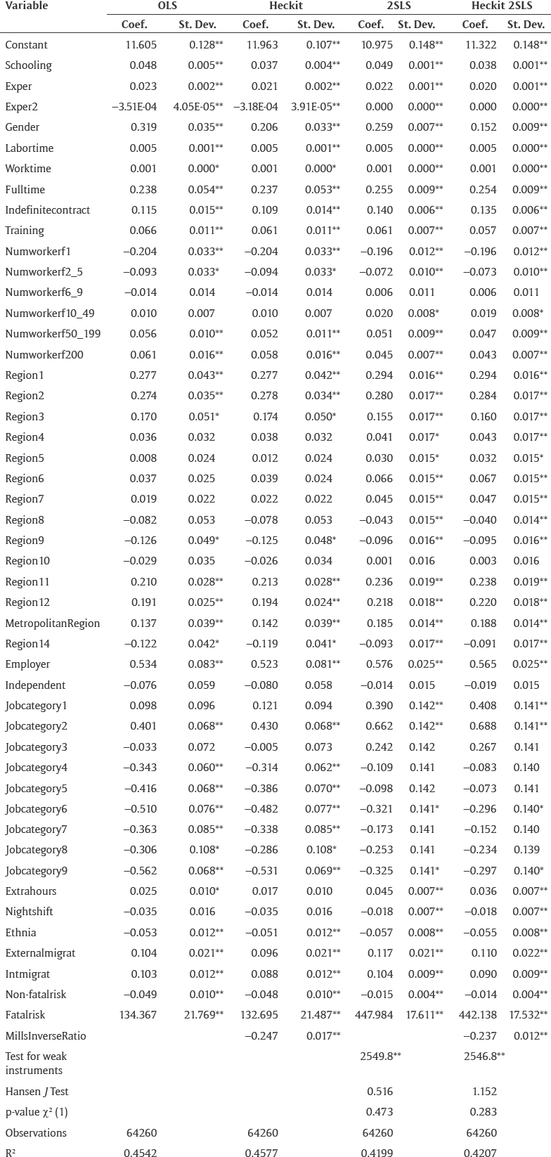
Source: Own elaboration.
Note: **significant at 1%, *significant at 5%.
From the tests performed, it is concluded that the instrumental variables used by Parada-Contzen, Riquelme-Won, and Vasquez-Lavin (Reference Parada-Contzen, Riquelme-Won and Vasquez-Lavin2013) correspond to weak instruments and do not meet the requirement of exogeneity. Therefore, the parameters estimated through the 2SLS method based on these instruments would be biased and inconsistent, which would explain the high value of the VSL for Chile estimated by that study compared to other estimates for countries with similar GDPs per capita.Footnote 7 In contrast, the three instrumental variables used in this study meet the relevance and exogeneity requirements, which validates the estimates made by the 2SLS and Heckit 2SLS methods. However, because we detected the presence of a selection bias (significant inverse Mills ratio variable in the Heckit regression), the best statistical model is Heckit 2SLS, which delivers a VSL of US$3.73 million (see Table 5).Footnote 8
Table 5 Estimation of VSL for Chile (millions of US$ year 2013).

Source: Own elaboration.
Lindhjem et al. (Reference Lindhjem, Navrud, Braathen and Biausque2011) mention that it is not appropriate to compare estimates of the VSL obtained through different approaches. However, for illustrative purposes only, Table 6 presents previous estimates made in Chile using the declared preference approach.
Table 6 Estimates of VSL for Chile with the stated preference approach.

Source: Own elaboration.
Most of all, the estimates obtained through the declared preference approach are several times smaller than those estimated through the revealed preference approach estimated in this study, which contradicts the results found by De Blaeij et al. (Reference De Blaeij, Florax, Rietveld and Verhoef2003). The lowest VSLs were published in scientific journals, whereas the highest VSLs were estimated in a report by GreenLab (Reference GreenLab2014) developed for the Chilean Ministry of the Environment. In addition, it is observed that none of the estimates with stated preferences are found in the confidence intervals reported in Table 6.
Extrapolation of VSL for Latin America
In this section, the available estimates for performing a meta-analysis and extrapolating the VSL for different countries in Latin America are reviewed. For this, the results of previous studies that use the hedonic wage method published in scientific journals are used, including the estimated VSL for Chile in this research.
To determine the relationship between the GDP per capita and VSL for each country, linear and logarithmic regressions were estimated. The regression with the least mean square error was as follows:

Thus, equation (10) was used to generate the VSL extrapolations for the different countries of Latin America, using the GDP per capita from 2013 of each country reported by the World Bank (see Table 7).
Table 7 GDP per capita and VSL estimated by study in 2013 dollars.
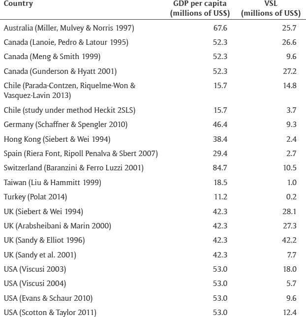
Source: Own elaboration.
The results of Table 8 show that the estimated VSL for Chile from the meta-analysis is lower than the VSL estimated in this study using instrumental variables (2SLS or Heckit 2SLS). It could be explained because meta-analysis does not include many observations from developing countries. In consequence, the results show the importance of performing empirical studies with micro-data in each country to have more accurate estimates In addition, Chile has the third highest estimated VSL based on the meta-analysis approach, behind Puerto Rico and Uruguay, which have estimated VSLs of US$5.20 million and US$2.18 million, respectively. In contrast, the lowest VSL is presented by Haiti, which amounts to US$0.01 million, followed by Nicaragua, Honduras, and Bolivia, which have values of US$0.06 million, US$0.09 million, and US$0.12 million, respectively.
Table 8 VSL estimation for Latin American countries.

Source: Own elaboration.
*Venezuela’s per capita GDP corresponds to 2012, because there are no records after that year.
The results of the meta-analysis carried out in this study provide evidence to suggest an income elasticity higher than 1.6, which agrees with recent studies that suggest the use of elasticities greater than 1, especially when results are extrapolated to low-income countries (Reference Hammitt and RobinsonHammitt and Robinson 2011).
Conclusions
In this study, we obtain the value of a statistical life in Chile using labor market information under different estimation methods to later calculate the VSL for different countries of Latin America through a meta-analysis.
Estimates for Chile with labor market data at the individual level are approximately double the values obtained by extrapolating the VSL from other studies of hedonic wages for countries with a similar GDP per capita. This shows the importance of performing empirical studies in each country to have more accurate estimates. In particular, the Heckit 2SLS method presented a VSL value of US$3.73 million (between US$3.44 million and US$4.02 million with a 95 percent confidence interval). It should be noted that the use of instrumental variables with weak instrument tests and partial exogeneity was validated, so the estimated parameters should be consistent despite the endogeneity of explanatory variables associated with fatal and nonfatal risk.
Additionally, from the meta-analysis, the VSL is obtained for each Latin American country, with an average value of US$0.82 million for this region. In addition, it is concluded that before an increase of GDP per capita of 1 percent per year, the VSL would grow by 1.64 percent.
Despite the low amount of data available to perform the meta-analysis and the fact that the scarcity of studies for low- and middle-income countries limits the extrapolation of VSLs for Latin American countries, the results obtained in this study could be an acceptable proxy in relation to the value of statistical life, considering that there are many countries in Latin America that do not have their own VSL estimates and that this information would allow for better decision-making in projects that directly or indirectly involve changes in the mortality risk of people.


 Open access