Intercomparison of Approaches to the Empirical Line Method for Vicarious Hyperspectral Reflectance Calibration

Introduction

The empirical line method (ELM) is well-recognized as an accurate, operational approach for the calibration of aerial and satellite imaging systems to correct multispectral and hyperspectral data from raw digital numbers (DNs) or radiance to at-surface reflectance factors (e.g., Ferrier and Trahair, 1995; Smith and Milton, 1999). If two or more ground targets with a known reflectance factor are placed within a scene, calibration for each spectral band reduces to an uncomplicated process of regressing the observed radiance against the known reflectance factor values. Linearity has been empirically demonstrated to be valid over the full range of low to high reflectance factor targets (Baugh and Groeneveld, 2008). The result is the calculation of gain and offset coefficients that can be applied to all surfaces in the scene, assuming uniform atmospheric conditions. The gain characterizes the sensor response of reflectance factor per unit radiance and the offset characterizes the sky path radiance between the sensor and the surface for a sensor system calibrated to radiance.

As part of a collaborative Cyanobacterial Harmful Algal Bloom (CyanoHAB) monitoring program in the Western Basin of Lake Erie (Figure 1) and Sandusky Bay, OH conducted from 2014 to present, we have developed and implemented an approach to apply an empirical atmospheric correction and vicarious reflectance factor calibration to the second generation, National Aeronautics and Space Administration (NASA) John Glenn Research Center's Hyperspectral Imager (HSI2). This manuscript focuses on methods developed at Kent State University (KSU) compared with those employed at Michigan Technological Research Institute (MTRI) and the University of Toledo (UT). Research conducted by MTRI, UT and other collaborators will be presented in greater detail separately. The HSI2 is an aerial imaging spectroradiometer that generates a hyperspectral datacube over the VNIR from 400 to 900 nm. Atmospheric correction is a necessary pre-processing step required prior to further processing to extract information about algal composition from the HSI2 image swaths (Gordon et al., 1988; Gao et al., 2009; Goetz, 2009). For the application presented in this study, the ELM is applied in four ways as described below. Three versions are simplified further to a single-point calibration by assuming that since the NASA Glenn S3 Viking aircraft carrying the spectroradiometer is flying at a low altitude that the path radiance between the surface and aircraft can be assumed to be negligible. The result may introduce an offset in the retrieved spectra compared to the actual surface spectrum, however the general spectral shape of the upwelling surface reflectance factor spectrum is still revealed (Farrand et al., 1994). This allows spectral shape based methods, which are not strongly dependent on absolute reflectance factor values to be effectively employed. The approach that we use here is the KSU visible derivative, Varimax-rotated, Principle Component Analysis (VPCA) spectral decomposition method, (Ali et al., 2013; Ortiz et al., 2013). Our conceptual approach also capitalizes on an innovative reflectance factor reference target, allowing the ELM to be applied directly to observations collected on the lake surface, which is the surface of particular interest for this and other aquatic studies. Application of these methods to the optically complex waters of Lake Erie is a stringent test of the approach because we document its applicability in highly turbid waters. The methods developed here will be applicable in coastal and inland water as well as marine environments imaged by proposed orbital hyperspectral missions such as the: Plankton, Aerosol, Cloud, ocean Ecosystem (PACE) mission, the Hyperspectral Infrared Imager (HyspIRI) mission, and the Geostationary Coastal and Air Pollution Events (GeoCAPE) mission. Deploying these orbital tools will create the opportunity for enhanced estimation of pigment-related biomass and new capabilities to identify algal and cyanobacterial composition based on extraction of pigment spectra by visible derivative spectroscopy.

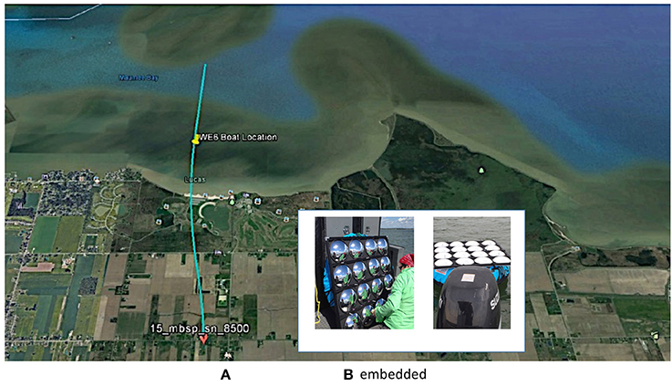
Figure 1. (A) Maumee Bay State Park is the location where the NASA Glenn, second generation Hyperspectral imager (HSI2) swath 15_MBSP was collected on June 21, 2016. Sampling station Western Erie 6 (WE6) is indicated, where measurements were taken from the boat, and the mirror array was deployed. (B) Inset: mirror calibration panel being cleaned on deck and deployed behind the vessel in Sandusky Bay (After Figure 4.3 with modification, Lekki et al., 2017).

Methods

The innovative calibration approach is to employ a floating panel (1.07 m by 1.17 m; 1.25 m²) composed of 16 convex mirrors (0.26 m diameter with radius of curvature 0.18 m) deployed on the water surface, providing an in-scene lake surface reference for image reflectance factor calibration. The convex mirrors reflect the direct sunlight and hemispherical sky illumination downwelling to the surface of the Earth back up to the HSI2 sensor while it is flying over the target. We can then use the HSI2 response of the mirror targets to normalize the upwelling radiance to percent reflectance factor, if we know the correct calibration gain function for the mirror target that transforms the HSI2 measured at-sensor radiance to a Lambertian surface reflectance factor. This effectively converts the spectroradiometer to a spectrophotometer merely by sacrificing a few scene pixels. An advantage of using convex mirrors deployed on the lake (Figure 1) is that their spherical surface produces a constant reflectance factor even when bobbing around on the unstable water surface. We have constructed a series of mirror panels for in scene reflectance factor calibration (Figure 1B). These were deployed as floating platforms in the western basin, Sandusky Bay, and a coastal transect along the southern shore of the central basin of Lake Erie using Ohio Division of Natural Resources (ODNR), United States Geological Survey (USGS), or Ohio Sea Grant vessels used as part of regular sampling trips conducted during NASA coincident over flights.

Ground-Based Measurements and Sampling

The image swath analyzed here was collected in the western basin of Lake Erie perpendicular to the coast over Maumee Bay State Park (MBSP), Oregon, OH, one of the surface calibration sites employed in the Lake Erie CyanoHAB monitoring program and includes the offshore sampling station designated WE6 (or sometimes WLE06) shown in Figure 1.

Each field site was revisited bi-weekly from early June through mid-October, 2016, via boat, provided that weather conditions were suitable for data collection. An Analytical Spectral Devices™ (ASD) FieldSpec^® Handheld 2 (HH2) spectroradiometer was used to measure downwelling irradiance with a cosine-theta receptor. Irradiance data was collected with the cosine-theta receptor shaded and unshaded to obtain diffuse and global irradiance data. Surface water reflectance factor was collected with a 10-degree field of view (10° FOV) receptor calibrated to a 100% Spectralon™ plate that is factory calibrated with the ASD FieldSpec^® HH2 spectroradiometer. At specific stations chosen in coordination with the NASA aircraft pilot to ensure coincident operations, the mirror calibration panel was deployed from the research vessel during the overflight.

Image Acquisition

The initial version of the hyperspectral imaging system was developed at NASA Glenn Research Center in fiscal year 2006 and has been flown in three separate aircraft campaigns to study CyanoHABs in collaboration with the National Oceanic and Atmospheric Administration (NOAA) Great Lakes Environmental Research Laboratory (GLERL) (Lekki et al., 2009).

As of 2015, the second generation, NASA Glenn hyperspectral imaging system (HSI2) (Lekki et al., 2017 NASA TM 2017-219071) includes the imager, an Inertial Navigation System (INS), and an upward-looking spectroradiometer. Because reflectance factor measurements are desired for CyanoHAB assessment, starting with the 2015 HSI2 imaging campaign, an ASD FieldSpec^® HH2 spectroradiometer was mounted in the aircraft and used to collect downwelling irradiance measurements in order to compute simple, at-sensor reflectance factor values in conjunction with imager radiance. The HH2 spectroradiometer was mounted in the aircraft under a Plexiglas window because it was logistically impractical to modify the fuselage of the aircraft. A cosine receptor foreoptic was attached to the upward-looking HH2 spectroradiometer by a fiber optic cable to directly measure the total hemispherical solar irradiance.

Data recorded during each flight is produced by two systems: the HSI2 control and acquisition computer and the spectroradiometer system. The HSI2 imager and the INS acquire data at 25 Hz while the ASD FieldSpec^® HH2 spectroradiometer acquires at 0.033 Hz. Because the HSI2 imager and upward-looking HH2 spectroradiometer are not synchronized, the imager frame times are used as the basis for the INS and spectroradiometer data are interpolated to estimate data values corresponding to the imager frame times. From 2015 and on, for each imaging flight over a point of interest, the output of the hyperspectral data acquisition computer is a binary file containing a number of hyperspectral image frames (also referred to as tracks). Each frame includes an image with data in raw counts. The data files also contain a set of parameter values for each frame related to GPS time, latitude, longitude, altitude, roll (side to side motion), pitch (nose up to nose down motion) and yaw (motion around a vertical axis). The raw HSI2 image contains 658 spectral bands (arrayed in the along-track direction from the UV to the NIR) and 496 spatial pixels (arrayed in the cross-track ground direction). From the 658 spectral bands, the 510 central bands with the highest signal to noise ratio (SNR) are retained for analysis. The full spectral resolution of the HSI2 sensor is thus ~0.98 nm per band, with continuous bands through the visible-near infrared (VIS-NIR) range of 400–900 nm.

The calibration of the HSI2 imager takes place at the NASA Glenn Optical Laboratory. Using a Labsphere™ incandescent light source with a radiance profile traceable to the National Institute of Standards and Technology (NIST), a set of calibration frames is acquired with the HSI2 system. The Labsphere™ radiance profile image is then divided by the average of this set of frames to yield a radiance-per-count image. Radiance units are: Watts per square meter per steradian per nanometer. The radiance-per-count image can then be multiplied by each HSI2 image acquired in flight to convert it to radiance.

When applying the radiance-per-count calibration image, a perfect pixel-to-pixel match must be assumed between the radiance-per-count image generated in the laboratory and the in-flight data image. This is frequently not the case with data acquired while airborne. The HSI images have two axes: the wavelength axis and the distance axis. There is evidence that a shift occurs in the airborne data along both axes and that the shift may be different for each axis. To correct this shift, the calibration image may also be shifted to improve the registration before it is applied to the data. The solar “G” line and the O₂ absorption line have been used to determine the wavelength shift. The wavelength axis is stretched and/or translated so that these two spectral features occur at their proper wavelengths in the data image.

Incorrect registration along the distance axis manifests as striping that appears in the along-track direction of the images. The radiance-per-count image may be shifted slightly along the distance axis to minimize the striping effect. When a segment of a track is over water across the whole track, a correlation process can determine the optimum shift based on the maximum from a cross-correlation between the data image and the radiance-per-count image. For the KSU VPCA spectral decomposition method, the data was destriped using the ENVI/IDL SPEAR Vertical Stripe Removal tool.

To reduce the size of the processed files and to satisfy requirements imposed by some CyanoHAB detection algorithms, the HSI images are rebinned along the wavelength axis, decreasing the wavelength resolution from 0.98 to 2.97 nm per pixel. This results in an increase in the SNR of the resulting binned image. The rebinning process is performed both on the raw data and on the calibration images before the radiance calibration is applied. For the KSU VPCA spectral decomposition method, the data is further rebinned to 10 nm resolution.

The georeferencing process requires knowledge of the effective viewing angle for the imager. The total viewing angle is defined as twice the angle from nadir to the angle beyond which the image cuts off. For the imager described here, the total angular width of the image swath was determined to be 12.4°. The accuracy of georeferencing has been used as a validation of this view angle determination. Once the data has been converted to units of radiance with the optimum shifts applied, a set of GPS coordinates is computed for each pixel in the image track. For each frame in the track, the spatial pixels mark a cross track line that is imaged on the surface of the Earth with the GPS coordinates computed for each pixel in the line. Think of the pixels as 496 point sources whose beams are projected across the swath from the Earth surface to the aircraft as the plane overflies an area. The problem is to compute the GPS coordinates of the projected spots for each of the 496 spatial pixels. This would be a relatively simple geometry problem if the imager was always pointing directly down. But, the HSI2 unit is fixed to the airplane structure, so as the plane rolls, pitches and yaws, the HSI2 unit must follow. Finding the GPS coordinates is thus essentially a ray-tracing process. The method used here attempts to trace a ray out from each pixel on the imager through the optical system and down to the surface.

In order to do this ray-tracing computation, some assumptions are made: (1) Traveling out from the image sensor chip, the ray path to the front of the lens includes mirrors, a holographic grating, and then the lens. The rays are not followed through this maze, but are assumed to begin at the lens. (2) A constant angle of view is assumed for the optical system. The 496 imaging pixels are assumed to be spread linearly over the 12.4° viewing angle. This amounts to an angular spacing between pixels of 0.025°. (3) The above-ground-level elevation is also assumed to be constant. This is important because the GPS device provides altitude above sea level. To compute the actual distance to the surface from the aircraft, the ground elevation above sea level is subtracted from the GPS altitude. The constant elevation assumption is reasonable when flying over one of the Laurentian Great Lakes because the elevation is known and is essentially constant. The constant elevation assumption is frequently violated when flying over land. There is currently no way of knowing the elevation before knowing the coordinates; the elevation information must be determined post flight. Thus, there is presently more uncertainty in the geolocation for inland tracks. With these assumptions and measurements of the image platform orientation, the coordinates of the imaged line on the surface can be computed. This georeferencing process was validated using known ground control points.

Because the plane may be pitch, roll or yaw during the data acquisition, it is very likely that the coordinates of some adjacent pixels will overlap. Thus, the process of georeferencing of these images can be very complex. Fortunately, the software package used (Excelis Visual Information Solutions) provides this functionality. The georeferencing routine available computes a footprint using the envelope of all the GPS coordinates in the track. Then the software attempts to fill in the gaps with data pixels. To compute a radiance value for a pixel in a gap, the software looks for data pixels within a 7-pixel neighborhood around the gap pixel and sets the value of the gap pixel to the average of these neighborhood data pixels. For hyperspectral image pixels located on the same geographical location, the software uses a similar operation to determine the proper data level for that pixel. The roll, pitch, and yaw angles are assumed to apply to the imaging axis. However, small adjustments to the roll, pitch, and yaw values are necessary to achieve optimum georeferencing results. These adjustments remain constant until the mounting configuration is changed. As longitude and latitude is generated for each pixel in a given track, these data are then used to produce a georeferenced data set. The software package (Excelis Visual Information Solutions) used also provides a Google Earth Bridge functionality, which creates a “.kml” file that places the georeferenced image onto a satellite view of the Earth surface.

As a demonstration of the empirical mirror-based correction approaches described below, the technique is applied to NASA HSI2 scene 062116_15_MBSP, where the file name convention for the HSI2 images is: <acquisition date (mmddyy)>_<swath #>_<location ID>. This image was collected on June 21, 2016 over Lake Erie, offshore of MBSP. On this day, the sky conditions were clear and the NASA aircraft flew at an altitude of 8,500 ft. The image swath collected included station WE6, offshore of MBSP where the team deployed a mirror panel and collected surface validation data as described above. The aircraft HSI2 sensor was calibrated preflight for producing absolute radiance imagery as described above. The image used for this analysis was corrected for aircraft motion, georeferenced to obtain proper spatial relationships between pixels, and resampled using a nearest neighbor algorithm to convert rectangular pixels in the raw data to square pixels. The rectangular pixels resulted from an extended along-scan integration time to improve the sensor signal-to-noise at the low water radiance. After processing, the resulting pixel GSD was 3.21 m on a side.

Reflectance Factor Calibration-Inter-Comparison of Four Methods

For this study, we compare four empirical means of removing atmospheric effects by transforming from radiance to reflectance factor (Table 1). Three of these make use of data from the floating mirror arrays, while one is based on application of the ELM using parking lot blacktop as the calibration surface.

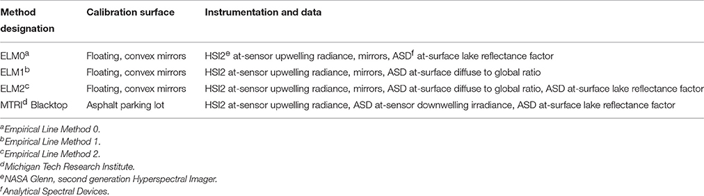
Table 1. Reflectance calibration methods employed.

In the empirical mirror calibration method designated ELM0, the Sun's downwelling irradiance hits the mirror surfaces and is radiated back up to the HSI2 senor flying above the target during an overpass. The ratio of the HSI2 radiance divided by the radiance reflected from the mirror is calculated to yield a biased estimate of the at-sensor reflectance factor. The measurement is biased due to the dispersion of light by the curved mirror surfaces. A gain factor for the mirror is then calculated by dividing the biased estimate of the at-sensor reflectance factor with the 100% Spectralon™-calibrated, at-surface reflectance factor measurement obtained from an ASD FieldSpec^® HH2 spectroradiometer to remove the bias. This single-point gain factor is then used to correct the mirror signal to determine a reflectance factor from the HSI2 radiance. This correction depends on knowledge of the observed at-surface reflectance of the target, measured using an ASD FieldSpec^® HH2 spectroradiometer. For the single-point empirical mirror calibration method (ELM1), we use a combination of the mirror radiance and the diffuse to global ratio measured using an upward looking ASD FieldSpec^® HH2 spectroradiometer equipped with a cosine-theta receptor to determine the mirror gain function. For the two-point empirical mirror calibration method, we add the use of the ASD at-surface lake reflectance factor, which yields the intercept for the reflectance factor in addition to the gain of the relationship. Derivations and equations for the ELM0, ELM1, and ELM2 methods based on radiative transfer theory are described below.

The MTRI blacktop calibration method does not employ mirrors to remove the atmospheric effects. Rather, that method starts with an at-sensor reflectance factor ratio determined by dividing the HSI2 radiance using the at-sensor irradiance measured by the upward looking ASD FieldSpec^® HH2 equipped with a cosine theta receptor that is mounted in the aircraft. A gain function is then determined by comparing the at-sensor reflectance factor to the well-known measurement of the reflectance factor of the asphalt blacktop parking lot at MBSP, which is measured routinely by researchers throughout the summer. The cosine theta irradiance data is adjusted to the same time of day as the parking lot reflectance factor data to minimize sun angle offsets.

Because each of these methods employs data from multiple instruments, it is possible that minor path radiance biases may be introduced by the fact that not all measurements are coincident in time or space. The ELM0 method should exhibit minimal path radiance bias because the reflectance factor ratio that removes atmospheric effects is determined using the same instrument, the HSI2. Any offset with this method arises from the calculation of the gain function by comparison with the surface reflectance factor measurement. This effect should be minimal, however, as the surface reflectance factor should vary more slowly than atmospheric measurements. The ELM2 method should yield a better estimate of the absolute reflectance factor than the ELM1 method, since it provides a more complete correction that accounts for both the slope and intercept. Offsets in the MTRI blacktop method could arise from calculation of the at-sensor reflectance factor using three separate instruments, or from the temporal and spatial offset of the path radiance between the measurements over the lake and the calibration data obtained from a nearby ground station.

We used the Kent State University (KSU) Varimax-rotated Principle Component Analysis (VPCA) visible derivative spectral decomposition method to partition the variance of the reflectance factor from the resulting derivative-transformed reflectance images. The resulting VPCA spatial score maps were smoothed with a 9 × 9 median kernel for presentation. The VPCA method allows us to compare the level of path radiance bias observed in the four, empirical reflectance factor calibration methods. This is a stringent test because the VPCA method is based on the derivative of the spectra and is capable of separating correlated signal from systematic bias and random noise (Ali et al., 2013; Ortiz et al., 2013). The KSU VPCA approach should thus be effective at separating path radiance biases resulting from scattering of light on the blue end of the spectrum from the spatially coherent, environmental signals. We predict that the ELM1 and ELM2 methods will yield similar VPCA signals since they differ only by a constant. Because the derivative of a constant is zero, the addition of the second calibration point, while necessary to yield accurate absolute reflectance factor values, should contribute little to the derivative spectra. In the sections that follow, we present theoretical derivations and empirical descriptions of the methods employed to convert from radiance to reflectance and to decompose the complex, mixed signals into independent spectral signatures that can be related to know color producing agents.

Deriving the Effective Lambertian Reflectance Factor of a Spherical Mirror

The empirical calibration of aerial and satellite systems to retrieve surface reflectance factor requires that the reference target have a known Lambertian reflectance factor. To use a ground reference target made of spherical convex mirrors, the specular reflectance factor of the mirror target must be converted to a Lambertian reflectance factor producing an equivalent sensor response in each spectral channel for the view angle recorded in the sensor image. The derivation of the transformation used in this analysis is described in this section. The spherical convex mirrors deployed on the water surface are domes designed to reflect a fraction f of the hemispherical sky toward the sensor as given by

where θ_m is the angular width of the mirror surface as measured from the mirror's center of curvature. A virtual image of the full hemispherical sky (f = 1) is seen in the mirror by a nadir looking sensor when θ_m = 45°. Schiller and Silny (2010) have shown that when illuminated by a hemispherical irradiance on a horizontal surface from the sun and the sky (${E_{sun}^{surf}(\lambda )+E}_{sky}^{surf}(\lambda )$; Watts m⁻² nm), that the upwelling radiance ($L_m^{surf}$; Watts m⁻² sr⁻¹ nm⁻¹) from a panel of N convex mirrors can be calculated knowing the radius of curvature of the mirrors (R_c) and the along-scan and cross-scan ground sample distance (GSD) of the sensor system (GSD_AS and GSD_CS, respectively) using the equation:

where ρ_m(λ) is the specular reflectance of the mirror measured in the laboratory. It is important to note that by using spherical mirrors, there is no foreshortening effect as with a flat diffuse target. Thus, the upwelling radiance signal is constant and independent of the sensor view angle and in principle, the tilt of the sphere representing the mirror's surface. Although the wave motion changes the orientation of the hemisphere reflected by a mirror so that the 180° Field of view may include some of the water surface if f = 1, the effect can be minimized by designing the mirrors to reflect a sky fraction slightly <1, if one assumes the integrated diffuse sky is relatively isotropic. As long as the direct solar contribution continues to be reflected at the sensor, a constant upwelling radiance will be maintained even for off-nadir view geometries of <25°.

Next, we establish a hemispherical-directional reflectance factor distribution function, ${\rho }_m^{HDRF}$, for the mirror reflectance factor target by taking the ratio of the radiance directed toward the sensor to the horizontal irradiance at the surface (Schaepman-Strub et al., 2006). Since there are no significant directional effects in the upwelling signal, applying Equation (2), one can write:

Here, we have included the term $\left[\frac{1}{\cos {\theta }_o}+\left(f-\frac{1}{\cos {\theta }_o}\right)G(\lambda )\right]$, which includes the solar zenith angle, θ_o, and the diffuse-to-global ratio illuminating a horizontal surface [G(λ)]. This term is needed to perform a proper conversion of specular reflectance to an equivalent Lambertian reflectance factor. It corrects for the fact that there is no foreshortening in the solar contribution to the mirror reflected signal compared to a Lambertian surface. A more detailed description of this correction term will be presented in a future publication.

Finally, Palmer (1999) shows that a reflectance factor distribution function, such as ${\rho }_m^{HDRF}$, is related to a hemispherical-to-direct Lambertian reflectance factor, ${\rho }_m^{HDRF}$, through a simple factor of π steradians. Thus,

The result is that Equation (4) provides the needed transformation equation for converting the specular reflectance spectrum of the mirror reference target to an equivalent Lambertian reflectance factor needed for the empirical calibration of the sensor image radiance to surface reflectance factor.

Empirical Line Method Reflectance Factor Calibration

The ELM applied to a lake surface image assumes a linear relationship between at-sensor water radiance, $L_w^{sen}\left(\lambda \right),$ recorded by the HSI2 imaging system and water surface reflectance factor, ${\rho }_w^{HDRF}\left(\lambda \right)$. This can be expressed for a sensor image calibrated to radiance as:

In terms of a linear equation, g_m(λ) is the gain function that will be derived from the mirror surface reference target and g_m(λ)(L_p(λ) + d(λ)) = b(λ) is the linear intercept. The term L_p(λ) is the atmospheric path radiance between the aircraft and the surface, while d(λ) accounts for any residual sensor calibration dark bias drift and potential processing offset. The empirical line equation follows as:

The determination of the gain and bias coefficients is obtained by regressing observed radiance values, recorded by the HSI2 sensor, against known reflectance factor values in each band from at least a high and low reflectance factor target pair in the scene. For the ELM1 solution, the coefficients needed to determine the intercept, b(λ) are set to zero, while both the slope and intercept coefficients are used for the ELM2 solution. This allows us to determine the impact that both the slope and intercept have on the solution. The high reflectance factor reference is provided by the convex mirror target deployed on the water and the low reflectance factor reference is recorded by a direct measurement of the water surface reflectance factor from a research vessel in the scene, or measurement from a nearby ground station. Thus, the calibration is based on the two reference points ($L_m^{sen}\left(\lambda \right),{\rho }_m^{HDRF})$ and ($L_{w,boat}^{sen}\left(\lambda \right),{\rho }_{w,boat}^{HDRF}),$ where $L_m^{sen}(\lambda )$ and $L_{w,boat}^{sen}(\lambda )$ are the HSI2 measured reference radiance of the mirror target and water surface and ${\rho }_{w,boat}^{HDRF}$ is the reflectance factor recorded at the location of the research vessel, or nearby ground station.

Thus, for the ELM2 solution, the image calibration equation converting all pixels in the scene from at-sensor radiance, $L_w^{sen}(\lambda )$, to at-surface reflectance factor, ${\rho }_w^{surf}(\lambda ),$becomes:

and provides an algorithm for performing an atmospheric correction of hyperspectral or multispectral image data. The ratio $\frac{{\rho }_m^{HDRF}(\lambda )}{L_m^{sen}(\lambda )}$ represents the mirror gain function g_m(λ).

One advantage obtained by the use of curved mirrors is that their convex shape disperses the light reflected back to the air- or space-bourne sensor passing over the target. This decreases the possibility that the solar radiance reflected from the surface will saturate the detector. The dispersion factor is determined as part of the calibration process. The approach effectively converts a passive spectroradiometer to an active spectrophotometer by sacrificing a small number of scene pixels. An additional advantage of the mirror targets for deployment is that they are small and generally can be designed to be the size of an instantaneous field of view (IFOV) pixel or smaller. As a result, the deployment of reflectance factor reference targets on water now becomes practical. If actual Lambertian-like targets were placed on the water instead of the mirror targets, their surface area would need to be at least 25 times larger in order to provide a reliable measure of the target radiance. This is due to the blurring resulting from the aircraft motion, the optical point spread function (PSF) and pixel resampling, all of which have the effect of mixing the reference signal with the background. The blurring effects can be seen in (Figure 2A), which shows the image of the mirror target deployed on the water surface. Although the target (1.2 m on a side) is smaller than the processed image pixels (3.21 m on a side), the radiance signal recorded by the sensor has been spread out over many pixels around it. Thus, the radiance from the target pixels is a combination of the mirror signal and the background water. However, because the target is small, it can be assumed to be a point source, located on a uniform background. It is thus straightforward to separate the total target radiance from the background water. An integration to remove the background is carried out by placing an integration window containing P pixels around the target centroid enclosing all the radiance from the target (Figure 2A, red box), as defined by the system PSF, and calculating the average radiance spectrum, $\overline{L_m^{sen}}(\lambda )$. Outside the perimeter of this window, an average pixel water radiance spectrum is derived, $\overline{L_w^{bkg}}(\lambda )$, to represent the background signal (Figure 2A, green box). Thus, the calculation of the background subtracted at-sensor total integrated radiance from the mirror target becomes:

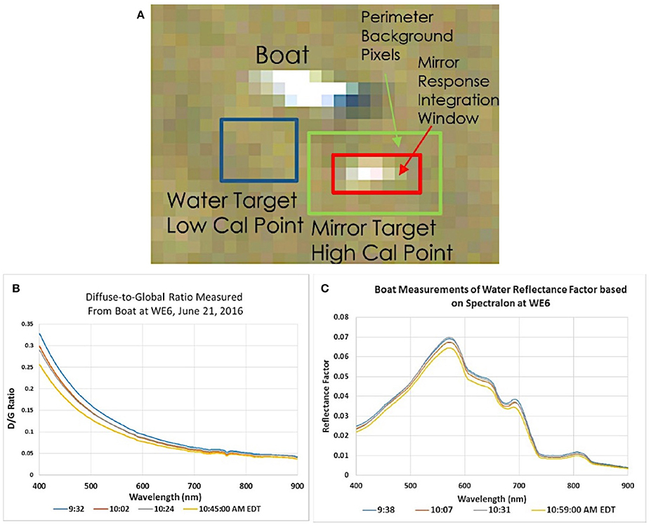
Figure 2. (A) NASA Glenn, second generation Hyperspectral imager (HSI2) image pixels from swath 15_MBSP, acquired on June 21, 2016, of the mirror reflectance target (red box: high calibration point), water (blue box: low calibration point) and boat at station Western Erie 6 WE6. Though the mirror target is smaller than an instantaneous field of view (IFOV) pixel, the energy reflected at the mirror is spread out over multiple pixels due to the aircraft motion, sensor system point spread function and pixel resampling during processing. Pixels included in target integration are indicated by green and red boxes. (B) Example diffuse to global ratio spectra, and (C) water surface reflectance spectra measurements taken from the boat located at WE6 on June 21, 2016.

Equation (8) provides the at-sensor radiance response for completing the calculation of the mirror gain function.

To fully explore parameter space, we also consider a different single-point calibration, the ELM0 method, which is based on the at-surface water reflectance factor, ${\rho }_{w,boat}^{HDRF}$, measured with an ASD FieldSpec^® HH2 at the boat location, rather than the mirror target reflectance factor ${\rho }_m^{HDRF}(\lambda ).$ This method first uses the mirror signal to remove the atmosphere by determining a ratio of the water leaving radiance and mirror radiance with both quantities measured directly by the HSI2 sensor. Because that ratio is biased by the mirror dispersion, it is rescaled using the at-surface reflectance factor measured from the boat with an ASD FieldSpec^® HH2 spectroradiometer. After algebraic re-arrangement, the mirror terms drop out and the radiance to reflectance conversion equation for the ELM0 has the form:

While this transformation will not yield absolute reflectance, it should be scaled so that spectra at various spatial locations in the scene have the correct spectral shape as needed for algorithms based on spectral shape, such as the KSU VPCA spectral decomposition method. We compare the results of the ELM0, ELM1, and ELM2 solutions with the MTRI Blacktop calibration, which is described below.

Results

Application of the Mirror-Based Empirical Line Method

The steps in the analysis of the data include the following for each HSI2 swath. We obtain the subset of the swaths that includes locations of ground-based measurements conducted by researchers in a vessel on the water or at a nearby ground station. We then identify the location of the research vessel and floating mirror array in the swath (Figures 1, 2A). The pixels associated with the mirror array (Figure 2A) are extracted and averaged, as are lake pixels near the mirror array. The image cutout of the mirror target and boat are shown in (Figure 2A) identifying the target integration window and pixel locations used to estimate the water background. The mirror correction method for the ELM1 and ELM2 is then applied using Equation (7) as described in the text and for the ELM0 using Equation (9). Validation data collected on the lake included measurements of the diffuse to global ratio obtained from the ratio of shaded to unshaded downwelling solar irradiance measured with an upward looking ASD FieldSpec^® HH2 spectroradiometer equipped with a cosine theta receptor (Figure 2B) and measurements of the at-surface reflectance factor relative to a 100% Spectralon™ plate measured with a downward looking ASD FieldSpec^® HH2 spectroradiometer equipped with a 10° FOV foreoptic (Figure 2C). The data in Figures 2B,C document the stability of the atmosphere and lake surface during data collection.

With knowledge of the sensor GSD for the image, the calculation of the mirror Lambertian reflectance factor, ${\rho }_m^{HDRF},$ can be completed. The specular reflectance spectra of the mirrors were measured at Kent State University using a Konica Minolta CM-2600d Spectrophotometer, which was set to measure the specular component of the reflectance factor relative to daylight with a brightness temperature of 6,500K. The calibration panel consisted of N = 16 mirrors deployed on the water surface. The radius of curvature for the mirrors, R_c = 20.1 cm, and a hemispherical sky fraction was calculated as f = 0.878. The resulting specular reflectance factor and Lambertian equivalent reflectance factor spectra, calculated from Equation (4), are shown in Figure 3A. The reference target is spectrally flat, which is ideal for the calibration of a hyperspectral sensor. Note that a calibrated, diffuse reflectance factor flat panel delivering a reflectance factor of 18% as shown in Figure 3A would normally saturate a sensor designed to record a high SNR for water leaving radiances. However, since the energy from the curved mirrors is spread over many pixels by the sensor PSF, a small bright target can be recorded without saturation, providing a measurement of the target signal with good precision. Figure 3B shows both the resulting average HSI2 water radiance spectrum representing the low calibration reference spectrum, $L_{w,boat}^{sen}(\lambda ),$ denoted with the blue box in Figure 2A and the net integrated HSI2 target radiance with background subtraction as calculated using Equation (8), $L_m^{sen}(\lambda ),$representing the high calibration radiance spectrum. The ratio of the at-surface mirror target reflectance factor spectrum and HSI2 measured at-sensor mirror target integrated radiance spectrum provides the mirror gain function used to convert any HSI2 radiance spectrum to surface reflectance factor in the scene via Equation (7), assuming even illumination throughout the scene.

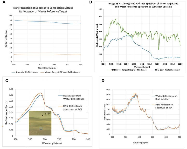
Figure 3. (A) Specular reflectance factor and Lambertian equivalent reflectance factor spectra, calculated from Equation (4). (B) Resultant average NASA Glenn, second generation Hyperspectral imager (HSI2) water and mirror radiance spectra representing the low calibration reference spectrum (HSI2 Boat Water Spectrum) and the high cal reference (HSI2 Mirror Target Integrated Radiance). (C) Empirical line method 2 (ELM2) transformation reflectance spectra of water pixels extracted from the HSI2 15_MBSP swath (inset, red region of interest; ROI), compared to in situ reflectance spectra measured concurrently using the Analytical Spectral Devices (ASD) FieldSpec HandHeld 2 (HH2) around the boat at station WE6 (insert, blue box). (D) Empirical line method 0 (ELM0) transformation reflectance spectra of the same pixels shown in (C) for comparison.

The at-sensor radiance to surface reflectance factor transformation is demonstrated in Figure 3C as the average water radiance spectra, based on HSI2 pixels around the boat and mirror targets that were extracted from a portion of the 062116_15_MBSP swath, which is shown in the inset image in Figure 3C. Applying Equation (7) as a two-point calibration (ELM2), the transformation to a predicted at-surface reflectance factor spectrum was calculated and shown in the plot for two locations, the boat location in the blue box and a second, independent region of interest (ROI) in the red box. The result produces an estimated absolute reflectance factor water surface spectrum at each location. The predicted spectrum at the boat is identical to the ASD measured reflectance factor spectrum at the research vessel (10:31 a.m. EDT Figure 2C) because it was recorded nearly coincident with the HSI2 overpass (3 min apart) and was used as the low reference reflectance spectrum for calibration and thus sits exactly on the line defined by Equation (7). The second spectrum in red is the resulting reflectance factor spectrum for an independent ROI location. The two spectra represent the absolute appearance of the water reflectance factor spectra at the two locations recorded by the HSI2 sensor as scaled in reflectance units by the mirror gain function. The two-point calibration transformation removes the solar/sky illumination spectrum and the atmospheric transmittance and path radiance effects produced between the sensor and the water surface extracting the water reflectance factor spectrum for the illumination and view geometries at the time of the HSI2 collect. In comparison, Figure 3D shows the resulting transformation using only the mirror gain function in a single-point calibration (ELM1) without the bias correction provided by the ASD measured at-surface water reflectance [the terms for ${\rho }_{w,boat}^{HDRF}$ and $L_{w,boat}^{sen}(\lambda )$ were set to 0 in Equation (7)]. The resulting spectrum has similar shape, but more noise than the EML2 spectrum from Figure 3C, and a higher path radiance contribution on the blue end of the spectrum. The ELM1 calculation will allow us to determine if the KSU VPCA spectral decomposition analysis can still be performed in this way using less ground validation data. The mirror gain function correctly scales the relative difference between the two locations in reflectance units for the ELM2, but a spatially constant reflectance offset in each spectral band still remains as revealed in the difference between the spectra in Figures 3C,D. Though the result is not an absolute reflectance spectrum, the ELM1 spectrum can still potentially be used for spatial/spectral decomposition. This will be explored in Section Comparison of the Reflectance factor calibration methods: VPCA Decomposition.

The important result is that the methodology of deploying a single mirror reflectance factor reference target was successful in performing an atmospheric correction of the HSI2 aircraft imagery resulting in the retrieval of the at-surface water reflectance factor spectral profiles based on the image data, sensor metadata, the mirror target properties, measurements of the lake surface reflectance and simple measurements of shaded and unshaded downwelling solar irradiance to establish the diffuse to global ratio. The utility of the derived spectra will be demonstrated in the following sections, where we compare the ELM0, ELM1, and ELM2 reflectance factor estimates with the extraction of water constituents using the KSU VPCA spectra decomposition method. Though random path radiance bias is likely present between the derived HSI2 and the surface validation spectrum due to offsets in time of measurement and/or location, they will mostly drop out in the derivative transformation and decomposition process with minimal effect on the analysis results.

MTRI Blacktop Calibration Results

We compare the three mirror-based reflectance calibration methods with an additional empirical approach to estimate the reflectance factor. The MTRI blacktop vicarious calibration method involves identifying a natural or artificial site that can be measured both by the HSI2 sensor, which requires calibration, and instruments of known calibration, such as the ASD FieldSpec^® HH2 spectroradiometers used in our field measurements. The ratio of these measurements is used as the basis for the vicarious calibration. The MBSP parking lot was chosen as a suitable location because the site is located along the immediate shoreline of Lake Erie so that it does not impose an undue burden on flight planning and navigation; the parking lot has a consistent and well-characterized spectral response across both time and space (Figure 4A); and is a relatively large feature that can be easily identified in HSI2 imagery at any operational elevation (Figure 4B).

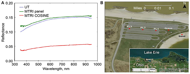
Figure 4. (A) Maumee Bay State Park (MBSP) parking lot blacktop spectral response, as measured by MTRI and the University of Toledo (UT) research teams. (B) NASA Glenn, second generation Hyperspectral imager (HSI2) image of MBSP parking lot in relation to Lake Erie (insert) (After Figures 4.2 and 4.3, Lekki et al., 2017).

The correction factor (Figure 5), which is a wavelength-dependent scalar that relates the two reflectance factor measurements, is then calculated using Equation (10), where C is a correction coefficient, λ is wavelength, Cal_Ref is the calibrated reflectance factor (i.e., ASD radiance/ASD irradiance measured in situ at MBSP), and Uncal_Ref is the uncalibrated reflectance factor (i.e., HSI2 radiance/ASD irradiance upward looking from the S3 Viking aircraft). The correction factor equation will encapsulate the measurement differences between the two sensors, including all sources of measurement error, and can be used to convert measurements from one instrument into the other. Of obvious interest is converting the uncertain sensor to match the well-calibrated instrument.

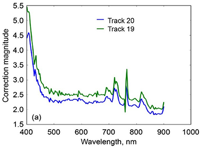
Figure 5. Wavelength-specific correction coefficients derived from comparing to in situ reflectance for two NASA Glenn, second generation Hyperspectral imager (HSI2) tracks (track 19 and 20) (After Figures 4.5, Lekki et al., 2017).

Radiance and irradiance spectroradiometer measurements were recorded to calculate an at-sensor surface reflectance factor. Coincident ground data was collected during overflight using ASD FieldSpec^® HH2 spectroradiometers set up in the MBSP parking lot. This allows collection of data under the same illumination conditions as the lake surface from a nearby ground station. We account for the effects of solar angle on the diffuse illumination component of radiance when a cosine receptor is used to measure irradiance by applying a time correction. When using a 100% Spectralon™ panel, mirror, or other known reflector to estimate solar radiance, the effect of the diffuse terms will cancel out when computing the reflectance factor. The cosine receptor does not include this term, whereas the radiance measurement does, and will therefore remain in the computed reflectance factor if not addressed. An example of this effect is readily apparent (Figure 6A) in the split between the 10:30 and 13:00 measurements from the MTRI ASD FieldSpec^® HH2 data collected on August 24, 2015, in which the time correction for solar angle removes most of the offset (Figure 6B).

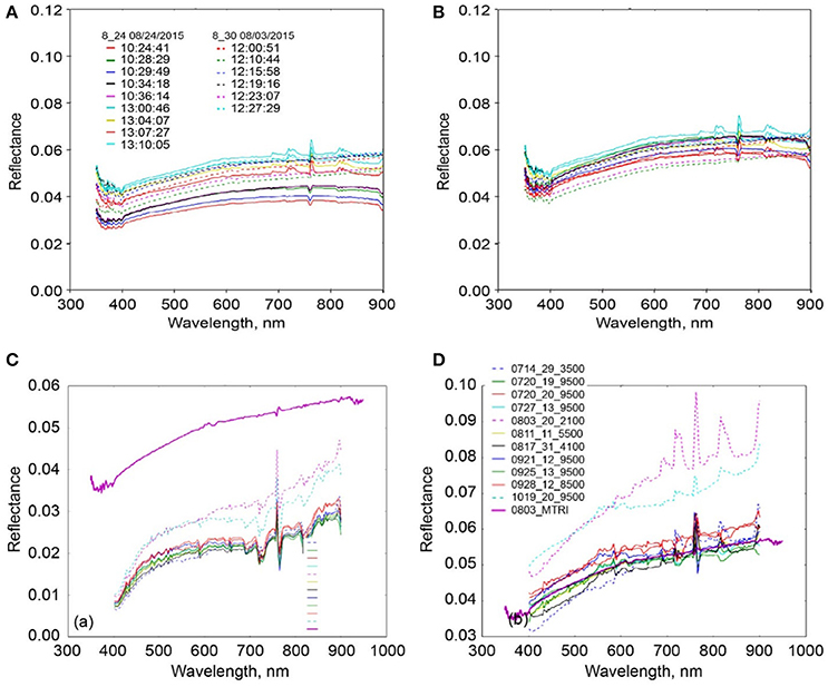
Figure 6. (A) Maumee Bay State Park (MBSP) in situ reflectance before time correction. (B) MBSP in situ reflectance after time correction. (C) NASA Glenn, second generation Hyperspectral imager (HSI2) parking lot reflectance uncorrected. (D) NASA HSI2 parking lot reflectance corrected. In situ reflectance is shown in magenta (labeled 0803_MTRI) in (C,D) (After Figures 4.4 and 4.6, Lekki et al., 2017).

We explore output from the MTRI method using data from a number of swaths collected in 2015. In Figure 6C, the parking lot as observed by the HSI2 sensor has a similar shape in spectra extracted from different swaths; the remaining differences are likely atmospheric or time of day effects. This suggests that a single correction factor would be useful even on days for which it was not recomputed, as demonstrated by the manner in which the corrected signals clustering around the observed ASD FieldSpec^® HH2 spectra (Figure 6D). The two anomalous dates are both flagged as cloudy days (dashed line), their measurement difference could be explained by clouds periodically shadowing the irradiance measurements, which were averaged across the entire track, leading to a higher than normal reflectance factor measurement. The measurements thus likely differ due to variations in the diffuse to global ratio for cloudy vs. clear sky.

Reflectance Factor Inter-Comparison

To explore the hyperspectral nature of the reflectance factor signals, we compare the average reflectance spectra from each reflectance factor calculation and their derivatives (Figure 7). To more clearly compare the spectral shapes for each reflectance factor calculation, we convert the averages to z-scores, by subtracting the average reflectance value across all wavelengths in the visible and dividing by the standard deviation across all wavelengths in the visible. These standardized reflectance values and standardized derivatives are a useful way to compare the results because the VPCA method is based on analysis of the correlation matrix of the derivative spectra. The four methods of calculating the reflectance factor produce values that range in amplitude from minimum to maximum reflectance by 1.8 to 14.8%. None of the average spectra exhibited negative reflectance factors. The ELM0 method produced the lowest amplitude signal, while the ELM1 method produced the largest amplitude signal. The ELM1 and MTRI exhibited higher reflectance factors on the blue end of the spectrum relative to the ELM0 and ELM2 methods. This is particularly apparent when viewing the z-score transformed reflectance factors (Figure 7B). When the results were z-score transformed, the similarity in spectral shape of the four methods of calculating the reflectance factor is readily apparent as is the increased blue-end reflectance for the ELM1 and MTRI methods relative to the ELM0 and ELM2 methods. The derivative spectra for both the absolute reflectance factor values and the z-score transformed observations were similar, exhibiting the same spectral features, although they diverged to some extent toward the blue end of the spectrum.

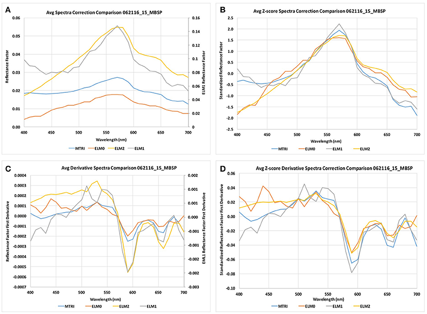
Figure 7. (A) Comparison of average scene spectra for each correction method. (B) Comparison of z-score correction of average scene spectra. (C) Comparison of average derivative scene spectra for each correction method. (D) Comparison of z-score correction of average derivative scene spectra for each correction method.

The ELM2 provides the best estimate of the absolute reflectance as demonstrated by the goodness of fit with the measured at-surface ASD FieldSpec^® HH2 surface reflectance factor. The MTRI and ELM0 methods produced reflectance spectra of similar amplitude, while the ELM2 values had higher amplitude. The ELM1 values were considerably higher than the ELM2 estimates because the intercept term in Equation (8) for the ELM1 calculation was intentionally set to zero to explore the impact of the intercept on the solution. In terms of absolute reflectance, there is a bias offset for the ELM0 and MTRI relative to the absolute spectrum produced by the ELM2 transformation, but less offset than for the ELM1 transformation. As predicted, the ELM0 and ELM2 solutions have the same spectral shape as can be seen for the z-score transformed results (Figure 7B). We further explore the differences between the ELM0, ELM1, ELM2, and MTRI calculations in the following section where we evaluate the underlying structure of the images using an eigenvalue-eigenvector decomposition method, the KSU VPCA spectral decomposition method.

Comparison of the Reflectance Factor Calibration Methods: VPCA Decomposition

The four reflectance factor calculation methods listed in Table 1 when applied to HSI2 swath 062116_15_MBSP produce reflectance RGB plots that look very similar (not shown) to the radiance RGB plot in Figure 8A. The dominant pattern observed in the radiance RGB image for the swath are alternating bands and filaments that run parallel to the coast, which is located at the bottom of the image. There is a strong coastal transition front that marks the end of the reddish-brown coastal waters and the transition into the bluish-green offshore waters of the Western Basin. The coastal water appears more red than the offshore waters, located further into the Western Basin. A second, strong brighter-colored front can be seen toward the top of the swath. This front separates milky blue water to the south in the middle of the image that transition into water of more buff coloration to the north, before transitioning furthest offshore into a darker, blue color. Because of the similarity of the reflectance-derived RGB images, the MTRI reflectance method was used to calculate the Cyanobacterial Index (CI) (Wynne et al., 2010, 2013). The calculation of the widely-used NOAA CI, contributed by collaborators at UT, provides a useful reference for comparison to the components extracted using the VPCA decomposition method. For comparison with VPCA score maps, the spatial map of the NOAA CI was smoothed with a 9 × 9 median kernel for presentation as was done with the VPCA score maps.

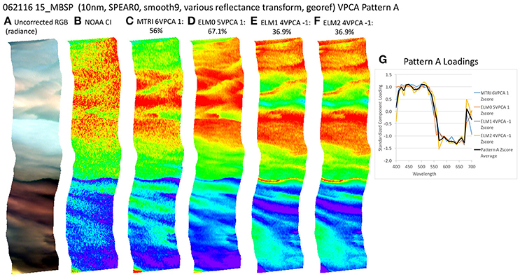
Figure 8. (A) Red, Green, Blue (RGB) image of swath 15_MBSP from June 21, 2016. (B) National Oceanic and Aeronautical Administration Cyanobacterial Index (NOAA CI) product calculated after Wynne et al. (2010). (C) Spatial distribution of varimax-rotated principal component analysis (VPCA) component pattern A using Michigan Tech Research Institute (MTRI) correction method decomposition. (D) Spatial distribution of VPCA component pattern A using Empirical Line Method 0 (ELM0) correction method decomposition. (E) Spatial distribution of VPCA component pattern A using Empirical Line Method 1 (ELM1) correction method decomposition. (F) Spatial distribution of VPCA component pattern A Using Empirical Line Method 2 (ELM2) correction method decomposition. (G) Pattern A Loadings. Negative signs in loading numbers indicate that pattern has been multiplied by −1 for comparison purposes.

Application of the KSU VPCA spectral decomposition method following (Ortiz et al., 2013; Lekki et al., 2017) to the four reflectance factor data sets enabled extraction of four to six components that account for a maximum of 92.8–97.4% variance in the four derivative transformed data sets (Table 2). One difference among the various solutions is that in some cases, the components extracted were flipped relative to similar components from one of the other calculation methods. This is a function of the varimax rotation. It can be easily addressed by multiplying the component scores and loadings by −1, so that the components with similar shape and spatial pattern have the same sign. This has been done for ease of comparison between components. The ELM0 solution explained the largest amount of variance in the image at 97.4% for five components (Table 2). The components extracted from the other reflectance factor methods exhibit subtle differences from each other, but their general similarity is readily apparent (Figures 8–13).

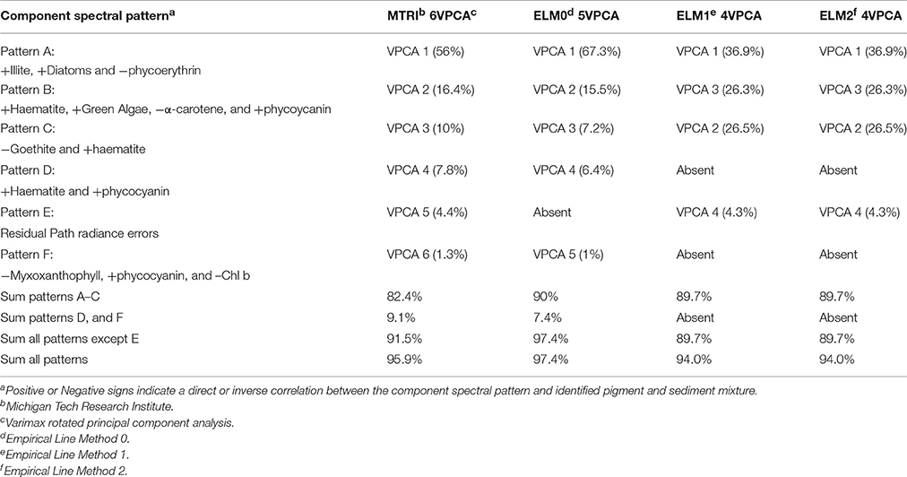
Table 2. Correlation of spectral patterns and variance explained.

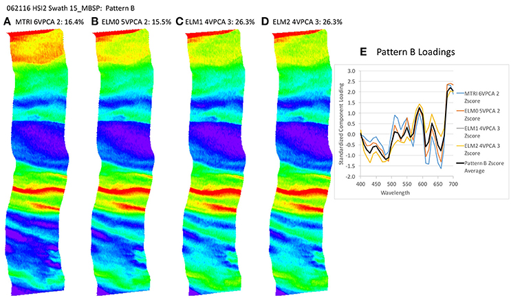
Figure 9. Spatial distribution of varimax-rotated principal component analysis (VPCA) component pattern B. (A) Michigan Tech Research Institute (MTRI) correction method decomposition. (B) Empirical Line Method 0 (ELM0) correction method decomposition. (C) Empirical Line Method 1 (ELM1) correction method decomposition. (D) Empirical Line Method 2 (ELM2) correction method decomposition. (E) Pattern B Loadings.

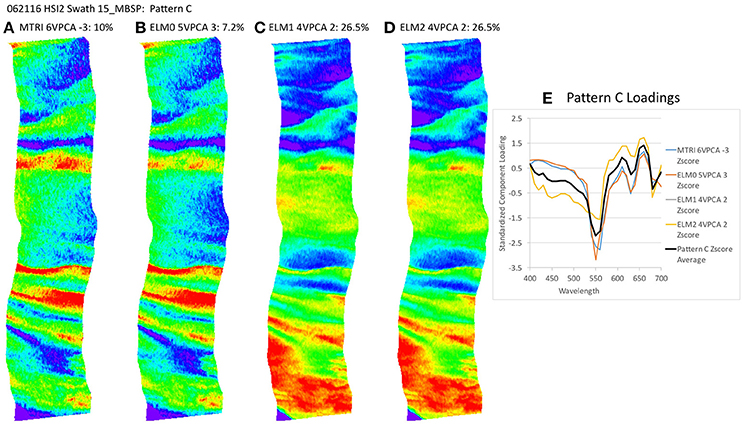
Figure 10. Spatial distribution of varimax-rotated principal component analysis (VPCA) component pattern C. (A) Michigan Tech Research Institute (MTRI) correction method decomposition. (B) Empirical Line Method 0 (ELM0) correction method decomposition. (C) Empirical Line Method 1 (ELM1) correction method decomposition. (D) Empirical Line Method 2 (ELM2) correction method decomposition. (E) Pattern C Loadings. Negative signs in loading numbers indicate that pattern has been multiplied by -1 for comparison purposes.

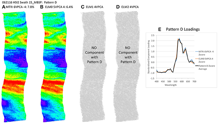
Figure 11. Spatial distribution of varimax-rotated principal component analysis (VPCA) component pattern D. (A) Michigan Tech Research Institute (MTRI) correction method decomposition. (B) Empirical Line Method 0 (ELM0) correction method decomposition. (C) Empirical Line Method 1 (ELM1) correction method decomposition. (D) Empirical Line Method 2 (ELM2) correction method decomposition. (E) Pattern D Loadings. Negative signs in loading numbers indicate that pattern has been multiplied by -1 for comparison purposes.

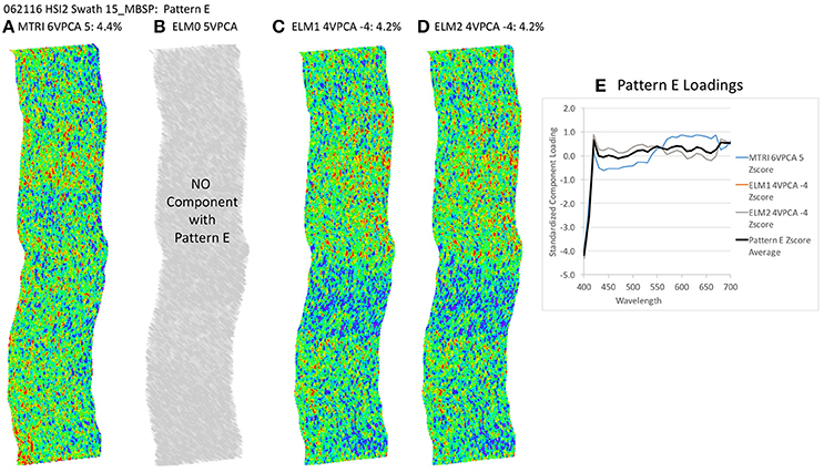
Figure 12. Spatial distribution of varimax-rotated principal component analysis (VPCA) component pattern E. (A) Michigan Tech Research Institute (MTRI) correction method decomposition. (B) Empirical Line Method 0 (ELM0) correction method decomposition. (C) Empirical Line Method 1 (ELM1) correction method decomposition. (D) Empirical Line Method 2 (ELM2) correction method decomposition. (E) Pattern E Loadings. Negative signs in loading numbers indicate that pattern has been multiplied by -1 for comparison purposes.

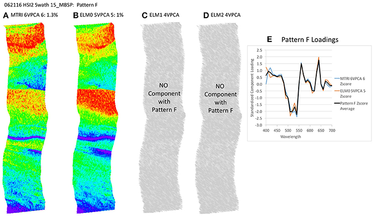
Figure 13. Spatial distribution of varimax-rotated principal component analysis (VPCA) component pattern F. (A) Michigan Tech Research Institute (MTRI) correction method decomposition. (B) Empirical Line Method 0 (ELM0) correction method decomposition. (C) Empirical Line Method 1 (ELM1) correction method decomposition. (D) Empirical Line Method 2 (ELM2) correction method decomposition. (E) Pattern F Loadings. Negative signs in loading numbers indicate that pattern has been multiplied by -1 for comparison purposes.

To identify the composition of the color producing agents in each component, we standardized the component scores, then matched the components from each data set without replacement to their best visual match (if any) in the other data sets to group them into spectral “patterns.” Comparing the various solutions, the components can be matched on the basis of their spectral shapes and spatial patterns into six patterns, labeled A through F (Table 2, Figure 14). The component loadings for the matches in the patterns were then averaged and compared using forward, least-squares, stepwise regression against a library of known standardized pigments and mineral spectra (Ortiz et al., 2013) to infer their composition. The quality of the identified patterns was determined by the spatial coherence of their component score maps, average spectral loadings < ±3 standard deviations, and absolute R-values for the stepwise regression >0.8.

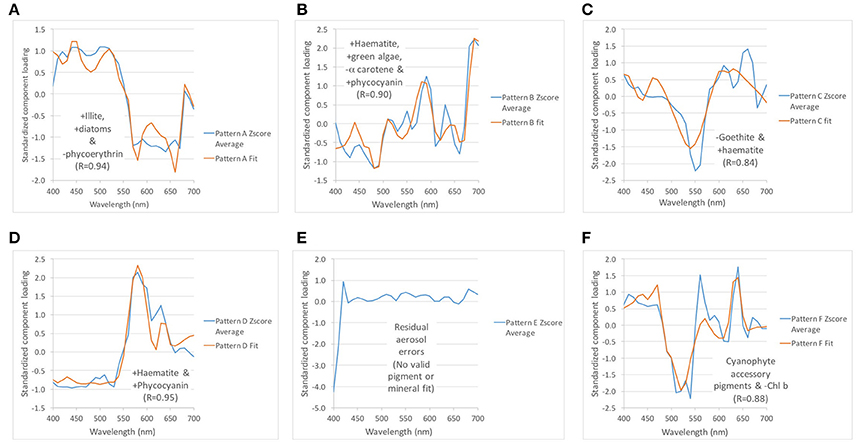
Figure 14. Spectral patterns of varimax-rotated principal component analysis (VPCA) components (A–F), indicating inferred composition based on forward, stepwise least squares regression. Complete description of the composition of each average component spectral pattern is listed in Table 2. The quality of the regression fit is indicated by the reported R-value.

The key point to address here is the similarity of the structure of the results extracted despite the differences in the atmospheric correction methods applied. All of these patterns (with the exception of Pattern E) exhibit coherent spatial structures, partitioning the variance in the hyperspectral image cube into graceful filaments and bands that run parallel to the coast. The NOAA CI and the VPCA solutions pull out features similar to those seen in the RGB images. The NOAA CI indicates bloom-like conditions offshore and then alternating bands of higher and lower values parallel to the coast, tapering out toward lower values near the shore. The leading component (Pattern A) extracted from the four data sets has a spatial pattern most similar to the NOAA CI (Figure 8B). The first three patterns are found in all four of the solutions and explain between 82.4 and 90% of the variance in the data sets (Table 2, Figures 8–10). Patterns D, F are each found in two of the four solutions (Figures 11, 13). They represent 6.4 or 7.8%, 1.0 or 1.3%, of the variance in each data set, respectively. The sum of all the coherent spatial patterns, which can be related to environment signals in the images accounted for 88.5–97.4% of the image variance.

These components can be partitioned into spatially coherent environmental signals and random noise. A detailed evaluation of the spectral interpretation of the components is beyond the scope of this paper and will be addressed in a separate paper, but Table 2 and Figure 14 identify the most likely composition of the spectral patterns based on stepwise multiple linear regression against known standards. Briefly, the components extracted from the image represent mixtures of sediment (illite, haematite, and goethite), and algal and cyanophyte groups and pigments known to be present in the waters of the western basin of Lake Erie (Ortiz et al., 2013). Matching the features present in the radiance-based true color image (Figure 8A), the reddish portions of the image were identified as containing iron-bearing minerals as well as autotrophs, while the offshore waters were identified as mixtures of lighter-colored illite, algae, cyanophytes, and various accessory pigments.

One notable difference between the ELM0 solution and the other three solutions is Pattern E, which is absent from the ELM0 solution, but present in each of the other three data sets (Figure 12). Pattern E exhibits a random spatial pattern and a spectral pattern with strongest loadings in the blue end of the spectrum. This pattern accounts for 4.3 to 4.4% of the variance in the data sets where it is found. The significance of Pattern E is discussed below. Expanding the MTRI decomposition to 6 components extracted a 6th component (Pattern F) that was similar to the 5th component in the ELM0 case. Expanding the ELM1 and ELM2 solutions out to a 5th or 6th component extracts a 5th component with a spectral pattern that cannot be matched to any know standards or mixtures in the spectral library in the 5-component case and splits the random noise component (Pattern E) in the 6th component case. This indicates that a 4-component solution is sufficient to capture all the variability in the ELM1 and ELM2 cases.

Discussion

Implications for Reflectance Estimation and Atmospheric Correction

A fundamental challenge associated with analysis of multispectral and hyperspectral visible remote sensing imagery is removal of atmospheric effects. Here we explore several different applications of empirical methods of atmospheric correction, which enables extraction and separation of mixed environmental signals from aquatic data sets. Development of atmospheric correction methods that are effective is important to enable optimal use of future, planned hyperspectral orbital missions, such as PACE, HyspIRI, and GeoCAPE. In this application, the question of interest is to identify the constituents present in the optically complex waters of the Western Basin of Lake Erie. This area develops a perennial CyanoHAB bloom that initiates in the late spring or early summer, depending on the level of runoff to the system (Stumpf et al., 2012; Bullerjahn et al., 2016). In general, the bloom is larger and starts earlier during wet years, and is smaller in dry years (Stumpf et al., 2012). The Maumee River and other rivers in the region deliver significant nutrient loads, suspended sediment and a variety of algal and cyanobacterial taxa into the Western basin (Conroy et al., 2014; Kane et al., 2014; Matisoff and Carson, 2014; Pennuto et al., 2014). As a result, the assumption that the optical properties of the water are controlled only by chlorophyll a is not valid (Ali et al., 2013, 2014; Ali and Ortiz, 2016). Removal of atmospheric effects enables further analysis of the reflectance spectra to determine which constituents are present at any given time. While several approaches have been proposed to do this, spectral shape-based algorithms show promise at partitioning the variance associated with these complex optical mixtures (Simis et al., 2005; Moisan et al., 2011; Chase et al., 2013; Shuchman et al., 2013). Application of these methods in these complex environments suggests that they will be effective at less complex marine applications. Indeed, a similar EOF analysis approach has been applied in the optically complex Baltic Sea (Soja-Woźniak et al., 2017) and the lead author, Ortiz, is applying the VPCA spectral decomposition method effectively using data sets collected in the USVI.

It is in this context that we compare the reflectance factor calculations. In our experience in the Western Basin, the ELM has proven to be very effective at removal of atmospheric effects, with modest amounts of input data (Lekki et al., 2017). We present a theoretical basis to support the ELM based on radiative transfer theory. To evaluate the effectiveness of the ELM method we employed two complementary means of removing the atmospheric effects: one approach used mirrors to directly measure the downwelling irradiance, while the MTRI approach calculates an at-sensor reflectance factor and then generates a gain function using the reflectance of a known surface to reshape the reflectance factor to at-surface values. The two methods are complimentary. The mirror based correction method is based on direct observation of the downwelling irradiance at one or more points in the scene and thus can be used as an effective check on other methods of atmospheric removal. The MTRI approach can be applied broadly in the absence of additional equipment that must be imaged in the scene (the mirrors), which are required to apply the mirror-based correction methods.

All four of the methods produced average reflectance factors that were positive, suggesting the in situ calibration data allowed the methods to yield reasonable reflectance factors. When plotted as a function of wavelength, the ELM0 method produced the lowest amplitude reflectance factor, followed by the MTRI, then the ELM2 and finally the ELM1 method, which is known to be biased, because it intentionally does not include an intercept correction (Figure 7). By presenting a theoretical explanation for a single-point and two-point ELM correction, we can illustrate the impact of path radiance on the resulting estimated reflectance factor calculations. The two-point ELM2 correction method outperforms the single-point EML1 correction method in terms of recovering absolute reflectance. The MTRI and ELM0 methods underestimated the maximum reflectance response relative to the two-point ELM method, but the ELM0 was able to capture the same spectral shape as the ELM2 method.

To compare the spectral shapes extracted by the four methods, the average reflectance factor for each method was standardized by removal of the spectral mean and then the residual was divided by the spectral standard deviation to calculate z-scores. Several important points arise from this comparison. First all of the values lie within 3 standard deviations, indicating that on average, the spectra did not include individual bands that were biased by extreme outliers. In addition, (Figure 7B) documents that all four methods have similar spectral shapes. The ELM0 and ELM2 spectral shapes are consistent throughout the visible. The MTRI and ELM1 spectra are also similar to each other. However, they both exhibit considerably more signal on the blue end of the spectrum than either the ELM0 and ELM2 spectra below ~475 nm. The MTRI and ELM1 spectra exhibit slightly less reflectance at wavelengths longer than 600 nm than either the ELM0 or ELM2 methods. Comparison of the derivative spectra for the four methods shows similar variability above 540 nm. The curves diverge somewhat toward the UV end of the spectrum. The similarity of the methods is particularly apparent in the derivative of the z-score spectra.

We can make some observations regarding what will happen if additional secondary analysis methods are applied to the reflectance factors to extract environmental information, such as chlorophyll a or other pigment concentrations related to the scene (e.g., Witter et al., 2009). Methods that rely on accurate absolute reflectance values will fail when applied to the ELM1 method, which was presented only to show the importance of the path radiance correction to a valid solution. Based on the strength of the theoretical basis presented, the ELM2 method will yield a stronger response than if either the MTRI or the ELM0 reflectance factor methods are employed. This may be less of an issue for band ratio based methods, particularly ones that operate toward the red end of the spectrum.

Spectral Shape and Identification of Component Patterns

The z-score analysis of the four methods shows that they each extract very similar spectral shapes. Methods that extract information about color producing agents based on a spectral shape will perform similarly with the four methods. To document this, we applied the KSU VPCA spectral decomposition method (Ortiz et al., 2013) to each of the four reflectance factor calculations presented here. The results presented in Figures 8–14 demonstrate this well. The leading component extracted in all cases is similar in spatial distribution to the NOAA CI. This is to be expected, because chlorophyll a is found in all taxa of algae and cyanobacteria and thus should dominate the signal. While the NOAA CI pattern look similar to the leading VPCA component for each case, the VPCA results are cleaner, because they are based on a centered, first derivative, rather than a second derivative as for the NOAA CI. Each higher order derivative calculation introduces more error when looking for small differences between large values (Press et al., 1992).

In addition, the VPCA method removes uncorrelated signal from the data set so that features that are not related to a particular pattern show up in other components, or are excluded as noise (Abdi, 2003). For this reason, the VPCA method is relatively insensitive to the noise that was left in the ELM1 solution by setting the intercept term to zero (Figure 3C vs. Figure 3D). Notice that the ELM1 and ELM2 spatial patterns for the VPCA solutions in Figures 8–13 are virtually identical because the two solutions differ only by a constant, which drops out during the derivative calculation step in the VPCA.

The VPCA spectral decomposition approach also provides additional information beyond that which the NOAA CI alone can extract. In this application, we were able to extract three to five consistent components with coherent spatial signals. This was true despite difference in the way that the atmospheric effects were removed or due to differences in the absolution reflectance factor estimates. This result strongly suggests that the KSU VPCA method, which is based on extraction of spectral shapes, is relatively insensitive to the need for absolute reflectance values. Atmospheric corrections that are adequate thus can yield valuable, higher-order information about the scene. The reason why this works is because the KSU VPCA spectral decomposition method is based on decomposition of the correlation matrix of the derivative spectra, rather than analysis of absolute reflectance factors. The derivative transformation removes scattering effects, while the correlation analysis decreases the need for stringently correct absolute reflectance factors. Obtaining a valid estimate of the spectral shape—the relationship between bands in the data set—is sufficient to yield useful results.

Correction for Imperfect Atmospheric Removal

Another problem that plagues conversion from radiance to reflectance is a lack of validation data that are precisely coincident with the overflight observations. In our case, the various methods presented require one or more of the following data for calibration or validation: downwelling irradiance, the diffuse to global ratio, and surface reflectance factor measurements of a known calibration surface on land or water for one or more different surface radiance values. Instruments that can simultaneously measure downwelling irradiance and upwelling radiance or reflectance are considerably more expensive than radiometric instruments that can only measure in one orientation at a time. Likewise, labs that maintain more than one instrument often opt to place them at multiple locations in the scene to assess spatial heterogeneity. The lack of strictly coincident data in space and time can thus lead to errors in calculations because the properties of the scene can shift with time as lighting or cloud cover changes.

The KSU VPCA spectral decomposition method provides a means of addressing and quantifying the impact of temporal variability in scene conditions on data acquisition. In our results, three of the four methods of calculating reflectance factors produced a random noise component, with the largest spectral response in the blue end of the spectrum and near zero responses at other wavelengths (Figures 12, 14E). This spectral and spatial pattern is consistent with path radiance effects that likely arise from ancillary data that are not precisely temporally or spatially coincident with the observations from the NASA Glenn HSI2. The only method that did not produce this path radiance component was the ELM0 method. Because the ELM0 method calculated a direct ratio of the downwelling and upwelling radiance measured over the full path length between the surface and the HSI2 sensor using data from that sensor only, this method did not produce a path radiance bias component during the VPCA spectral decomposition, even though its reflectance factor produced the lowest amplitude response. In addition to the temporal and spatial coherence of the measured downwelling and upwelling radiance ratio from the HSI2 used in the ELM0, this result also arises because the measured at-surface water reflectance factor spectrum used as the calibration point for the ELM0 transformation is closer in magnitude to the rest of the water surface across the scene than the higher mirror target reflectance factor used as the at-surface reflectance calibration point in the ELM1 and ELM2 transformation. Even so, the magnitude of the path radiance bias in the other methods was small, amounting to just 4.3–4.4% of the total variance extracted from the image. The ability of the KSU VPCA spectral decomposition method to partition this random bias from the environmental components extracted from the image further documents the usefulness of the method.

The work presented here documents that the empirical line method, used in conjunction with the KSU VPCA decomposition method is sufficiently robust to provide adequate atmospheric correction to hyperspectral visible image data. The use of derivative spectroscopy also provides a way to extract useful information even when the absolute reflectance values are not strictly correct as was demonstrated with the ELM1 test example where we specifically left off the intercept of the radiance to reflectance transformation. The VPCA method also explicitly removes path radiance issues that result from data that is not precisely temporally synchronous. These results are encouraging and indicate that as a field, we have methodologies in place that will enable the community to capitalize on the additional spectral information that can be extracted from proposed orbital hyperspectral sensors on missions such as PACE, HyspIRI, and GeoCAPE. Each of these sensors has been designed for specific missions. PACE will provide global hyperspectral coverage at daily temporal and 1 km spatial resolution. HyspIRI will provide high spatial resolution hyperspectral data (30 m) in the Landsat orbit to provide continuity with legacy Landsat data and the capability for highly enhanced data products. Finally, GeoCAPE is a proposed geostationary instrument that would image 70% of the illuminated western hemisphere, enabling the collection of time series of hyperspectral data for unprecedented process studies. Deploying these tools will create the opportunity for enhanced determination of pigment-related biomass estimates and new capabilities to identify algal and cyanobacterial composition based on extraction of pigment spectra by visible derivative spectroscopy as well as a host of other applications.

Conclusions

Our results document the utility of empirical calibration methods, such as the ELM to remove atmospheric errors from hyperspectral remote sensing data sets. We present a theoretical basis for the ELM using radiative transfer theory. The ELM2 and ELM0 methods produced spectral shapes that were consistent across the entire visible spectrum, but the ELM2 was effective at reconstructing the absolute reflectance values. The work presented here documents that the empirical line method, used in conjunction with the KSU VPCA decomposition method is sufficiently robust to provide adequate atmospheric correction to hyperspectral visible image data. The VPCA method extracted more information from the image swaths than the NOAA CI method, with less random error. The use of derivative spectroscopy also provides a way to extract useful information even when the absolute reflectance values are not strictly correct as was demonstrated with the ELM1 test example where we specifically left off the intercept of the radiance to reflectance transformation. In our results, three of the four methods of calculating reflectance factors produced a random noise component, with the largest spectral response in the blue end of the spectrum and near zero responses at other wavelengths. This spectral and spatial pattern is consistent with path radiance effects that likely arise from ancillary calibration data that are not precisely temporally or spatially coincident with the observations from the NASA Glenn HSI2. The only method that did not produce this path radiance component was the ELM0 method. Because the ELM0 method calculated a direct ratio of the downwelling and upwelling radiance measured over the full path length between the surface and the HSI2 sensor, this method did not produce a path radiance bias component during the VPCA spectral decomposition, even though its reflectance factor produced the lowest amplitude response. The VPCA decomposition method was effective at isolating the path radiance issues, thus improving the quality of the resulting retrievals. The VPCA enabled extraction of components that can be identified by quantitative comparison with a spectral library. This approach will enable accurate analysis of how phytoplankton functional groups and suspended sediment distribution vary in space and time, particularly once new hyperspectral sensors are available in orbit.

Author Contributions

JDO: Lead for the conceptual basis of the paper, including development of the ELM 0, 1, and 2 methods and theory and the VPCA method; Field data collection and processing. SS and JCL: Development of the ELM 0, 1, and 2 methods and theory; Field data collection and processing. DA: Data processing to implement all 4 calibration methods for the HSI2 swath, and VPCA results; Figure generation; Editing; Field data collection. JDL: PI of NASA Lake Erie CyanoHAB collaboration, development/design, implementation, and initial processing of the HSI2 system and data acquired by the sensor; Description of processing of raw data into swaths. RT and RA: Development/design, implementation, and initial processing of the HSI2 system and data acquired by the sensor; Description of processing of raw data into swaths. RS and MS: Development of MTRI blacktop calibration method, field data sampling and analysis, authorship of section describing the MTRI method. RB: Field data collection and analysis. Calculation of NOAA CI for 15_MBSP HSI2 swath; Editing.

Funding

This work was funded by grants to JDO from the National Aeronautics and Space Administration (with separate awards to: JDO- Grant NNC15VB05P; SS- Grant NNC15MF72P; RS- Grant NNC15VA51P; and RB- Grant NNC15MF73P), the Ohio Department of Education (JDO: Grant ODHE-10009090-KSU), and the Ohio Sea Grant College Program, Ohio State University (JDO: Grant R/ES-021-PD).

Conflict of Interest Statement

The authors declare that the research was conducted in the absence of any commercial or financial relationships that could be construed as a potential conflict of interest.

Acknowledgments

We thank the captains and crews of the vessels employed in our collaborative work, the staff of the water treatment plants who provided access for instrument placement and the student workers who assisted with sample collection and processing. Funding for the project was provided by NASA, the Ohio Department of Education and Ohio Sea Grant. JDO dedicates this work to his mentor, Dr. John Imbrie (1925–2016), who introduced him to factor analysis and principal component analysis. We thank Drs. Shuisen Chen and Stephanie Schollaert Uz and Dr. Kristin Byrd, editor for comments and suggestions that improved the manuscript.

References

Abdi, H. (2003). “Factor rotations in factor analyses,” in Encyclopedia of Social Sciences Research Methods, eds M. Lewis-Beck, A. Bryman, and T. Futing (Thousand Oaks, CA: Sage), 1–8.
Ali, K. A., and Ortiz, J. D. (2016). Multivariate approach for chlorophyll-a and suspended matter retrievals in Case II type waters using hyperspectral data. Hydrol. Sci. J. 61, 200–213. doi: 10.1080/02626667.2014.964242
Ali, K. A., Witter, D., and Ortiz, J. D. (2013). Multivariate approach to estimate colour producing agents in Case 2 waters using first-derivative spectrophotometer data. Geocarto Int. 29, 1–26. doi: 10.1080/10106049.2012.743601
Ali, K., Witter, D., and Ortiz, J. (2014). Application of empirical and semi-analytical algorithms to MERIS data for estimating chlorophyll a in Case 2 waters of Lake Erie. Environ. Earth Sci. 71, 4209–4220. doi: 10.1007/s12665-013-2814-0
Baugh, W. M., and Groeneveld, D. P. (2008). Empirical proof of the empirical line. Int. J. Remote Sens. 29, 665–672. doi: 10.1080/01431160701352162
Bullerjahn, G. S., McKay, R. M., Davis, T. W., Baker, D. B., D'Anglada, L. V., et al. (2016). Global solutions to regional problems: collecting global expertise to address the problem of harmful cyanobacterial blooms. A Lake Erie case study. Harmful Algae 54, 223–238. doi: 10.1016/j.hal.2016.01.003
Chase, A., Boss, E., Zaneveld, R., Bricaud, A., Claustre, H., Ras, J., et al. (2013). Decomposition of in situ particulate absorption spectra. Methods Oceanogr. 7, 110–124. doi: 10.1016/j.mio.2014.02.002
Conroy, J. D., Kane, D., Briland, R., and Culver, D. A. (2014). Systemic, early-season Microcystis blooms in western Lake Erie and two of its major agricultural tributaries (Maumee and Sandusky rivers). J. Great Lakes Res. 40, 518–523. doi: 10.1016/j.jglr.2014.04.015
Farrand, W. H., Singer, R. B., and Merényi, E. (1994). Retrieval of apparent surface reflectance from AVIRIS data: a comparison of empirical line, radiative transfer, and spectral mixture methods. Remote Sens. Environ. 47, 311–321. doi: 10.1016/0034-4257(94)90099-X
Ferrier, G., and Trahair, N. S. (1995). Evaluation of apparent surface reflectance estimation methodologies. Int. J. Remote Sens. 16, 2291–2297. doi: 10.1080/01431169508954557
Gao, B.-C., Montes, M. J., Davis, C. O., and Goetz, A. F. H. (2009). Atmospheric correction algorithms for hyperspectral remote sensing data of land and ocean. Remote Sens. Environ. 113, S17–S24. doi: 10.1016/j.rse.2007.12.015
Goetz, A. F. H. (2009). Three decades of hyperspectral remote sensing of the Earth: a personal view. Remote Sens. Environ. 113, S5–S16. doi: 10.1016/j.rse.2007.12.014
Gordon, H. R., Brown, O. B., Evans, R. H., Brown, J. W., Smith, R. C., Clark, D. K., et al. (1988). A semianalytic radiance model of ocean color. J. Geophys. Res. 93:10909. doi: 10.1029/JD093iD09p10909
Lekki, J., Anderson, R., Avouris, D., Becker, R., Churnside, J., Cline, M., et al. (2017). Airborne Hyperspectral Sensing of Harmful Algal Blooms in the Great Lakes Region: System Calibration and Validation. From Photons to Algae Information: The Processes in-Between. NASA/TM-2017-219071, E-19202, GRC-E-DAA-TN29647. Available online at: https://ntrs.nasa.gov/archive/nasa/casi.ntrs.nasa.gov/20170002298.pdf
Lekki, J., Anderson, R., Nguyen, Q-V., Demers, J., Leshkevich, G., Flatico, J., et al. (2009). “Development of hyperspectral remote sensing capability for the early detection and monitoring of Harmful Algal Blooms (HABs) in the Great Lakes,” in Proceedings of AIAA infotech@Aerospace Conference (AIAA 2009-1978) (Seattle, WA).
Kane, D. D., Conroy, J. D., Peter Richards, R., Baker, D. B., and Culver, D. A. (2014). Re-eutrophication of Lake Erie: correlations between tributary nutrient loads and phytoplankton biomass. J. Great Lakes Res. 40, 496–501. doi: 10.1016/j.jglr.2014.04.004
Matisoff, G., and Carson, M. L. (2014). Sediment resuspension in the Lake Erie nearshore. J. Great Lakes Res. 40, 532–540. doi: 10.1016/j.jglr.2014.02.001
Moisan, J. R., Moisan, T. A. H., and Linkswiler, M. A. (2011). An inverse modeling approach to estimating phytoplankton pigment concentrations from phytoplankton absorption spectra. J. Geophys. Res. 116:C09018. doi: 10.1029/2010JC006786
Ortiz, J. D., Witter, D. L., Ali, K. A., Fela, N., Dull, M., and Mills, L. (2013). Evaluating multiple colour-producing agents in Case II waters from Lake Erie. Int. J. Remote Sens. 34, 8854–8880. doi: 10.1080/01431161.2013.853892
Palmer, J. M. (1999). Radiometry and Photometry FAQ. Available online at: http://www.optics.arizona.edu/Palmer/rpfag.htm#motivation
Pennuto, C. M., Dayton, L., Kane, D. D., and Bridgeman, T. B. (2014). Lake Erie nutrients: from watersheds to open water. J. Great Lakes Res. 40, 469–472. doi: 10.1016/j.jglr.2014.07.002
Press, W. H., Teukolsky, S. A., Vetterling, W. T., and Flannery, B. P. (1992). Numerical Recipes in Fortran. New York, NY: Cambridge University Press.
Schaepman-Strub, G., Schaepman, M. E., Painter, T. H., Dangel, S., and Martonchik, J. V. (2006). Reflectance quantities in optical remote sensing—definitions and case studies. Remote Sens. Environ. 103, 27–42. doi: 10.1016/j.rse.2006.03.002
Schiller, S. J., and Silny, J. (2010). “The SPecular Array Radiometric Calibration (SPARC) method: a new approach for absolute vicarious calibration in the solar reflective spectrum,” in Proc. of SPIE 7813, Remote Sensing System Engineering III, 78130E-7813–78130E-7819. doi: 10.1117/12.864071
Shuchman, R. A., Leshkevich, G., Sayers, M. J., Johengen, T. H., Brooks, C. N., and Pozdnyakov, D. (2013). An algorithm to retrieve chlorophyll, dissolved organic carbon, and suspended minerals from Great Lakes satellite data. J. Great Lakes Res. 39, 14–33. doi: 10.1016/j.jglr.2013.06.017
Simis, S. G. H., Peters, S. W. M., and Gons, H. J. (2005). Remote sensing of the cyanobacterial pigment phycocyanin in turbid inland water. Limnol. Oceanogr. 50, 237–245. doi: 10.4319/lo.2005.50.1.0237
Smith, G. M., and Milton, E. J. (1999). The use of the empirical line method to calibrate remotely sensed data to reflectance. Int. J. Remote Sens. 20, 2653–2662. doi: 10.1080/014311699211994
Soja-Woźniak, M., Craig, S., Kratzer, S., Wojtasiewicz, B., Darecki, M., and Jones, C. T. (2017). A novel statistical approach for ocean colour estimation of inherent optical properties and cyanobacteria abundance in optically complex waters. Remote Sens. 9, 1–22. doi: 10.3390/rs9040343
Stumpf, R. P., Wynne, T. T., Baker, D. B., and Fahnenstiel, G. L. (2012). Interannual variability of cyanobacterial blooms in Lake Erie. PLoS ONE 7:e42444. doi: 10.1371/journal.pone.0042444
Witter, D. L., Ortiz, J. D., Palm, S., Heath, R. T., and Budd, J. W. (2009). Assessing the application of SeaWiFS ocean color algorithms to Lake Erie. J. Great Lakes Res. 35, 361–370. doi: 10.1016/j.jglr.2009.03.002
Wynne, T. T., Stumpf, R. P., and Briggs, T. O. (2013). Comparing MODIS and MERIS spectral shapes for cyanobacterial bloom detection. Int. J. Remote Sens. 34, 6668–6678. doi: 10.1080/01431161.2013.804228
Keywords: hyperspectral remote sensing, PACE, HyspIRI, GeoCAPE, empirical line method, cyanobacterial harmful algal blooms, VPCA, atmospheric correction
Citation: Ortiz JD, Avouris D, Schiller S, Luvall JC, Lekki JD, Tokars RP, Anderson RC, Shuchman R, Sayers M and Becker R (2017) Intercomparison of Approaches to the Empirical Line Method for Vicarious Hyperspectral Reflectance Calibration. Front. Mar. Sci. 4:296. doi: 10.3389/fmars.2017.00296
Received: 28 April 2017; Accepted: 30 August 2017;
Published: 14 September 2017.
Edited by:
Kristin B. Byrd, United States Geological Survey, United StatesReviewed by:
Stephanie Schollaert Uz, Goddard Space Flight Center (NASA), United StatesShuisen Chen, Guangzhou Institute of Geography, China
Copyright © 2017 Ortiz, Avouris, Schiller, Luvall, Lekki, Tokars, Anderson, Shuchman, Sayers and Becker. This is an open-access article distributed under the terms of the Creative Commons Attribution License (CC BY). The use, distribution or reproduction in other forums is permitted, provided the original author(s) or licensor are credited and that the original publication in this journal is cited, in accordance with accepted academic practice. No use, distribution or reproduction is permitted which does not comply with these terms.
*Correspondence: Joseph D. Ortiz, jortiz@kent.edu