Monitoring the Hydrological Balance of a Landslide-Prone Slope Covered by Pyroclastic Deposits over Limestone Fractured Bedrock


Abstract
:1. Introduction
2. Materials and Methods
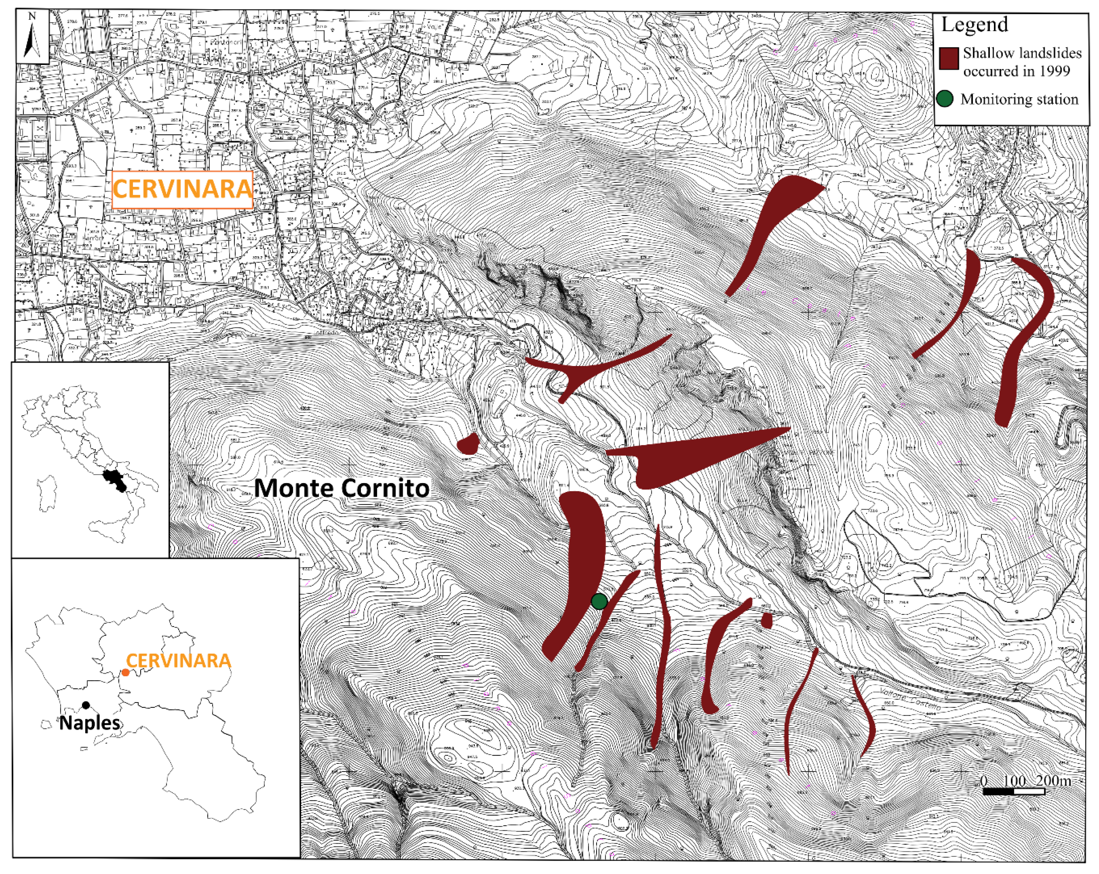
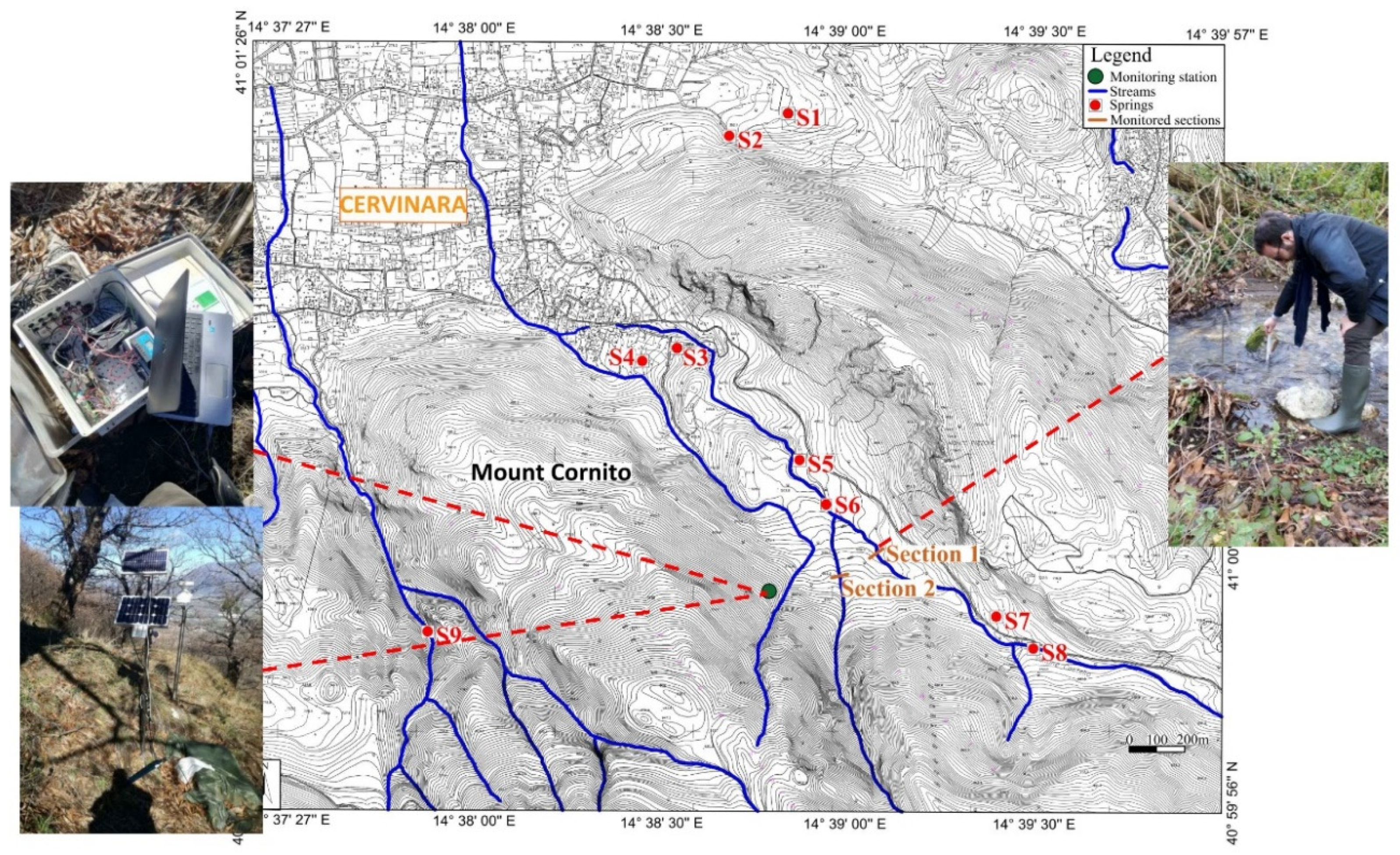
2.1. Study Area
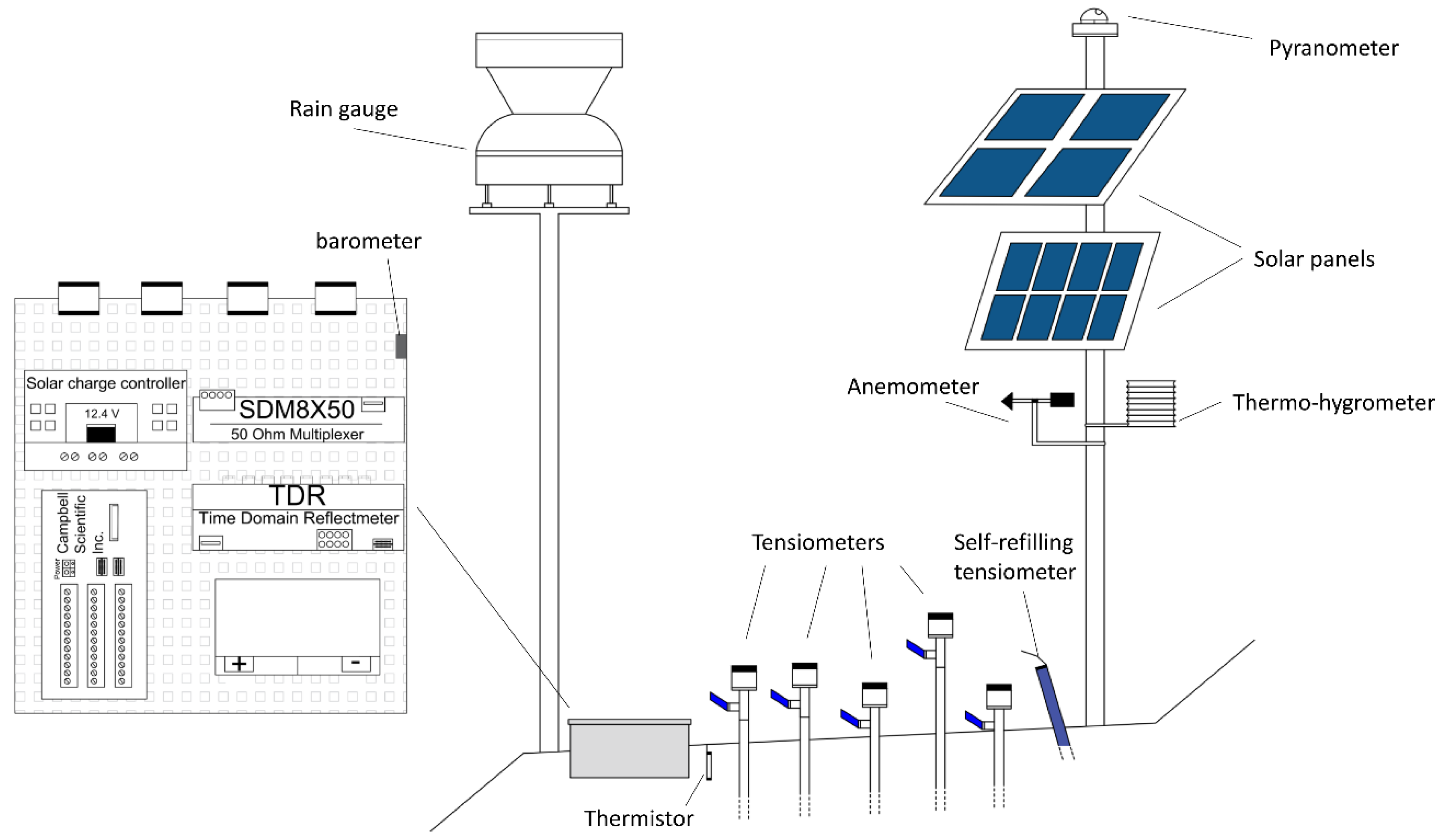
2.2. Hydro-Meteorological Monitoring Station
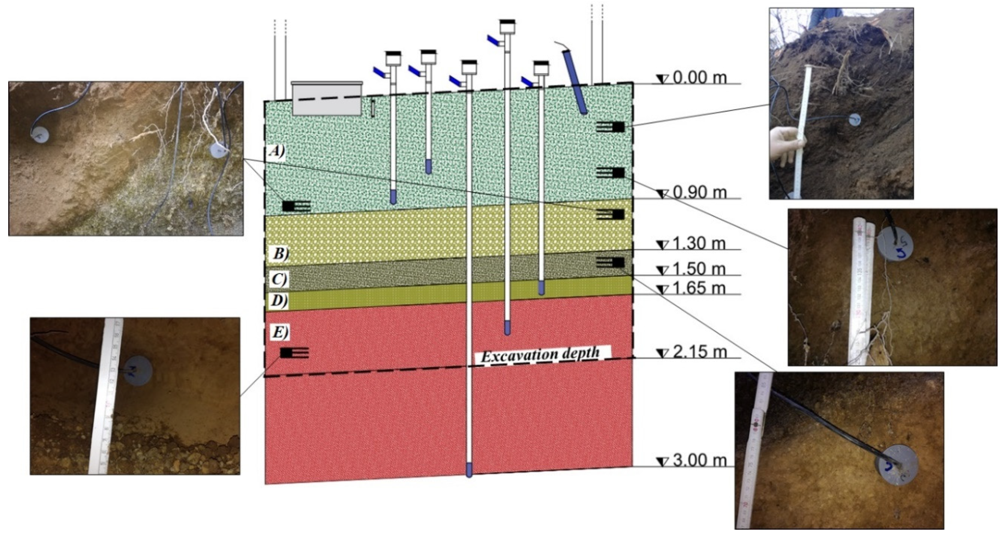
2.3. Surface and Groundwater Circulation
3. Monitoring Data
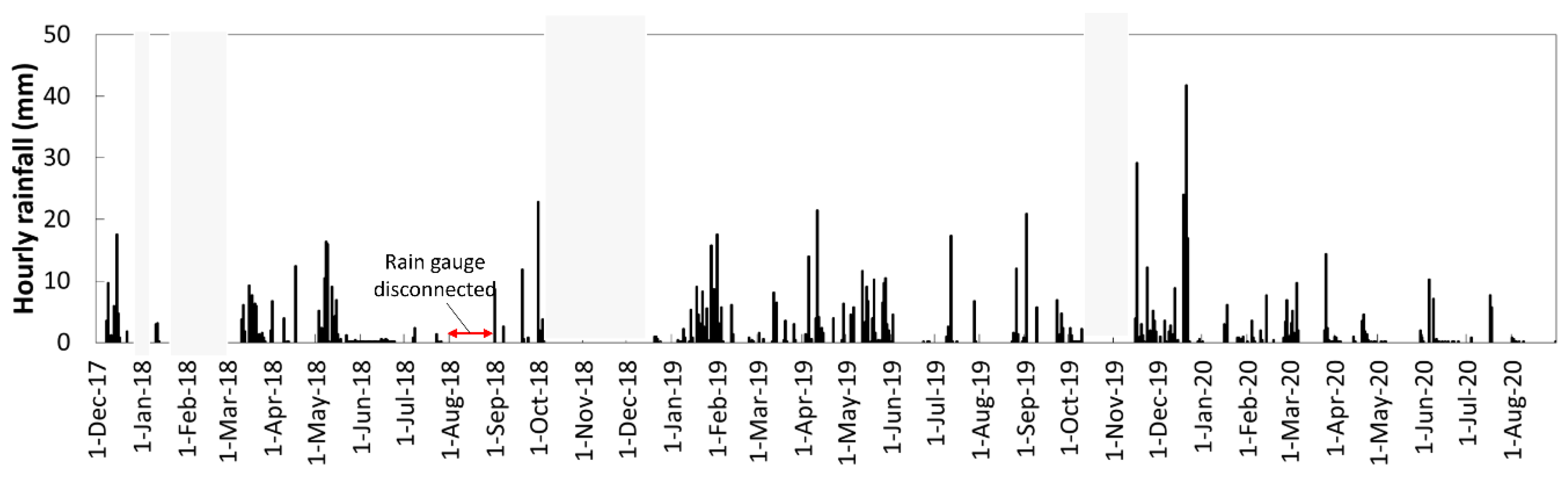
3.1. Precipitations
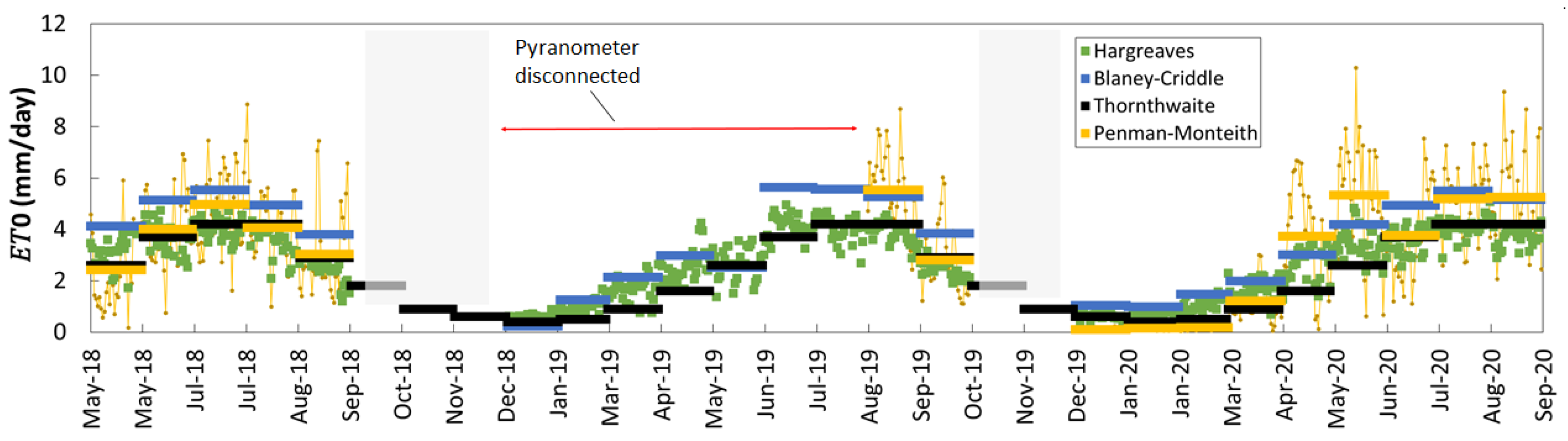
3.2. Evapotranspiration
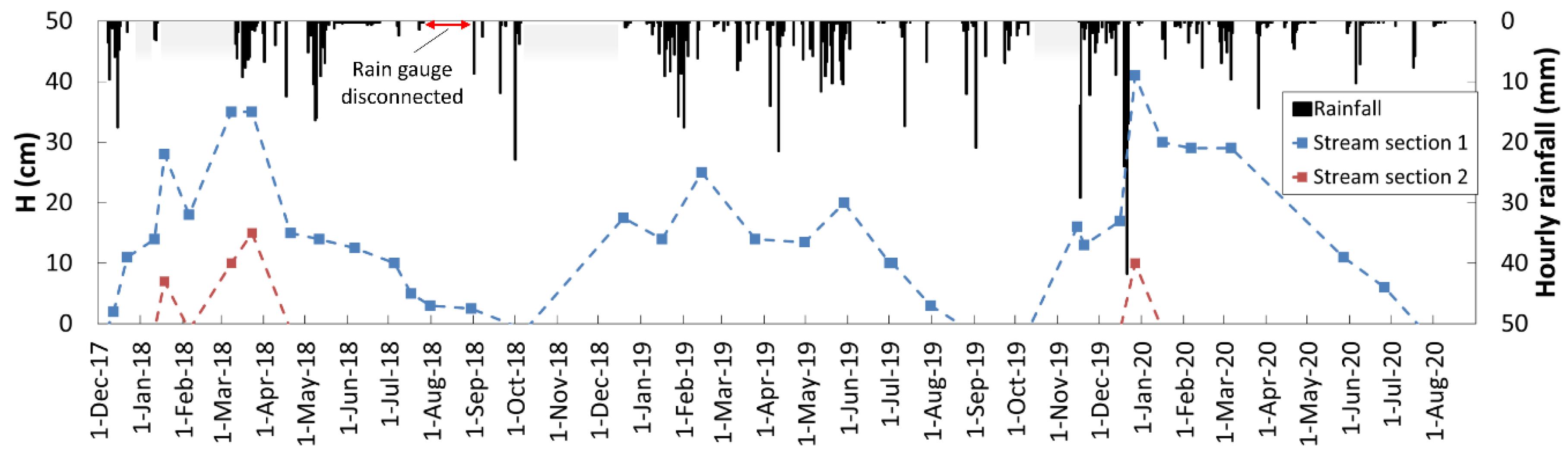
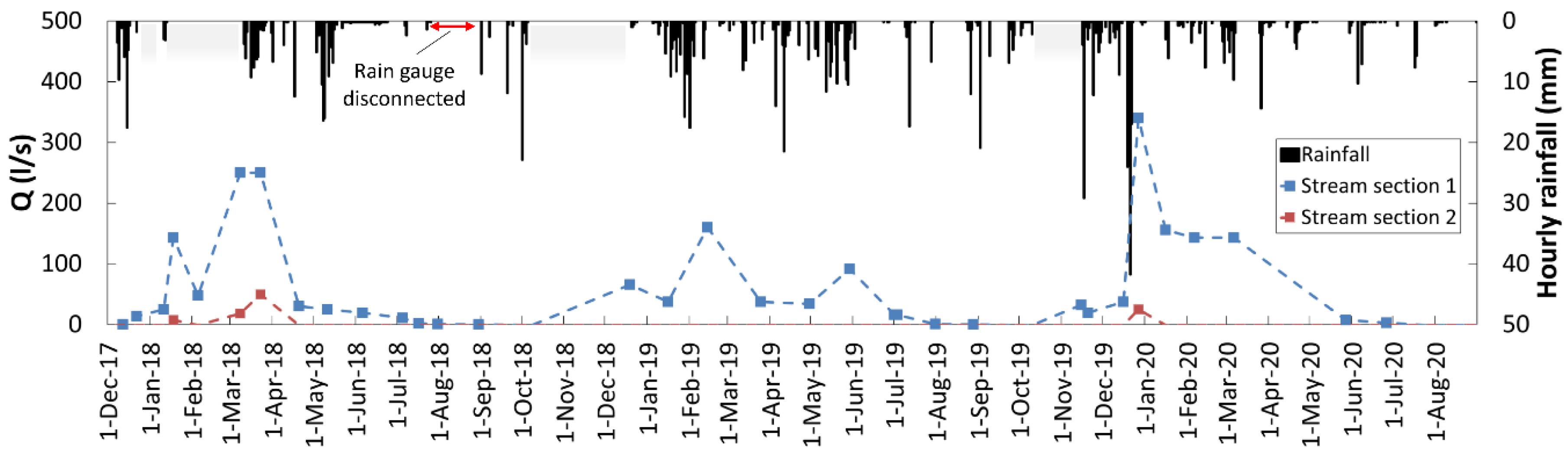
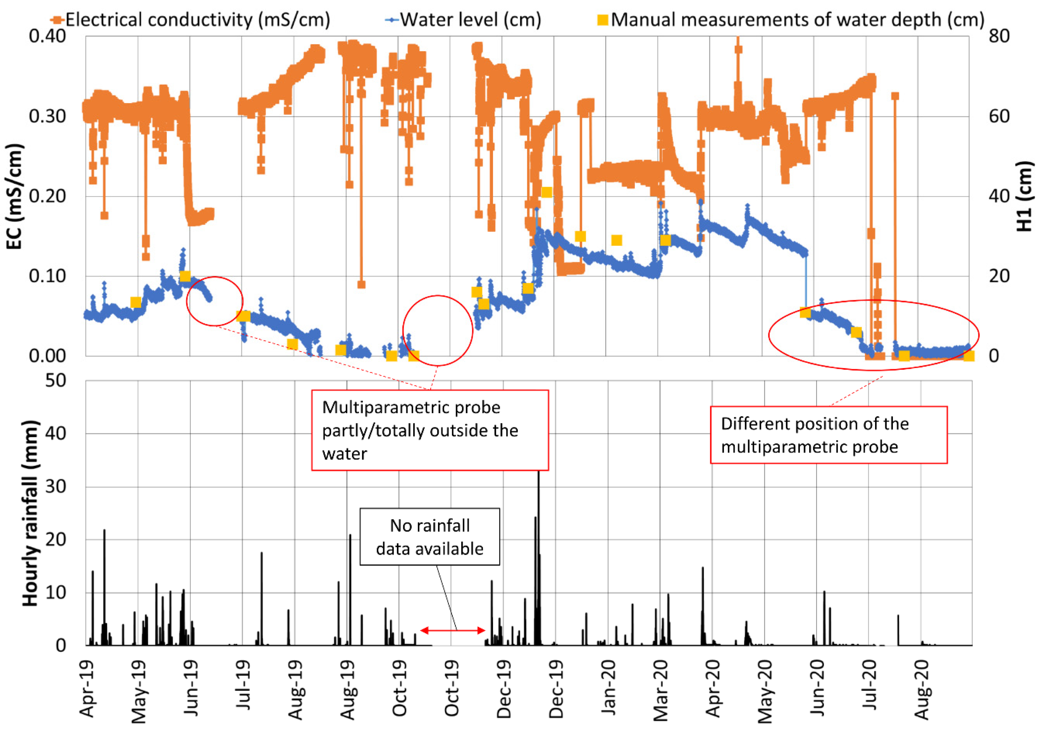
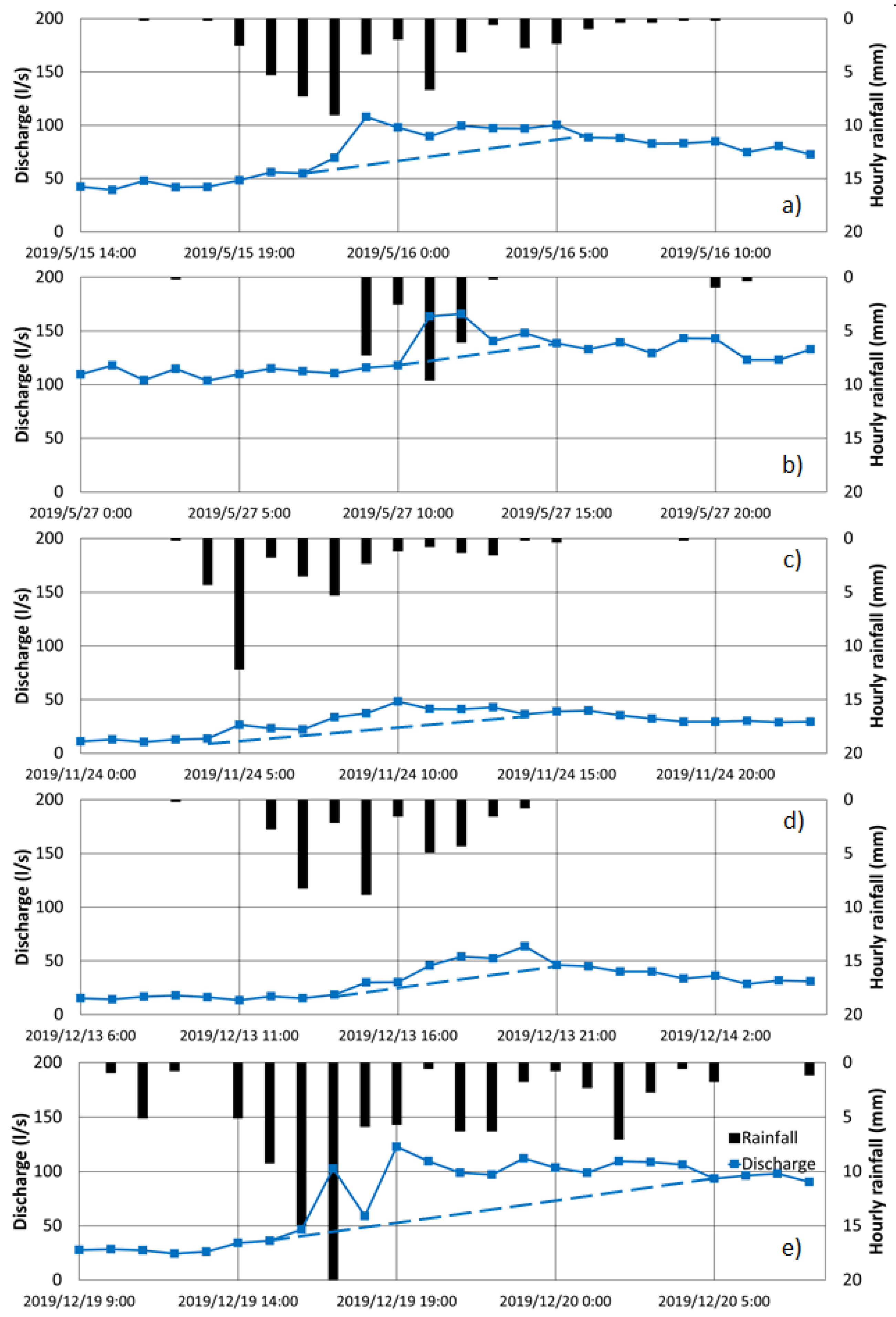
3.3. Stream Discharges
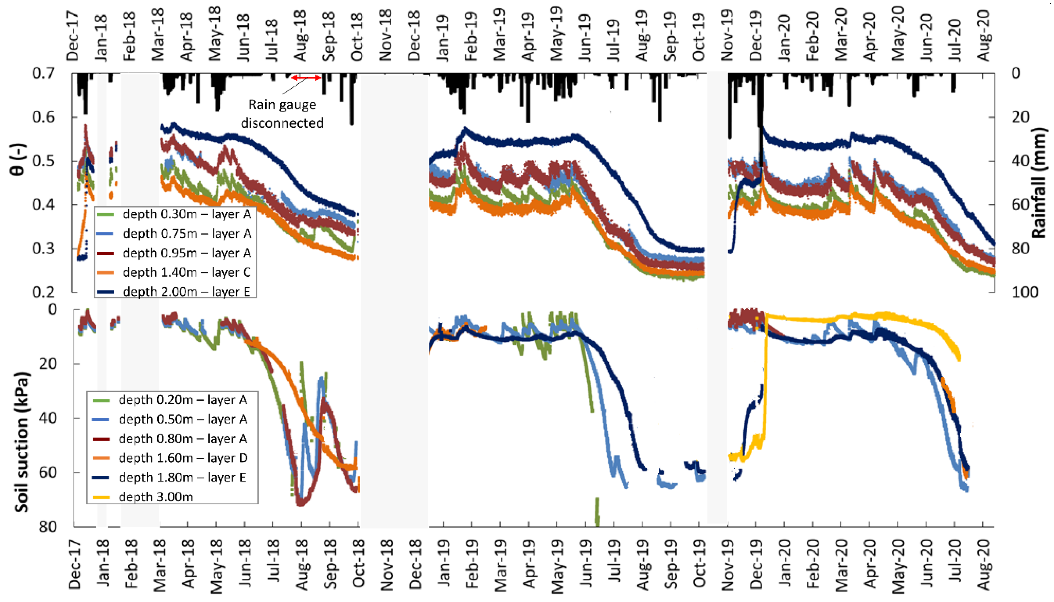
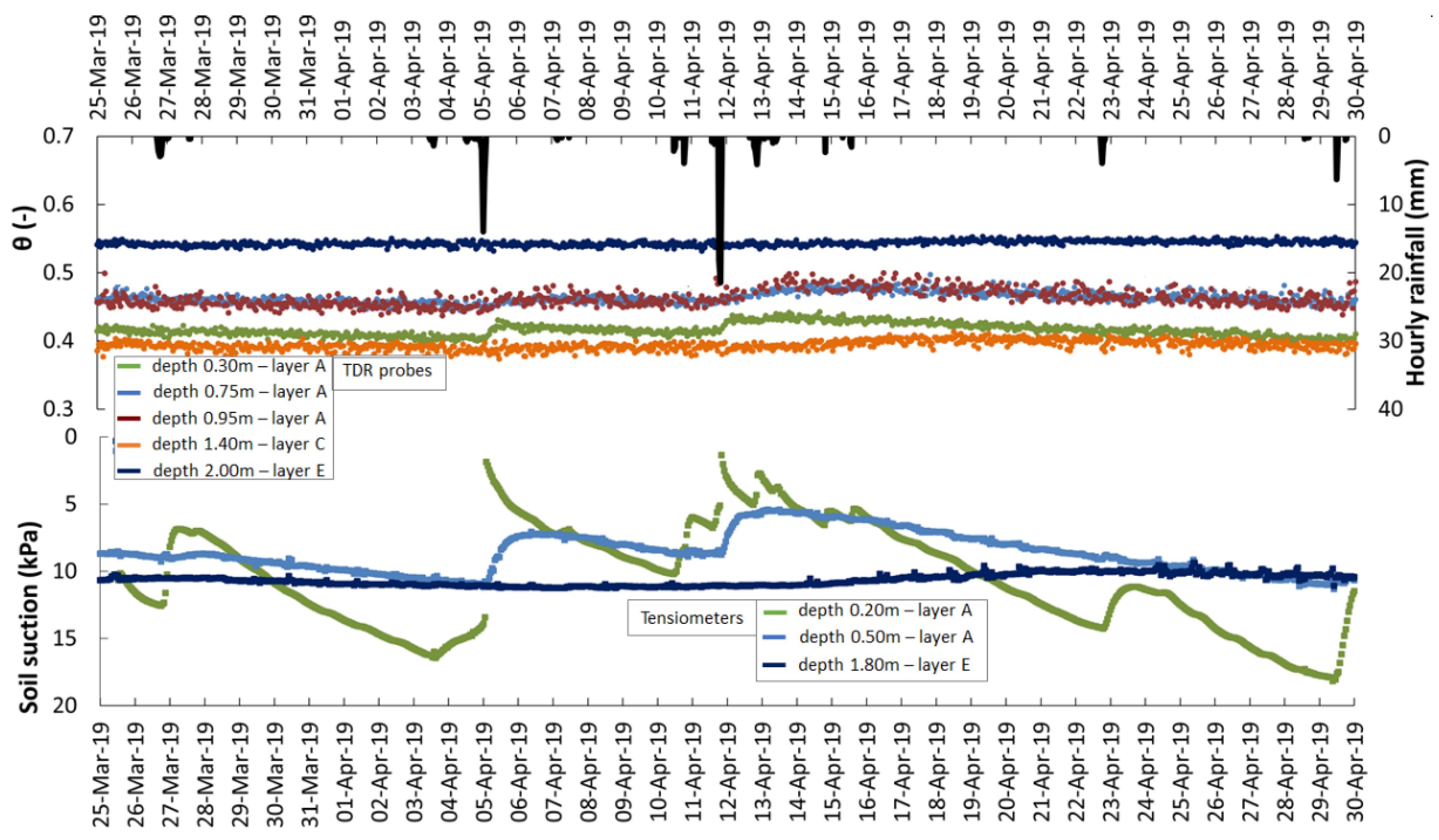
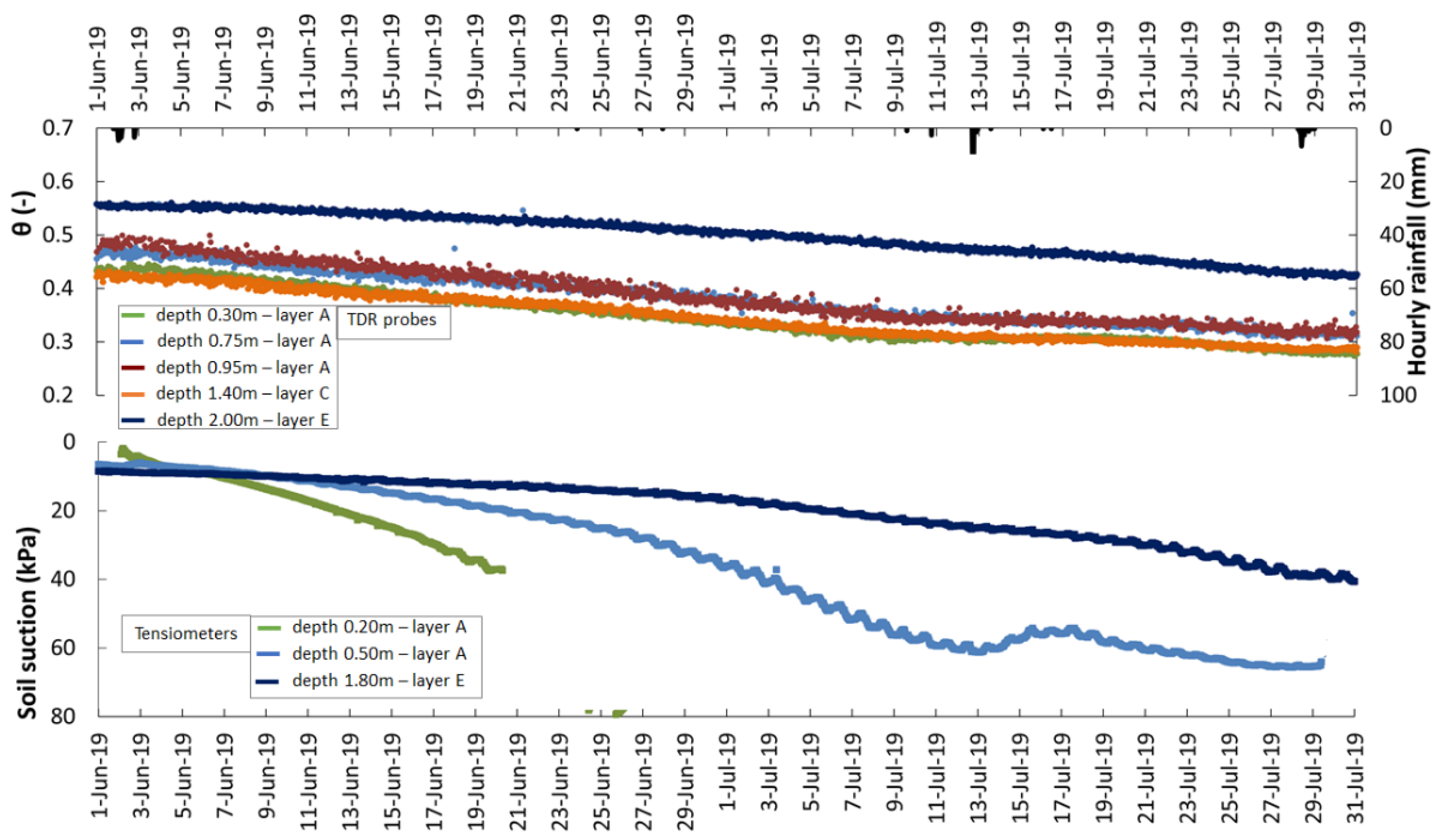
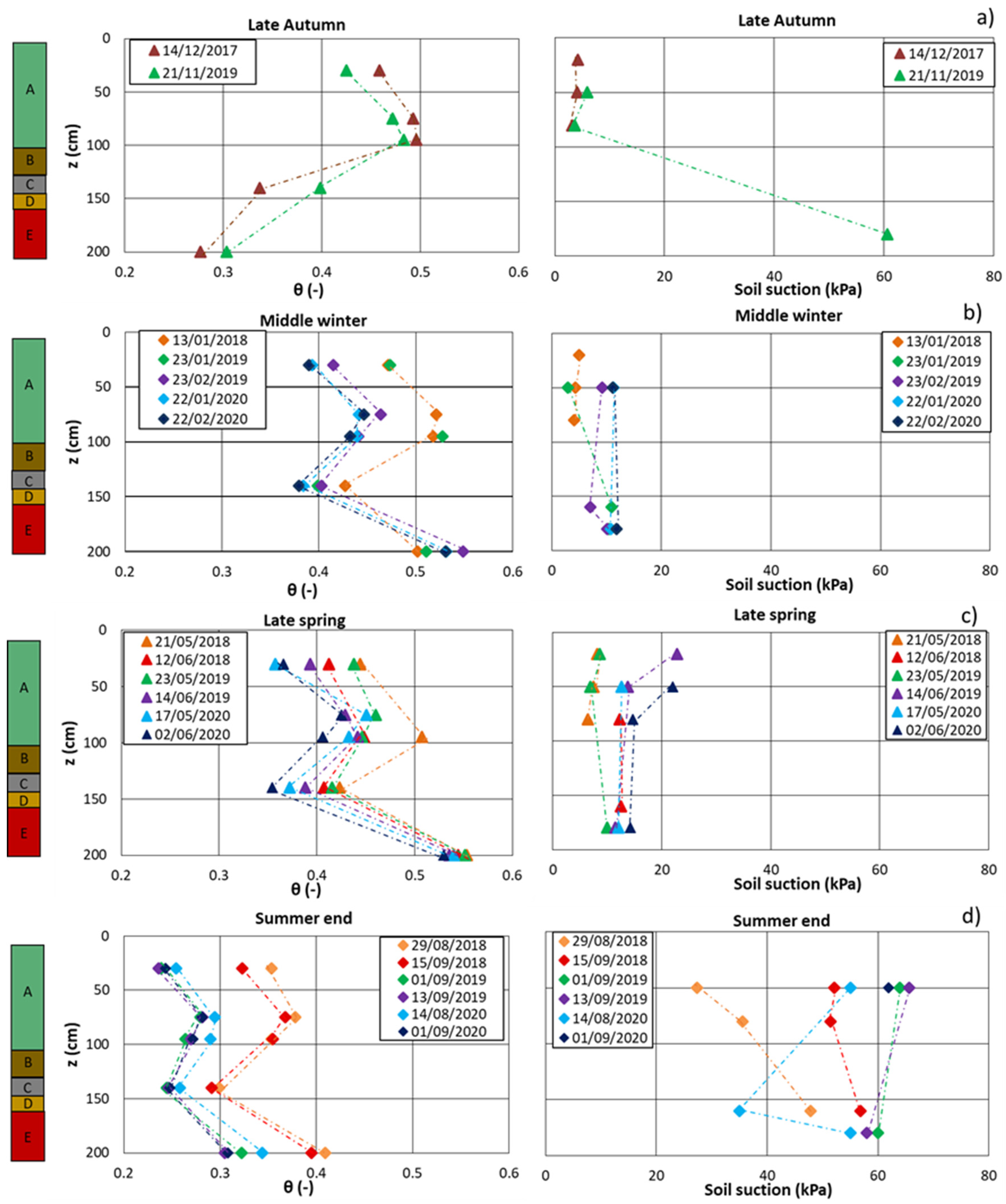
3.4. Soil Water Content and Suction
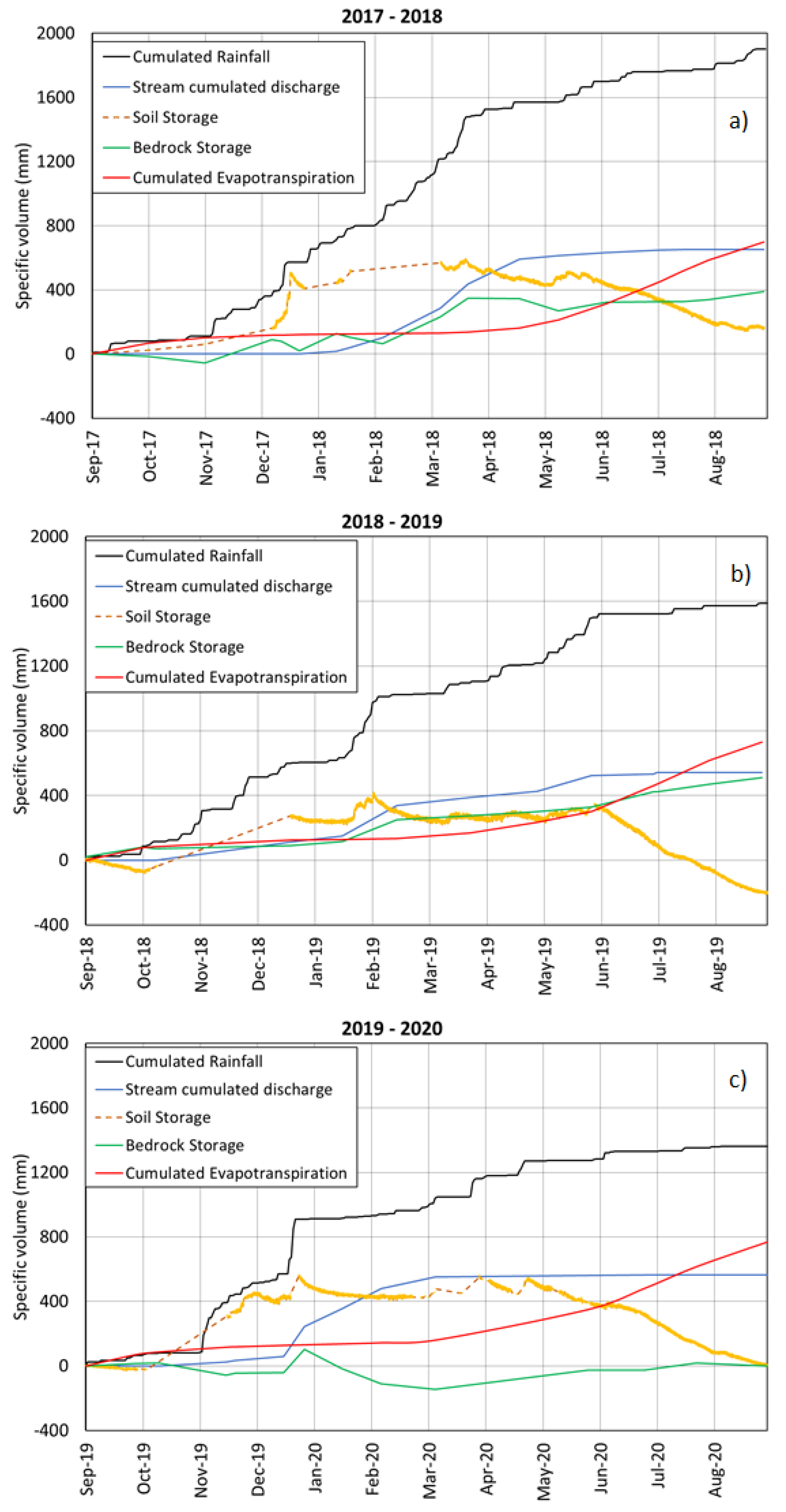
4. Discussion
5. Conclusions
Author Contributions
Funding
Acknowledgments
Conflicts of Interest
Data Availability
References
- Bogaard, T.A.; Greco, R. Landslide hydrology: From hydrology to pore pressure. Wiley Interdiscip. Rev. Water 2016, 3, 439–459. [Google Scholar] [CrossRef]
- Wieczorek, G.F.; Glade, T. Climatic factors influencing occurrence of debris flows. In Debris-Flow Hazards and Related Phenomena; Springer: Berlin/Heidelberg, Germany, 2007; pp. 325–362. [Google Scholar]
- Bogaard, T.A.; van Asch, T.W.J. The role of the soil moisture balance in the unsaturated zone on movement and stability of the Beline landslide, France. Earth Surf. Process. Landf. 2002, 27, 1177–1188. [Google Scholar] [CrossRef]
- Terlien, M.T.J. Hydrological landslide triggering in ash-covered slopes of Manizales (Columbia). Geomorphology 1997, 20, 165–175. [Google Scholar] [CrossRef]
- Von Ruette, J.; Lehmann, P.; Or, D. Effects of rainfall spatial variability and intermittency on shallow landslide triggering patterns at a catchment scale. Water Resour. Res. 2014, 50, 7780–7799. [Google Scholar] [CrossRef]
- Torres, R.; Dietrich, W.E.; Montgomery, D.R.; Anderson, S.P.; Loague, K. Unsaturated zone processes and the hydrologic response of a steep, unchanneled catchment. Water Resour. Res. 1998, 34, 1865–1879. [Google Scholar] [CrossRef]
- Johnson, K.A.; Sitar, N. Hydrologic conditions leading to debris-flow initiation. Can. Geotech. J. 1990, 27, 789–801. [Google Scholar] [CrossRef]
- Hidayat, R.; Sutanto, S.J.; Hidayah, A.; Ridwan, B.; Mulyana, A. Development of a Landslide Early Warning System in Indonesia. Geosciences 2019, 9, 451. [Google Scholar] [CrossRef] [Green Version]
- Chigira, M.; Kiho, K. Deep-seated rockslide-avalanches preceded by mass rock creep of sedimentary rocks in the Akaishi Mountains, central Japan. Eng. Geol. 1994, 38, 221–230. [Google Scholar] [CrossRef]
- Chigira, M. September 2005 rain-induced catastrophic rockslides on slopes affected by deep-seated gravitational deformations, Kyushu, southern Japan. Eng. Geol. 2009, 108. [Google Scholar] [CrossRef]
- Geertsema, M.; Clague, J.J.; Schwab, J.W.; Evans, S.G. An overview of recent large catastrophic landslides in northern British Columbia, Canada. Eng. Geol. 2006, 83, 120–143. [Google Scholar] [CrossRef]
- Agliardi, F.; Crosta, G.B.; Frattini, P. Slow rock-slope deformation. In Landslides; Clague, J.J., Stead, D., Eds.; Cambridge University Press: Cambridge, UK, 2013; pp. 207–221. [Google Scholar]
- Hungr, O.; Leroueil, S.; Picarelli, L. The Varnes classification of landslide types, an update. Landslides 2014, 11, 167–194. [Google Scholar] [CrossRef]
- Hutchinson, J.N. General report: Morphological and geotechnical parameters of landslides in relation to geology and hydrogeology. Int. J. Rock Mech. Min. Sci. Geomech. Abstr. 1989, 26, 88. [Google Scholar] [CrossRef]
- Bisci, C.; Burattini, F.; Dramis, F.; Leoperdi, S.; Pontoni, F.; Pontoni, F. The Sant’Agata Feltria landslide (Marche Region, central Italy): A case of recurrent earthflow evolving from a deep-seated gravitational slope deformation. Geomorphology 1996, 15, 351–361. [Google Scholar] [CrossRef]
- Tsou, C.-Y.; Feng, Z.-Y.; Chigira, M. Catastrophic landslide induced by Typhoon Morakot, Shiaolin, Taiwan. Geomorphology 2011, 127, 166–178. [Google Scholar] [CrossRef] [Green Version]
- Zerathe, S.; Lebourg, T. Evolution stages of large deep-seated landslides at the front of a subalpine meridional chain (Maritime-Alps, France). Geomorphology 2012, 138, 390–403. [Google Scholar] [CrossRef]
- Petley, D.N.; Allison, R.J. The mechanics of deep-seated landslides. Earth Surf. Process. Landf. 1997, 22, 747–758. [Google Scholar] [CrossRef]
- Ambrosi, C.; Crosta, G.B. Large sackung along major tectonic features in the Central Italian Alps. Eng. Geol. 2006, 83, 183–200. [Google Scholar] [CrossRef]
- Miller, D.J.; Dunne, T. Topographic perturbations of regional stresses and consequent bedrock fracturing. J. Geophys. Res. Solid Earth 1996, 101, 25523–25536. [Google Scholar] [CrossRef]
- Ambrosi, C.; Crosta, G.B. Valley shape influence on deformation mechanisms of rock slopes. Geol. Soc. London, Spec. Publ. 2011, 351, 215–233. [Google Scholar] [CrossRef]
- Moro, M.; Saroli, M.; Salvi, S.; Stramondo, S.; Doumaz, F. The relationship between seismic deformation and deep-seated gravitational movements during the 1997 Umbria–Marche (Central Italy) earthquakes. Geomorphology 2007, 89, 297–307. [Google Scholar] [CrossRef]
- Crosta, G. Landslide, spreading, deep seated gravitational deformation: Analysis, examples, problems and proposals. Geogr. Fis. E Din. Quat. 1997, 19, 297–313. [Google Scholar]
- Barla, G. Numerical modeling of deep-seated landslides interacting with man-made structures. J. Rock Mech. Geotech. Eng. 2018, 10, 1020–1036. [Google Scholar] [CrossRef]
- Padilla, C.; Onda, Y.; Iida, T.; Takahashi, S.; Uchida, T. Characterization of the groundwater response to rainfall on a hillslope with fractured bedrock by creep deformation and its implication for the generation of deep-seated landslides on Mt. Wanitsuka, Kyushu Island. Geomorphology 2014, 204, 444–458. [Google Scholar] [CrossRef]
- Lv, H.; Ling, C.; Hu, B.X.; Ran, J.; Zheng, Y.; Xu, Q.; Tong, J. Characterizing groundwater flow in a translational rock landslide of southwestern China. Bull. Eng. Geol. Environ. 2019, 78, 1989–2007. [Google Scholar] [CrossRef]
- Uchida, T.; Asano, Y.; Ohte, N.; Mizuyama, T. Seepage area and rate of bedrock groundwater discharge at a granitic unchanneled hillslope. Water Resour. Res. 2003, 39. [Google Scholar] [CrossRef]
- Jitousono, T.; Shimokawa, E.; Teramoto, Y. Debris flow induced by deep-seated landslides at Minamata City, kumamoto prefecture, Japan in 2003. Int. J. Eros. Control Eng. 2008, 1, 5–10. [Google Scholar] [CrossRef] [Green Version]
- Ebel, B.A.; Loague, K.; Montgomery, D.R.; Dietrich, W.E. Physics-based continuous simulation of long-term near-surface hydrologic response for the Coos Bay experimental catchment. Water Resour. Res. 2008, 44. [Google Scholar] [CrossRef]
- Crozier, M.J. Prediction of rainfall-triggered landslides: A test of the Antecedent Water Status Model. Earth Surf. Process. Landf. 1999, 24, 825–833. [Google Scholar] [CrossRef]
- Rahimi, A.; Rahardjo, H.; Leong, E.-C. Effect of antecedent rainfall patterns on rainfall-induced slope failure. J. Geotech. Geoenviron. Eng. 2011, 137, 483–491. [Google Scholar] [CrossRef]
- Marino, P.; Peres, D.J.; Cancelliere, A.; Greco, R.; Bogaard, T.A. Soil moisture information can improve shallow landslide forecasting using the hydrometeorological threshold approach. Landslides 2020, 17, 2041–2054. [Google Scholar] [CrossRef]
- Revellino, P.; Guadagno, F.M.; Hungr, O. Morphological methods and dynamic modelling in landslide hazard assessment of the Campania Apennine carbonate slope. Landslides 2008, 5, 59–70. [Google Scholar] [CrossRef]
- De Vita, P.; Agrello, D.; Ambrosino, F. Landslide susceptibility assessment in ash-fall pyroclastic deposits surrounding Mount Somma-Vesuvius: Application of geophysical surveys for soil thickness mapping. J. Appl. Geophys. 2006, 59, 126–139. [Google Scholar] [CrossRef]
- De Vita, P.; Napolitano, E.; Godt, J.W.; Baum, R.L. Deterministic estimation of hydrological thresholds for shallow landslide initiation and slope stability models: Case study from the Somma-Vesuvius area of southern Italy. Landslides 2013, 10, 713–728. [Google Scholar] [CrossRef]
- Del Soldato, M.; Segoni, S.; De Vita, P.; Pazzi, V.; Tofani, V.; Moretti, S. Thickness model of pyroclastic soils along mountain slopes of Campania (southern Italy). In Landslides and Engineered Slopes. Experience, Theory and Practice; CRC Press: Boca Raton, FL, USA, 2016; pp. 797–804. ISBN 9781138029880. [Google Scholar]
- Damiano, E.; Olivares, L. The role of infiltration processes in steep slope stability of pyroclastic granular soils: Laboratory and numerical investigation. Nat. Hazards 2010, 52, 329–350. [Google Scholar] [CrossRef]
- Guadagno, F.M.; Forte, R.; Revellino, P.; Fiorillo, F.; Focareta, M. Some aspects of the initiation of debris avalanches in the Campania Region: The role of morphological slope discontinuities and the development of failure. Geomorphology 2005, 66, 237–254. [Google Scholar] [CrossRef]
- Allocca, V.; Manna, F.; De Vita, P. Estimating annual groundwater recharge coefficient for karst aquifers of the southern Apennines (Italy). Hydrol. Earth Syst. Sci. 2014, 18, 803–817. [Google Scholar] [CrossRef] [Green Version]
- Perrin, J.; Jeannin, P.-Y.; Zwahlen, F. Epikarst storage in a karst aquifer: A conceptual model based on isotopic data, Milandre test site, Switzerland. J. Hydrol. 2003, 279, 106–124. [Google Scholar] [CrossRef]
- Hartmann, A.; Goldscheider, N.; Wagener, T.; Lange, J.; Weiler, M. Karst water resources in a changing world: Review of hydrological modeling approaches. Rev. Geophys. 2014, 52, 218–242. [Google Scholar] [CrossRef]
- Petrella, E.; Capuano, P.; Carcione, M.; Celico, F. A high-altitude temporary spring in a compartmentalized carbonate aquifer: The role of low-permeability faults and karst conduits. Hydrol. Process. 2009, 23, 3354–3364. [Google Scholar] [CrossRef]
- Bakalowicz, M. Epikarst. In Encyclopedia of Caves; Elsevier: Amsterdam, The Netherlands, 2012; pp. 284–288. [Google Scholar]
- Di Maio, R.; De Paola, C.; Forte, G.; Piegari, E.; Pirone, M.; Santo, A.; Urciuoli, G. An integrated geological, geotechnical and geophysical approach to identify predisposing factors for flowslide occurrence. Eng. Geol. 2020, 267, 105473. [Google Scholar] [CrossRef]
- Celico, F.; Naclerio, G.; Bucci, A.; Nerone, V.; Capuano, P.; Carcione, M.; Allocca, V.; Celico, P. Influence of pyroclastic soil on epikarst formation: A test study in southern Italy. Terra Nov. 2010, 22, 110–115. [Google Scholar] [CrossRef]
- Cascini, L.; Sorbino, G.; Cuomo, S.; Ferlisi, S. Seasonal effects of rainfall on the shallow pyroclastic deposits of the Campania region (southern Italy). Landslides 2014, 11, 779–792. [Google Scholar] [CrossRef]
- Comegna, L.; Damiano, E.; Greco, R.; Guida, A.; Olivares, L.; Picarelli, L. Field hydrological monitoring of a sloping shallow pyroclastic deposit. Can. Geotech. J. 2016, 53, 1125–1137. [Google Scholar] [CrossRef] [Green Version]
- Greco, R.; Marino, P.; Santonastaso, G.F.; Damiano, E. Interaction between perched epikarst aquifer and unsaturated soil cover in the initiation of shallow landslides in pyroclastic soils. Water 2018, 10, 948. [Google Scholar] [CrossRef] [Green Version]
- Marino, P.; Santonastaso, G.F.; Fan, X.; Greco, R. Prediction of shallow landslides in pyroclastic-covered slopes by coupled modeling of unsaturated and saturated groundwater flow. Landslides 2020. [Google Scholar] [CrossRef]
- Fusco, F.; De Vita, P.; Mirus, B.B.; Baum, R.L.; Allocca, V.; Tufano, R.; Di Clemente, E.; Calcaterra, D. Physically based estimation of rainfall thresholds triggering shallow landslides in volcanic slopes of southern Italy. Water 2019, 11, 1915. [Google Scholar] [CrossRef] [Green Version]
- Trandafir, A.C.; Sidle, R.C.; Gomi, T.; Kamai, T. Monitored and simulated variations in matric suction during rainfall in a residual soil slope. Environ. Geol. 2008, 55, 951–961. [Google Scholar] [CrossRef]
- Tsaparas, I.; Rahardjo, H.; Toll, D.G.; Leong, E.-C. Infiltration characteristics of two instrumented residual soil slopes. Can. Geotech. J. 2003, 40, 1012–1032. [Google Scholar] [CrossRef]
- Hawke, R.; McConchie, J. In situ measurement of soil moisture and pore-water pressures in an ‘incipient’ landslide: Lake Tutira, New Zealand. J. Environ. Manag. 2011, 92, 266–274. [Google Scholar] [CrossRef]
- Damiano, E.; Olivares, L.; Picarelli, L. Steep-slope monitoring in unsaturated pyroclastic soils. Eng. Geol. 2012, 137–138, 1–12. [Google Scholar] [CrossRef]
- Papa, R.; Urciuoli, G.; Evangelista, A.; Nicotera, M. Field investigation on triggering mechanisms of fast landslides in unsaturated pyroclastic soils. In Unsaturated Soils. Advances in Geo-Engineering; Taylor & Francis: Abingdon, UK, 2008; pp. 909–915. ISBN 0415476925. [Google Scholar]
- Pirone, M.; Papa, R.; Nicotera, M. Test site experience on mechanisms triggering mudflows in unsaturated pyroclastic soils in southern Italy. In Unsaturated Soils; CRC Press: Boca Raton, FL, USA, 2010; pp. 1273–1278. ISBN 9780415604307. [Google Scholar]
- Kosugi, K.; Katsura, S.; Katsuyama, M.; Mizuyama, T. Water flow processes in weathered granitic bedrock and their effects on runoff generation in a small headwater catchment. Water Resour. Res. 2006, 42. [Google Scholar] [CrossRef]
- Salve, R.; Rempe, D.M.; Dietrich, W.E. Rain, rock moisture dynamics, and the rapid response of perched groundwater in weathered, fractured argillite underlying a steep hillslope. Water Resour. Res. 2012, 48. [Google Scholar] [CrossRef]
- Brönnimann, C.; Stähli, M.; Schneider, P.; Seward, L.; Springman, S.M. Bedrock exfiltration as a triggering mechanism for shallow landslides. Water Resour. Res. 2013, 49, 5155–5167. [Google Scholar] [CrossRef] [Green Version]
- Fiorillo, F.; Guadagno, F.; Aquino, S.; De Blasio, A. The December 1999 Cervinara landslides: Further debris flows in the pyroclastic deposits of Campania (southern Italy). Bull. Eng. Geol. Environ. 2001, 60, 171–184. [Google Scholar] [CrossRef]
- Comegna, L.; Damiano, E.; Greco, R.; Guida, A.; Olivares, L.; Picarelli, L. Effects of the vegetation on the hydrological behavior of a loose pyroclastic deposit. Procedia Environ. Sci. 2013, 19, 922–931. [Google Scholar] [CrossRef] [Green Version]
- Greco, R.; Comegna, L.; Damiano, E.; Guida, A.; Olivares, L.; Picarelli, L. Hydrological modelling of a slope covered with shallow pyroclastic deposits from field monitoring data. Hydrol. Earth Syst. Sci. 2013, 17, 4001–4013. [Google Scholar] [CrossRef] [Green Version]
- Rolandi, G.; Bellucci, F.; Heizler, M.T.; Belkin, H.E.; De Vivo, B. Tectonic controls on the genesis of ignimbrites from the Campanian Volcanic Zone, southern Italy. Mineral. Petrol. 2003, 79, 3–31. [Google Scholar] [CrossRef]
- Greco, R.; Guida, A. Field measurements of topsoil moisture profiles by vertical TDR probes. J. Hydrol. 2008, 348, 442–451. [Google Scholar] [CrossRef]
- Topp, G.C.; Davis, J.L.; Annan, A.P. Electromagnetic determination of soil water content: Measurements in coaxial transmission lines. Water Resour. Res. 1980, 16, 574–582. [Google Scholar] [CrossRef] [Green Version]
- Capparelli, G.; Spolverino, G.; Greco, R. Experimental Determination of TDR Calibration Relationship for Pyroclastic Ashes of Campania (Italy). Sensors 2018, 18, 3727. [Google Scholar] [CrossRef] [Green Version]
- Greco, R.; Guida, A.; Damiano, E.; Olivares, L. Soil water content and suction monitoring in model slopes for shallow flowslides early warning applications. Phys. Chem. Earth Parts A/B/C 2010, 35, 127–136. [Google Scholar] [CrossRef]
- McDonnell, J.J.; Stewart, M.K.; Owens, I.F. Effect of catchment-scale subsurface mixing on stream isotopic response. Water Resour. Res. 1991, 27, 3065–3073. [Google Scholar] [CrossRef]
- Pellerin, B.A.; Wollheim, W.M.; Feng, X.; Vörösmarty, C.J. The application of electrical conductivity as a tracer for hydrograph separation in urban catchments. Hydrol. Process. 2008, 22, 1810–1818. [Google Scholar] [CrossRef]
- Pearce, A.J.; Stewart, M.K.; Sklash, M.G. Storm runoff generation in humid headwater catchments: 1. Where does the water come from? Water Resour. Res. 1986, 22, 1263–1272. [Google Scholar] [CrossRef]
- Hargreaves, G.H.; Allen, R.G. History and evaluation of hargreaves evapotranspiration equation. J. Irrig. Drain. Eng. 2003, 129, 53–63. [Google Scholar] [CrossRef]
- Blaney, H.F.; Criddle, W.D. Determining Consumptive Use and Irrigation Water Requirements; US Department of Agriculture: Washington, DC, USA, 1962.
- Doorenbos, J.; Pruitt, W.O. Crop Water Requirements; FAO Irrigation and Drainage Paper 24; FAO: Rome, Italy, 1977; ISBN 9251002797. [Google Scholar]
- Monteith, J.L. Evaporation and environment. In Symposia of the Society for Experimental Biology; Cambridge University Press: Cambridge, UK, 1965. [Google Scholar]
- Thornthwaite, C.W. An Approach toward a Rational Classification of Climate. Geogr. Rev. 1948, 38, 55. [Google Scholar] [CrossRef]
- Breuer, L.; Eckhardt, K.; Frede, H.-G. Plant parameter values for models in temperate climates. Ecol. Modell. 2003, 169, 237–293. [Google Scholar] [CrossRef]
- Cutini, A.; Matteucci, G.; Mugnozza, G.S. Estimation of leaf area index with the Li-Cor LAI 2000 in deciduous forests. For. Ecol. Manag. 1998, 105, 55–65. [Google Scholar] [CrossRef]
- Körner, C.; Ja, S. Maximum leaf diffusive conductance in vascular plants. Photosynthetica 1979, 13, 45–82. [Google Scholar]
- Shuttleworth, W.J. Evaporation. In Handbook of Hydrology; Maidment, D.R., Ed.; McGraw-Hill: New York, NY, USA, 1993; ISBN 0070397325. [Google Scholar]
- Testa, G.; Gresta, F.; Cosentino, S.L. Dry matter and qualitative characteristics of alfalfa as affected by harvest times and soil water content. Eur. J. Agron. 2011, 34, 144–152. [Google Scholar] [CrossRef]
- Allen, R.G.; Pereira, L.S.; Smith, M.; Raes, D.; Wright, J.L. FAO-56 dual crop coefficient method for estimating evaporation from soil and application extensions. J. Irrig. Drain. Eng. 2005, 131, 2–13. [Google Scholar] [CrossRef] [Green Version]
- Pirone, M.; Papa, R.; Nicotera, M.V.; Urciuoli, G. Evaluation of the hydraulic hysteresis of unsaturated pyroclastic soils by in situ measurements. Procedia Earth Planet. Sci. 2014, 9, 163–170. [Google Scholar] [CrossRef] [Green Version]
- De Vita, P.; Fusco, F.; Tufano, R.; Cusano, D. Seasonal and event-based hydrological and slope stability modeling of pyroclastic fall deposits covering slopes in Campania (Southern Italy). Water 2018, 10, 1140. [Google Scholar] [CrossRef] [Green Version]


| ELETRONIC SENSORS | COMPANY | MODEL | MEASUREMENT RANGE | TEMPERATURE RANGE | ACCURACY | |
|---|---|---|---|---|---|---|
| 1 | Data logger and data Acquisition System | Campbell Scientific Inc. * | CR-1000 | - | −25 °C to + 50 °C (standard) | ± (0.06% of reading + offset) at 0 °C to 40 °C for Analog Voltage |
| 2 | Time- Domain Reflectometer | Campbell Scientific Inc. * | TDR-100 | −2 m to 2100 m (distance) and 0 to 7 µs (time) | −40 °C to + 55 °C | - |
| 3 | Multiplexer for TDR System | Campbell Scientific Inc. * | SDM8 × 50 | 8-Channel | −40 °C to + 55 °C | - |
| 4 | Tension Transducer | Soil Moisture Equipment Corp. ** | 5301 | 0–85 cBar | 0 °C to + 60 °C | 0.25% |
| 5 | Self-refilling Tensiometer | METER Group, Inc. *** | TS1 | 0–85 kPa | −30 °C to + 70 °C | ±0.5 kPa (Soil water tension) ±0.4 K (Temperature) |
| 6 | Rain gauge | Campbell Scientific Inc. * | ARG100 | 0–500 mm/hr | - | - |
| 7 | Thermo-hygrometer (Air Temperature) | Campbell Scientific Inc. * | CS215 | −40 °C to + 70 °C | −40 °C to + 70 °C | ±0.3 °C (25 °C) ±0.4 °C (5 °C to 40 °C) ±0.9 °C (−40 °C to +70 °C) |
| 8 | Thermo-hygrometer (Relative humidity) | Campbell Scientific Inc. * | CS215 | 0 to 100% (−20 °C to +60 °C) | −40 °C to + 70 °C | ±2% (10% to 90% range) at 25 °C ±4% (0% to 100% range) at 25 °C |
| 9 | Thermistor | Campbell Scientific Inc. | 107 | −35 °C to +50 °C | −35 °C to + 50 °C | 0.3 °C |
| 10 | Anemometer | Campbell Scientific Inc. * | WSS2 | 0–90 m/s | −20 °C to + 70 °C | 2% |
| 11 | Pyranometer | Campbell Scientific Inc. * | SP110 | 0–1750 W/m2 | −40 °C to + 70 °C | ±5% |
| 12 | Barometer | Campbell Scientific Inc. * | SB-100 | 15–115 kpa | −40 °C to + 125 °C | ±1.5% |
| Number | Springs | Area | Regime |
|---|---|---|---|
| S1 | Vullo | Valle | perennial |
| S2 | Fontanastella | Valle | perennial |
| S3 | Ricci | Castello | perennial |
| S4 | Santospirito | Ioffredo | perennial |
| S5 | Pastore | Castello | seasonal |
| S6 | Acquerosse | Montepizzone | seasonal |
| S7 | Pisciariello 1 | Montepizzone | perennial |
| S8 | Pisciariello 2 | Foresta | perennial |
| S9 | Livera | Piano Gregorio | seasonal |
| 1. Hargreaves (mm/day) | ||
| = mean daily air temperature | (°C) | * |
| = extraterrestrial radiation | (mm/day) | - |
| 2. Blaney–Criddle (mm/day) | ||
| = daily minimum relative humidity | (%) | * |
| = daily wind speed at 2 m above the ground | (m/s) | * |
| = ratio between monthly average daily bright sunshine duration n(h) and monthly average maximum daily sunshine duration N(h) | (-) | 0.7 |
| p = mean daily percentage of annual daylight hours for a given month | (%) | |
| T = mean monthly air temperature | (°C) | * |
| 3. Penman–Monteith (mm/day) | ||
| λ = latent heat of vaporisation of water | (MJ/kg) | 2.45 |
| = slope of the saturation vapor pressure-temperature relationship, d/dT | (kPa/°C) | |
| = mean daily air temperature | (°C) | * |
| A= Available energy | (MJ/m2 day) | -G–P |
| = net radiation flux | (1–α) R* | |
| G = soil heat flux | - | |
| P = energy absorbed by biochemical process in the plants | 2% | |
| = density of moist air | (kPa/m3) | |
| = specific heat of moist air | (MJ/kg °C) | 0.001013 |
| D = vapour pressure deficit | (kPa) | |
| = mean saturated vapor pressure | (kPa) | |
| = mean actual vapor pressure | (kPa) | |
| γ = psychometric constant | (kPa/°C) | |
| rs = surface resistance to vapor emission by the stomata of leaves | (s/m) | 200/(LAI) |
| ra = aerodynamic resistance to upward vapor diffusion | (s/m) | |
| = elevation of wind speed measured | (m) | 2 |
| = vegetation height | (m) | 18 |
| 4. Thornthwaite (mm/month) | ||
| = average daily air temperature for a given month | (°C) | *** |
| L = monthly average maximum daily bright sunshine duration | hour | ** |
| N = number of days for a given month | (-) | |
| Year | ET0 (mm) | ET (mm) |
|---|---|---|
| 2017–2018 | 911.3 | 734.3 |
| 2018–2019 | 1000.3 | 781.0 |
| 2019–2020 | 1021.6 | 793.2 |
| Event | Data | Total Precipitation Depth (mm) | Total Specific Flood Runoff Volume (mm) | Runoff Coefficient (%) |
|---|---|---|---|---|
| (a) | 15 May 2019 | 45.1 | 0.487 | 1.08 |
| (b) | 27 May 2019 | 25.6 | 0.253 | 0.98 |
| (c) | 24 November 2019 | 34.5 | 0.217 | 0.63 |
| (d) | 13 December 2019 | 35.3 | 0.197 | 0.56 |
| (e) | 19 December 2019 | 102.2 | 1.038 | 1.02 |
| Months | Oct | Nov | Dec | Jan | Feb | Mar | Apr | May | Jun | Jul | Aug | Sep |
|---|---|---|---|---|---|---|---|---|---|---|---|---|
| Seasons * | wet | dry | ||||||||||
| This study ** | Late autumn 1 | Middle winter 2 | Late spring 3 | Summer end 4 | ||||||||
Publisher’s Note: MDPI stays neutral with regard to jurisdictional claims in published maps and institutional affiliations. |
© 2020 by the authors. Licensee MDPI, Basel, Switzerland. This article is an open access article distributed under the terms and conditions of the Creative Commons Attribution (CC BY) license (http://creativecommons.org/licenses/by/4.0/).
Share and Cite
Marino, P.; Comegna, L.; Damiano, E.; Olivares, L.; Greco, R. Monitoring the Hydrological Balance of a Landslide-Prone Slope Covered by Pyroclastic Deposits over Limestone Fractured Bedrock. Water 2020, 12, 3309. https://doi.org/10.3390/w12123309
Marino P, Comegna L, Damiano E, Olivares L, Greco R. Monitoring the Hydrological Balance of a Landslide-Prone Slope Covered by Pyroclastic Deposits over Limestone Fractured Bedrock. Water. 2020; 12(12):3309. https://doi.org/10.3390/w12123309
Chicago/Turabian StyleMarino, Pasquale, Luca Comegna, Emilia Damiano, Lucio Olivares, and Roberto Greco. 2020. "Monitoring the Hydrological Balance of a Landslide-Prone Slope Covered by Pyroclastic Deposits over Limestone Fractured Bedrock" Water 12, no. 12: 3309. https://doi.org/10.3390/w12123309