Analysis of Spatiotemporal Variability of Corn Yields Using Empirical Orthogonal Functions

1
Environmental Microbial and Food Safety Laboratory, USDA-ARS, Beltsville, MD 20705, USA
2
Hydrology and Remote Sensing Laboratory, USDA-ARS, Beltsville, MD 20705, USA
3
Centro Las Torres-Tomejil, IFAPA, 41200 Sevilla, Spain
*
Author to whom correspondence should be addressed.
Water 2020, 12(12), 3339; https://doi.org/10.3390/w12123339
Submission received: 26 October 2020
/
Revised: 21 November 2020
/
Accepted: 25 November 2020
/
Published: 28 November 2020
(This article belongs to the Special Issue Soil–Plant–Water Dynamics on a Field Scale)
Abstract
:We used empirical orthogonal functions (EOF) to analyze the spatial and temporal patterns of corn (Zea mays L.) yields at three hydrologically-bounded fields with shallow subsurface preferential lateral flow pathways. One field received uniform application of manure, the second field received the uniform applications of the chemical nitrogen fertilizer, and the third field received variable rate applications of the chemical fertilizer. The preferential subsurface flow and storage pathway locations were inferred from the ground penetration radar survey. Six-year monitoring data were analyzed. Statistical distributions of EOFs across fields were approximately symmetrical. Semivariograms of the first EOF differed between fields receiving manure and chemical fertilizer. This EOF accounted for 52 to 56% of the interannual variability of yields, and its values reflected the distance to the subsurface flow and storage pathways. The second and third EOF explained 17 to 20% and 10 to 13% of the interannual variability of yields, respectively. The precision applications of the nitrogen fertilizer minimized corn yield variability associated with subsurface preferential flow patterns. Investigating spatial patterns of yield variability under shallow groundwater flow control can be beneficial for the within-field crop management resource allocation.
1. Introduction
Crop yields vary spatially and temporally. Understanding variability is important for efficient use of farm resources [1]. Multiyear observations often show that some sections of fields are less productive than other sections. This has been attributed to the spatial variation of soil fertility [2], the ability of soil to retain and transmit water [3], and interactions of the above and other environmental factors [4].
The proximity of groundwater and the capillary fringe to the soil surface and root systems can be an important control of the crop yield. It has been demonstrated that the groundwater depth in the range from one to three meters created favorable conditions for corn crop, whereas groundwater depth less than one meter affected corn yields negatively [5,6]. The groundwater proximity and flow affect water availability that can be very important in dry years or areas, transport and availability of nutrients when water availability is not restrictive factor of crop yields, and loss of nitrogen to denitrification that can be important in wet years or areas. Continuous low-permeability layers in or below soil profiles may cause the existence of subsurface networks of predominantly lateral flow pathways [7,8]. Tromp-Van Meerveld and McDonnell (2006) noted that networks of such lateral flow pathways on the bedrock surface are dynamic, and some of their segments may exist for some time as subsurface mini ponds—i.e., groundwater lenses located in depressions and isolated from the rest of the network until the rainfall water infiltrates and overfills these depressions causing water to “spill” downslope [9].
Successful quantification of spatio-temporal variability of environmental variables in soil-plant-atmosphere systems has revealed spatial patterns that are temporally stable—i.e., change little over the observation period [10]. The principal component analysis is among the efficient techniques in determining patterns in spatio-temporal data. Patterns found by using this type of analysis are called empirical orthogonal functions (EOFs): they have been used in a broad range of environmental studies [11,12]. Usually, a small number of EOFs can explain the bulk of the observed variability. Interpreting EOFs as the manifestation of environmental factors provided the guidance for realistic forecasting of crop yields at large scales [13,14,15]. A better understanding of crop yield patterns is also required at field scales. Knowing yield spatial patterns that are stable over several years can improve long term management strategies [16]. However, EOF analysis has not been applied for that purpose to date. Our objective was to evaluate EOFs of multiyear crop yield data for detecting differences in access to shallow groundwater and nutrient management across cornfields of an intensively monitored experimental site.
2. Materials and Methods
2.1. Site Description
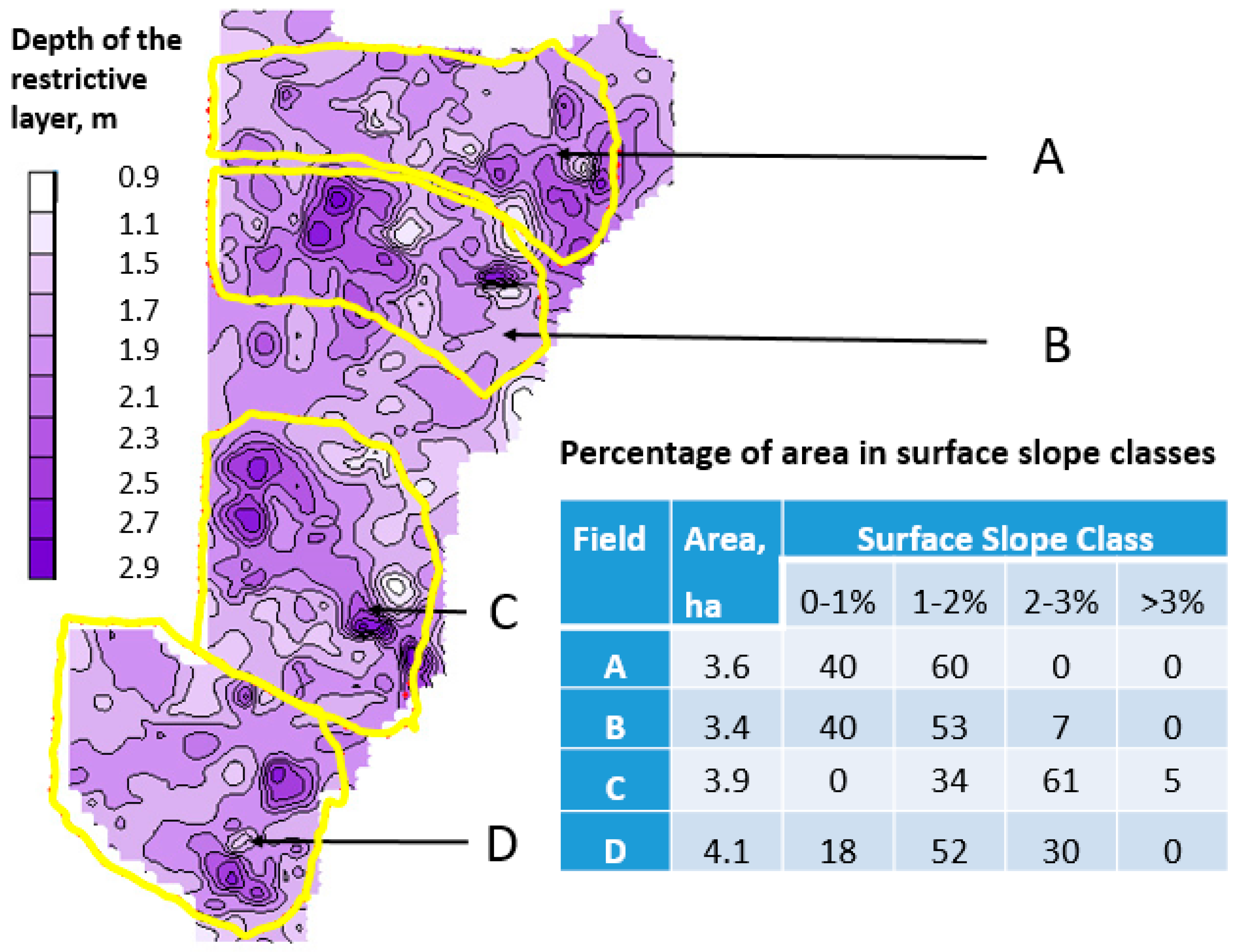
The Optimizing Production Inputs for Economic and Environmental Enhancement (OPE3) study site is located at the USDA-ARS Beltsville Agricultural Research Center, Beltsville, Maryland (near 39°01′44′′ N,76°50′46′′ W). The OPE3 site includes 21-ha of arable land which is subdivided into small hydrologically bounded fields surrounded by earthen berms. Fields A, B, C, and D ranged from 3.4 to 4.1 ha (Figure 1). The runoff from the fields feeds a wooded riparian wetland and first-order stream. The soils in the study site vary, but the dominant soils are coarse-loamy, mesic typic Hapludults. The surface soils in each field range from sandy loams to loamy sands [17]. Soil texture in the upper 0.3 m of these fields is nearly identical with the average sand content of 61 to 63% [18]. A continuous clay lens exists over the study field, with additional fractured lenses present intermittently [8,19]. These lenses form a restrictive layer for infiltration and facilitate the formation of perched shallow groundwater (Figure 1). The average depth of the restricting layers in each field is similar—about 1.5 m [18]. Surface slopes are slightly greater at field D than at fields A and B (Figure 1). Field C was excluded from the analysis in this work because its surface slopes and hydrologic response are very different from those at fields A, B, and D [20].
Planting dates and total N fertilizer applied are shown in Table 1. As recommended by the best management practices of the University of Maryland, 34 kg N/ha was applied in a band at planting as a starter fertilizer, and the balance was applied as side-dress at 4–5 weeks after planting. Field A received an application of bovine manure before planting, the starter fertilizer at planting, and a uniform side-dress applications of N fertilizer at 4–5 weeks after planting as determined by a pre-side-dress nitrate test (PSNT) because of N loss due to ammonia volatilization [21]. Field B received starter fertilizer at planting plus a uniform side-dress application of N fertilizer with the rate determined by the mean PSNT value. Field D received starter fertilizer at planting plus variable rate application of N fertilizer determined by subsurface hydrology and PSNT values in 2002 and 2004 [18]. After 2005, the N side-dress rate was determined by subsurface hydrology alone [18].
Daily precipitation was measured with a tipping bucket rain gauge near the edge of field B. Cumulative precipitation for 120 days was recorded starting 10 days before planting and ending at physiological maturity (Table 1). Corn grain yields were recorded with a harvester that had a yield monitor (Ag Leader 2000, Ames, IA, USA) interfaced with a differential GPS receiver. Mean corn grain yields for each field are shown in Table 1. Hurricane Isabelle in 2003 severely damaged the crop before harvest and yields are omitted. Data used in this work are available from the corresponding author upon request.
2.2. EOF Analysis
The Empirical Orthogonal Functions (EOF) analysis is a widely applied statistical method for analyzing large spatio-temporal datasets [22]. The idea of the method is to decompose the spatio-temporal changes of the studied variable into spatial patterns (EOFs) which are constant in time and time series (expansion coefficients, ECs) [23]. The decomposition equation is:
Here, Y is the measured value at the location s, at time t; is the average across all locations at time t. The original dataset can be reconstructed by the sum of products EOF and corresponding ECs. The first EOF (EOF1) explains the largest part of the variance of the differences Y(s,t) − , and subsequent EOFs explain progressively less variance. Only significant EOFs are selected. Expansion coefficients scale the contributions of EOFS to the deviations from the average for different years. EOFs have the same units as Y; ECs are unitless. In this study, EOF analysis was applied to characterize both the spatial and temporal variation of corn yields in fields A, B, and D separately to describe how nutrient management affected corn yields temporally and spatially. The eof.mca routine in R [24] was used to perform the EOF analysis. The semivariograms were used to analyze the spatial dependencies in EOFs among fields by establishing the degree of dissimilarity between observations as a function of the distance between observation points. The gstat package in R version 3.53 was used to compute semivariograms [25]. The cumulative distribution functions (CDFs) were constructed to compare EOFs from different fields. The Shapiro–Wilk statistics was used to compute probabilities of EOF2 being normally distributed.
2.3. The Restrictive Layer Topography and Subsurface Flow Pathways
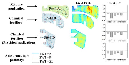
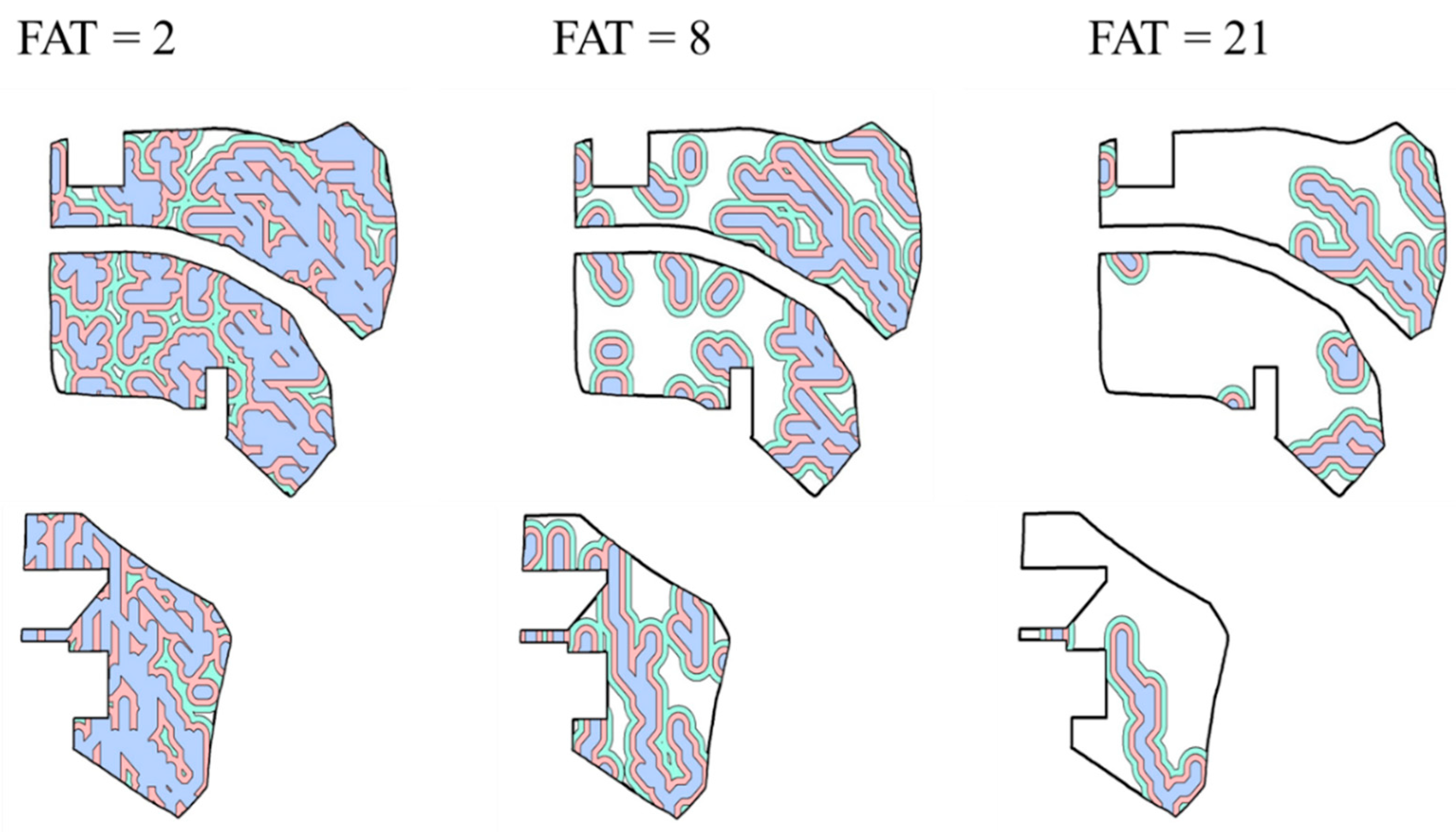
The stream delineation tool from the ArcMap hydrology toolset was applied to acquire the subsurface flow pathway network as described in Morgan et al., 2019 [26]. The kinematic GPS surveys and ground penetration radar survey provided the surface elevation and restrictive layer depths data, respectively [19]. The digital elevation model (DEM) of the subsurface restrictive layer was obtained by subtracting krigged depth of the restrictive layer. Then, the “flow direction” and “flow accumulation” tools in ArcGIS were used to determine potential subsurface flow pathways. The “flow direction” tool in ArcGIS was applied to the DEM of the restrictive layer to create a grid presenting the flow direction from each cell. The “flow accumulation” tool was applied to calculate accumulated water flow from its neighboring cells. Different flow accumulation thresholds (FATs) were applied to develop the subsurface flow pathway network which had a greater number of inflowing cells than thresholds. Each subsurface pathway network was changed to the feature layer by applying the “stream to feature” tool. Subsurface pathways for three FATs (2, 8, and 21) were calculated at fields A, B, and D [26]. Three buffer zones (0 to 5 m, 5 to 10 m, and 10 to 15 m) for each field were determined by the “buffer” function in ArcGIS, and the averages and the standard errors of EOFs across these zones were computed.
3. Results
3.1. EOF Analysis
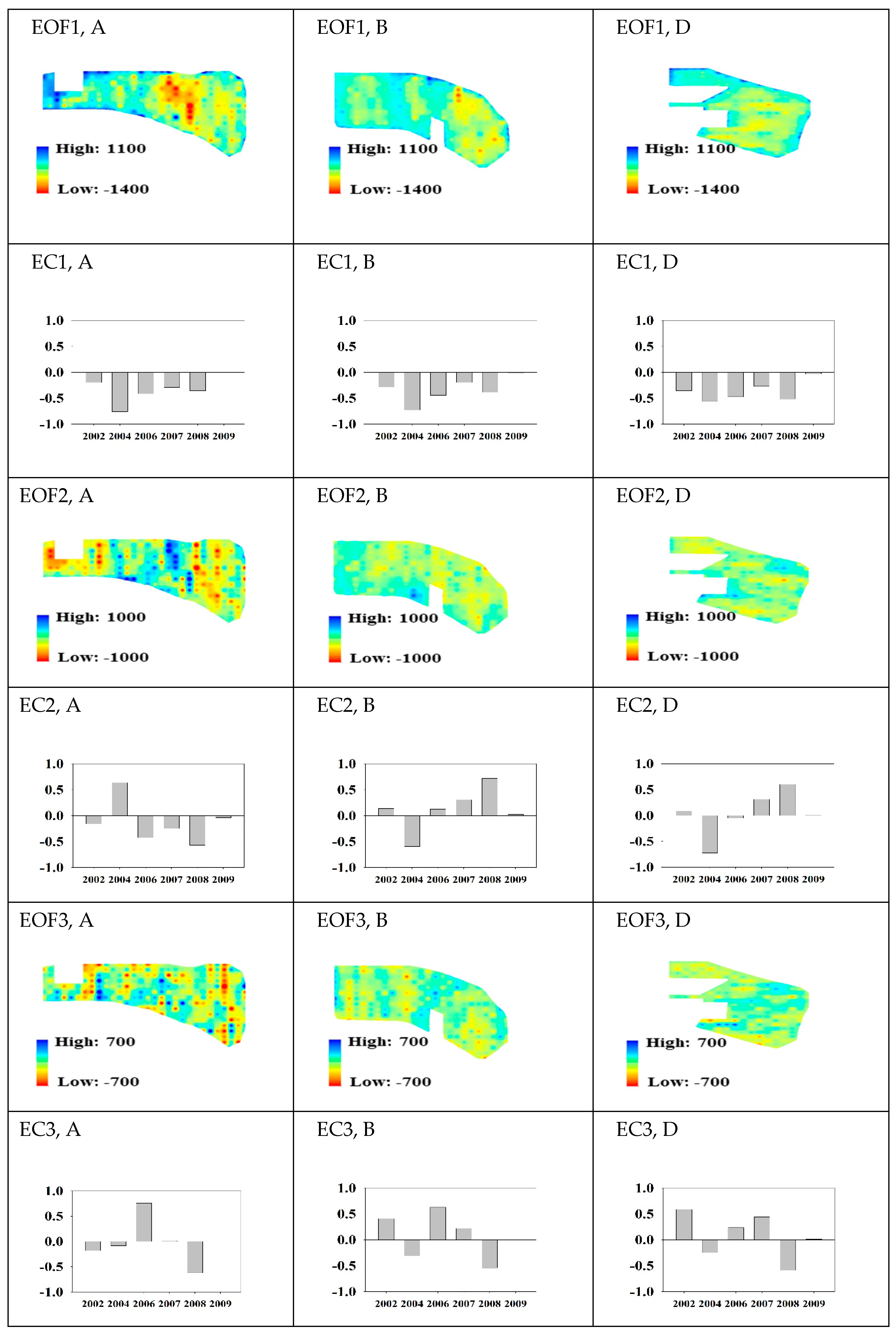
Figure 2 shows the three EOFs that explained the most spatial variation in corn yields in fields A, B, and D. The EOF1 explained 52.9, 52.0, and 56.5% of spatial variation; EOF2 explained 20.8, 17.9, and 17.9%; and EOF3 explained 11.1, 13.0, and 10.7% for fields A, B, and D, respectively. The EOF4 explained about 7% of variation at all fields. Ranges of EOF1 variation were much higher than ranges of variation of EOF2 and EOF3 at all three fields.
Contributions of EOFs to the deviations of the local yields from the average across the field ( are products of EOF and EC (Equation (1)). Therefore, the magnitude of the contributions is controlled by values of both EOF and EC. The higher the absolute value of an EC, the higher the contribution of the corresponding EOF. The shapes of the dependence of EC1 on time were similar for all three fields (Figure 2). For the years with spring planting days (2002–2007), the EOF1 contributions in wet high-yield years 2004 and 2006 were higher than in dry low-yield 2002 and 2007 years. In summer planting years 2008 and 2009, the contribution of the EOF1 was also higher in the wet high yield 2008. There was less variation in EC1 values among the observation years at field D as compared with fields A and B in the years with spring planting days. Signs of the EC2 values were opposite in field A compared with fields B and D (Figure 2) both in spring and in summer planting years. The absolute value of the EC2 was relatively high at field A in 2006 which was the year of the highest yield recorded in this field. Interannual contributions of EOF3 to values as defined by the absolute values of EC3 were relatively similar at fields B and D and very different from field A.
The cumulative distribution functions of EOF1, EOF2, and EOF3 are shown in Figure 3. Interestingly, CDF data sets of EOF1, EOF2, and EOF3 were similar across the fields. The distributions of EOF1, EOF2, and EOF3 in fields B and D were almost identical, whereas EOFs from field A had slightly larger variance. The Shapiro–Wilk test produced probabilities of EOF2 being normally distributed equal to 0.123, 0.453, and 0.544 for fields A, B, and D, respectively. The same test showed that the probability of the EOF1 being normally distributed was high only for field B (p = 0.475). EOF1 values across B and D were not normal (p < 0.0001), mostly because of heavy tails (Figure 3). The probabilities of distributions of EOF3 being normal were 0.165, 0.931, and 0.173 for fields A, B, and D, respectively. The ranges of EOF values, in general, decreased as the number of EOF increased.
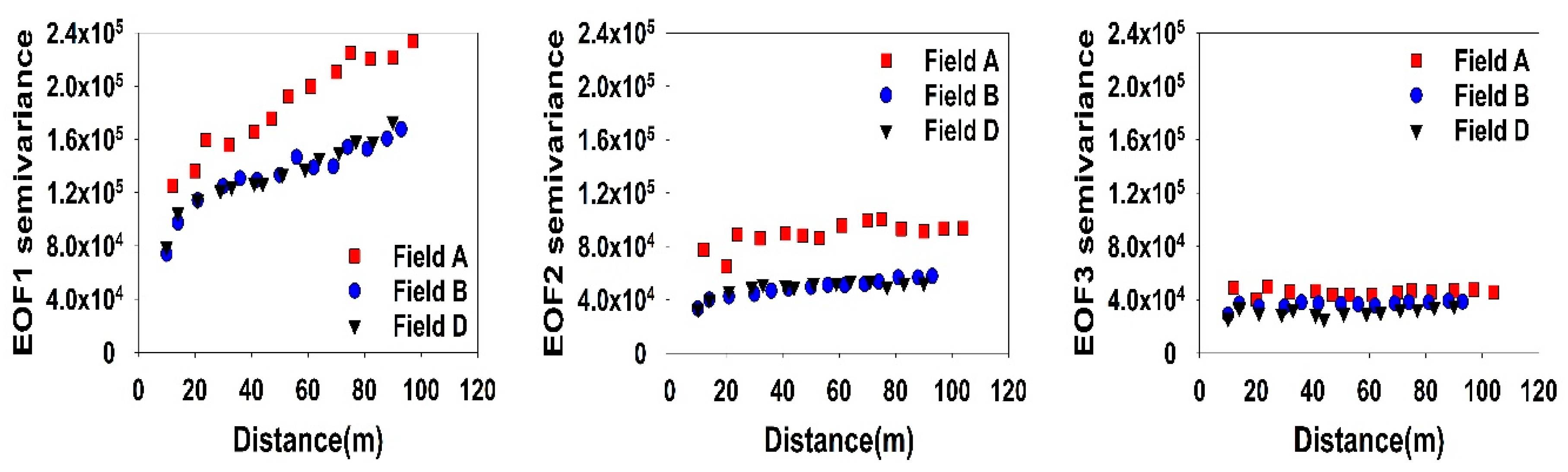
Semivariograms for each EOF from fields A, B, and D are shown in Figure 4. The EOF1 semivariogram for field A is distinctly different from that for fields B and D. The EOF1 semivariograms for both fields B and D demonstrate a clear spatial structure with the variance of the different observations increasing rapidly with the distance up to 40 to 50 m threshold value, and then slowly increasing. The EOF1 semivariogram for field A does not demonstrate a clear deceleration of the growth as the distance between observations increases. The EOF2 and EOF3 semivariograms for all fields do not show the clear spatial structure because their values of the semivariogram do not have the trend of growth with the distance.
The variance of EOF2 and EOF3 in fields B and D is 2 to 3 times lower than the variance of EOF1 across these fields. The semivariance of EOF1 is larger in field A as compared with fields B and D at every separation distance. The semivariogarms show that field A yield surface has higher roughness than fields B and D.
3.2. Subsurface Flow Pathways and EOFs
Buffer zones of three distance ranges (DR) from subsurface flow pathways are shown in Figure 5 for the three different flow accumulation thresholds (FAT).
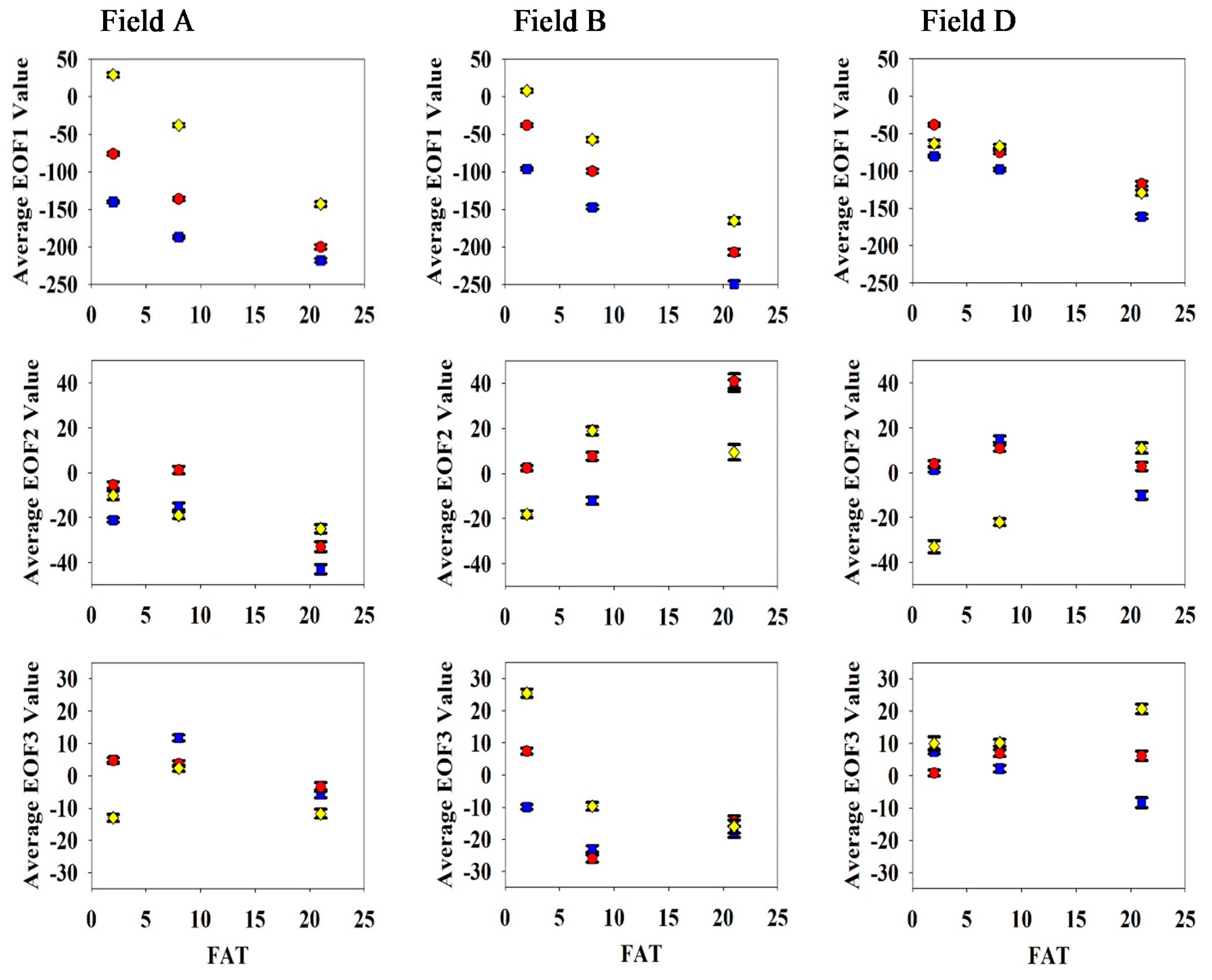
The average EOF values across the buffer zones are shown in Figure 6. The standard errors of EOFs across the zones varied between 0.7 and 4.4. They tended to be larger for EOF1 than for EOF2 and EOF3, and to increase with DR and FAT. For all FAT values, the increase in the DR led to the increase in the EOF1 value for all fields. One exception is field D where the average EOF1 for FAT = 2 and FAT = 8 at DR of 10–15 m was less than that at DR of 5 to 10 m. The sensitivity of the EOF1 to DR at field D was substantially lower than at fields A and B. The average EOF2 and EOF3 values were less sensitive to the DR value as compared to the average EOF1 values. The sensitivity of the EOF3 to DR at field D was slightly less than at fields A and B. Values of average EOF3 at FAT 21 at field D present the exception. Figure 6 shows that the average EOF3 values at field D varied slightly as the DR changed at FAT = 2 and FAT = 8, but showed a strong dependence on DR at FAT = 21.
4. Discussion
Local deviations of yields across fields from the average across the fields can be approximated as a sum of spatial patterns. The relative contribution of each pattern depends on the weather conditions of the specific year, and on the amount and type of fertilizer applied, and on spatial variation in the fertilizer doze. Areas of extreme values of EOF1 do not coincide with extreme values of EOF2 and EOF3, probably because the three EOFs reflect different factors that affected crop yields.
The EOF1 pattern explains most of the variability (52.0 to 56.5%) and appears to be related to the topography of the restrictive layer, which is relatively close to the soil surface and can control water dynamics in soil and corn root zone [19]. The argument in favor of that assumption is that this pattern is sensitive to the distance to the subsurface flow pathways (Figure 6). Another argument is that in years of spring planting 2002–2007, the expansion coefficients EC1 were higher in high yielding 2004 and 2006 compared with low-yield 2002 and 2007 that had a relatively low cumulative precipitation during the vegetative period (CPDVP). Subsurface flow probably was more active during years with high CPDVP, and the distance to the flow pathways could be more influential compared with the low CPDVP conditions. The differences in signs of EC2 among the fields and similarity of interannual differences between B and D indicate the possibility of EC2 being at least partially controlled by the type of fertilizer. The maximum difference in values of EC2 between A and B and A and D could arise from the differences in the release, mobility, and availability in fertilizer nutrients under high CPDVP conditions. Larger leaching of nitrogen from the soil root zone has been noted for chemical fertilizer compared with manure application (e.g, [27]). The difference in the fertilizer type could be the reason for the cardinal differences between EC3 in fields A and B and similarity of EC3 in fields B and D. The similarity in EC values between fields B and D indicates that the subtle difference between the distribution of slope classes shown in Figure 1 does not strongly affect the relative role of spatial patterns EOF1, EOF2, and EOF3 in local deviations of yields from the average yield across the fields. We realize that the CPDVP is a very imprecise metric of the effect of water availability on yields during the vegetative period. Observations made in this work do not consider the influence of intra-annual precipitation dynamics on yields at the study fields. Dependencies of EC2 and EC3 on time may reflect differences in nutrient management, surface slope, and field geometry. Coarse-textured soils of the study site could develop some degree of hydrophobicity and water repellency after a multiyear manure application [28,29,30]. No data were available to distinguish the effects of the aforementioned water availability factors.
The spatial correlation structure of the EOF1 pattern was different between the fields receiving chemical fertilizer (fields B and D) and manure (field A). While the fields with chemical fertilizer had semivariograms of classic shapes with the sill and the range, the manured field had the additional heterogeneity added with scale increase and the semivariogram looked like a power-law one (Figure 4). A possible explanation is that while the chemical fertilizer is homogeneous in terms of nutrient content, manure is not. The accumulation of the manure before the application continued for three to four months, and different parts of the field received manure that spent different times in storage and could have different fertilizer content. This might also be reflected in different variability of EOF1 across the field visible in Figure 2.
The ArcGIS routine localizes the potential subsurface flow pathways but cannot provide the actual amount of water flowing through these pathways. Using different FAT also does not provide water volumes but provides information about the complexity of the network. Larger FAT values lead to creating more complex networks of potential flow paths. Adding the complexity allows one to obtain more evidence on the effect of the proximity to the subsurface flow pathway on the deviation of local yield from the field averaged value.
Precision N applications in field D were adjusted for subsurface hydrology (flow patterns) that provided water and nutrients to the crop root zone [18]. The results of this adjustment are reflected in Figure 6 where the distance from the pathways affects the pattern EOF1 at the field D slightly for all considered FAT values. This leads to a substantial decrease in yield spatial variability. If EOF1 quantifies soil water-related variability, then the precision application of nutrients appears to implicitly account for this variability and mitigate it.
5. Conclusions
This study investigated the spatial and temporal patterns of corn yields as affected by subsurface preferential lateral flow pathways and different nutrient management practices. Data from six years of yield monitoring were analyzed. The deviations of yields from average values were expressed as sums of weighted spatial patterns (EOFs). The spatial patterns did not change with time, but their weights did. The first pattern was most probably associated with the topography of the subsurface pathways and explained about 52 to 56% of the interannual yield variability. The second and third patterns explained much less variability and could not be explicitly associated with subsurface topography. Spatial variability in EOFs as characterized by semivariograms and was more pronounced at the manured field as compared with the fields with the chemical fertilizer application. The dependence of the yields on the topography of the subsurface restrictive layer was to the large extent mitigated by the precision applications of nitrogen fertilizer. Establishing spatial patterns of yield variability for this type of agronomic control continues to present a promising research avenue to explore.
Author Contributions
Conceptualization, Y.P.; Data curation, C.D. and A.R.; Formal analysis, S.K.; Investigation, A.P.-P.; Methodology, S.K. and Y.P.; Resources, Y.P.; Supervision, Y.P.; Writing—original draft, S.K.; Writing—review and editing, C.D., A.R., A.P.-P. and Y.P. All authors have read and agreed to the published version of the manuscript.
Funding
This research received no external funding
Conflicts of Interest
The authors declare no conflict of interest.
References
- Daughtry, C.S.T.; Gish, T.J.; Dulaney, W.P.; Walthall, C.L.; Kung, K.J.; McCarty, G.W.; Angier, J.T.; Buss, P. Surface and subsurface nitrate flow pathways on a field scale. Sci. World J. 2001, 1, 155–162. [Google Scholar] [CrossRef] [Green Version]
- Nawar, S.; Corstanje, R.; Halcro, G.; Mulla, D.; Mouazen, A.M. Delineation of soil management zones for variable-rate fertilization: A review. Adv. Agron. 2017, 143, 175–245. [Google Scholar]
- Reyes, J.; Wendroth, O.; Matocha, C.; Zhu, J. Delineating Site-Specific Management Zones and Evaluating Soil Water Temporal Dynamics in a Farmer’s Field in Kentucky. Vadose Zone J. 2019, 18, 1. [Google Scholar] [CrossRef]
- Whetton, R.; Zhao, Y.; Mouazen, A.M. Quantifying individual and collective influences of soil properties on crop yield. Soil Res. 2018, 56, 19–27. [Google Scholar] [CrossRef] [Green Version]
- Kahlown, M.A.; Ashraf, M. Effect of shallow groundwater table on crop water requirements and crop yields. Agric. Water Manag. 2005, 76, 24–35. [Google Scholar] [CrossRef]
- Zipper, S.C.; Soylu, M.E.; Booth, E.G.; Loheide, S.P. Untangling the effects of shallow groundwater and soil texture as drivers of subfeld-scale yield variability. Water Resour. Res. 2015, 51, 6338–6358. [Google Scholar] [CrossRef] [Green Version]
- Yoder, R.E.; Freeland, R.S.; Ammons, J.T.; Leonard, L.L. Mapping agricultural fields with GPR and EMI to identify offsite movement of agrochemicals. J. Appl.Geophys. 2001, 47, 251–259. [Google Scholar] [CrossRef]
- Gish, T.J.; Dulaney, W.P.; Kung, K.J.; Daughtry, C.S.T.; Doolittle, J.A.; Miller, P.T. Evaluating use of ground penetrating radar for identifying subsurface flow pathways. Soil Sci. Soc. Am. J. 2002, 66, 1620–1629. [Google Scholar] [CrossRef] [Green Version]
- Tromp-van Meerveld, H.J.; McDonnell, J.J. Threshold relations in subsurface stormflow: 2. The fill and spill hypothesis. Water Resour. Res. 2006, 42, 2. [Google Scholar] [CrossRef] [Green Version]
- Vereecken, H.; Pachepsky, Y.; Simmer, C.; Rihani, J.; Kunoth, A.; Korres, W.; Shao, Y. On the role of patterns in understanding the functioning of soil-vegetation-atmosphere systems. J. Hydrol. 2016, 542, 63–86. [Google Scholar] [CrossRef]
- Navarra, A.; Simoncini, V. A Guide to Empirical Orthogonal Functions for Climate Data Analysis; Springer Science & Business Media: New York, MY, USA, 2010; pp. 39–67. [Google Scholar]
- Martinson, D.G. Quantitative Methods of Data Analysis for the Physical Sciences and Engineering; Cambridge University Press: Cambridge, UK, 2018. [Google Scholar]
- Cantelaube, P.; Terres, J.; Doblas-Reyes, F.J. Influence of climate variability on european agriculture—Analysis of winter wheat production. Clim. Res. 2004, 27, 135–144. [Google Scholar] [CrossRef]
- Rodríguez-Puebla, C.; Ayuso, S.M.; Frías, M.D.; García-Casado, L.A. Effects of climate variation on winter cereal production in Spain. Clim. Res. 2007, 34, 223–232. [Google Scholar] [CrossRef] [Green Version]
- Chun, J.A.; Kim, S.; Lee, W.; Oh, S.M.; Lee, H. Assessment of multimodel ensemble seasonal hindcasts for satellite-based rice yield prediction. J. Agric. Meteorol. 2016, 72, 107–115. [Google Scholar] [CrossRef] [Green Version]
- Cordero, E.; Longchamps, L.; Khosla, R.; Sacco, D. Spatial management strategies for nitrogen in maize production based on soil and crop data. Sci. Total Environ. 2019, 697, 133854. [Google Scholar] [CrossRef] [PubMed]
- Gish, T.J.; Dulaney, W.P.; Daughtry, C.S.T.; Kung, K.J.S. Influence of preferential flow on surface runoff fluxes. In Proceedings of the ASAE International Symposium of Preferential Flow, Honolulu, HI, USA, 3–5 January 2001; pp. 205–209. [Google Scholar]
- Gish, T.J.; Daughtry, C.S.T.; Russ, A.; McKee, L.; Prueger, J. Improved nitrogen management utilizing ground-penetrating radar: A nine-year investigation. In Proceedings of the 4th Interagency Conference on Research in the Watersheds, Fairbanks, AK, USA, 26–30 September 2011; pp. 94–99. [Google Scholar]
- Gish, T.J.; Walthall, C.L.; Daughtry, C.S.T.; Kung, K.S. Landscape and field processes: Using soil moisture and spatial yield patterns to identify subsurface flow pathways. J. Environ. Qual. 2005, 34, 274–286. [Google Scholar] [CrossRef] [PubMed]
- Gish, T.J.; Dulaney, W.P.; Daughtry, C.S.T.; Kung, K.-J.S. Influence of Preferential Flow on Surface Runoff Fluxes. 2008. Available online: https://hrsl.ba.ars.usda.gov/ope3/poster01.htm (accessed on 13 October 2020).
- Meisinger, J.J.; Bandel, V.A.; Angel, J.S.; O’Keefe, B.E.; Reynolds, C.M. Presidedress soil nitrate test evaluation in Maryland. Soil Sci. Soc. Am. J. 1992, 56, 1527–1532. [Google Scholar] [CrossRef]
- Jolliffe, I.T. Principal Component Analysis; Springer Series in Statistics: New York, NY, USA, 2002. [Google Scholar]
- Korres, W.; Koyama, C.N.; Fiener, P.; Schneider, K. Analysis of surface soil moisture patterns in agricultural landscapes using Empirical Orthogonal Functions. Hydrol. Earth Syst. Sci. 2010, 14, 751–764. [Google Scholar] [CrossRef] [Green Version]
- Available online: https://github.com/marchtaylor/sinkr (accessed on 7 July 2020).
- R Core Team. R: The R Project for Statistical Computing. 2019. Available online: http://www.R-project.org/ (accessed on 7 July 2020).
- Morgan, B.J.; Daughtry, C.S.; Russ, A.L.; Dulaney, W.P.; Gish, T.J.; Pachepsky, Y.A. Effect of shallow subsurface flow pathway networks on corn yield spatial variation under different weather and nutrient management. Int. Agrophys. 2019, 33, 271–276. [Google Scholar] [CrossRef]
- Yanan, T.; Emteryd, O.; Dianqing, L.; Grip, H. Effect of organic manure and chemical fertilizer on nitrogen uptake and nitrate leaching in a Eum-orthic anthrosols profile. Nutr. Cycl. AgroecoSyst. 1997, 48, 225–229. [Google Scholar] [CrossRef]
- Miller, J.J.; Beasley, B.W.; Hazendonk, P.; Drury, C.F.; Chanasyk, D.S. Influence of long-term application of feedlot manure amendments on water repellency of a clay loam soil. J. Environ. Qual. 2017, 46, 667–675. [Google Scholar] [CrossRef]
- Voelkner, A.; Diercks, C.; Horn, R. Compared impact of compost and digestate on priming effect and hydrophobicity of soils depending on textural composition. Die Bodenkult. J. Land Manag. Food Environ. 2019, 70, 47–57. [Google Scholar] [CrossRef] [Green Version]
- Wanniarachchi, D.; Cheema, M.; Thomas, R.; Kavanagh, V.; Galagedara, L. Impact of Soil Amendments on the Hydraulic Conductivity of Boreal Agricultural Podzols. Agriculture 2019, 9, 133. [Google Scholar] [CrossRef] [Green Version]
Figure 1.
Locations, depth of the restricting layer, m, and statistics of surface slopes at the OPE3 fields A, B, C, and D. Adapted from [20].
Figure 1.
Locations, depth of the restricting layer, m, and statistics of surface slopes at the OPE3 fields A, B, C, and D. Adapted from [20].

Figure 2.
Empirical orthogonal functions EOF1, EOF2, and EOF3 (maps) and the corresponding expansion coefficients EC1, EC2, and EC3 (bar graphs) for corn yields at fields A, B, D at the OPE3 site.
Figure 2.
Empirical orthogonal functions EOF1, EOF2, and EOF3 (maps) and the corresponding expansion coefficients EC1, EC2, and EC3 (bar graphs) for corn yields at fields A, B, D at the OPE3 site.

Figure 3.
Cumulative distribution functions of the empirical orthogonal functions; ![Water 12 03339 i001]() field A,
field A, ![Water 12 03339 i002]() field B,
field B, ![Water 12 03339 i003]() field D.
field D.
 field A,
  field B,
  field D.
Figure 3.
Cumulative distribution functions of the empirical orthogonal functions; ![Water 12 03339 i001]() field A,
field A, ![Water 12 03339 i002]() field B,
field B, ![Water 12 03339 i003]() field D.
field D.
field A, field B, field D.
Figure 4.
Semivariograms of empirical orthogonal functions EOF1, EOF2, and EOF3 of the corn yields.

Figure 5.
Buffer zones 0–5 m ![Water 12 03339 i004]() , 5–10 m
, 5–10 m ![Water 12 03339 i005]() , and 10–15 m
, and 10–15 m ![Water 12 03339 i006]() around the potential subsurface flow pathways derived with three flow accumulation threshold (FAT) values at fields A, B, and D.
around the potential subsurface flow pathways derived with three flow accumulation threshold (FAT) values at fields A, B, and D.
 , 5–10 m
  , and 10–15 m
  around the potential subsurface flow pathways derived with three flow accumulation threshold (FAT) values at fields A, B, and D.
Figure 5.
Buffer zones 0–5 m ![Water 12 03339 i004]() , 5–10 m
, 5–10 m ![Water 12 03339 i005]() , and 10–15 m
, and 10–15 m ![Water 12 03339 i006]() around the potential subsurface flow pathways derived with three flow accumulation threshold (FAT) values at fields A, B, and D.
around the potential subsurface flow pathways derived with three flow accumulation threshold (FAT) values at fields A, B, and D.
, 5–10 m , and 10–15 m around the potential subsurface flow pathways derived with three flow accumulation threshold (FAT) values at fields A, B, and D.
Figure 6.
Effect of the flow accumulation threshold (FAT) on the average EOF values across buffer zones created with different distances from the hypothetical subsurface flow pathways: ![Water 12 03339 i007]() 0 to 5 m buffer,
0 to 5 m buffer, ![Water 12 03339 i008]() 5 to 10 m buffer,
5 to 10 m buffer, ![Water 12 03339 i009]() 10 to 15 m buffer.
10 to 15 m buffer.
 0 to 5 m buffer,
  5 to 10 m buffer,
  10 to 15 m buffer.
Figure 6.
Effect of the flow accumulation threshold (FAT) on the average EOF values across buffer zones created with different distances from the hypothetical subsurface flow pathways: ![Water 12 03339 i007]() 0 to 5 m buffer,
0 to 5 m buffer, ![Water 12 03339 i008]() 5 to 10 m buffer,
5 to 10 m buffer, ![Water 12 03339 i009]() 10 to 15 m buffer.
10 to 15 m buffer.
0 to 5 m buffer, 5 to 10 m buffer, 10 to 15 m buffer.

Table 1.
Precipitation, applied nitrogen, and corn yields.
| Year | Planting Date | Total N Applied, kg N ha−1 | Cumulative Precipitation, mm | Corn Grain Yield, kg ha−1 | ||||
|---|---|---|---|---|---|---|---|---|
| Field A | Field B | Field D | Field A | Field B | Field D | |||
| 2002 | 17 April | 73 | 103 | 80 | 275 | 4796 | 5259 | 6153 |
| 2004 | 18 May | 154 | 172 | 109 | 402 | 7775 | 7508 | 6346 |
| 2006 | 29 April | 161 | 164 | 121 | 388 | 8783 | 7710 | 7474 |
| 2007 | 5 May | 161 | 164 | 121 | 188 | 4578 | 3428 | 3571 |
| 2008 | 28 June | 161 | 164 | 121 | 287 | 8571 | 7763 | 7359 |
| 2009 | 4 July | 117 | 164 | 121 | 382 | 6166 | 6013 | 6105 |
Publisher’s Note: MDPI stays neutral with regard to jurisdictional claims in published maps and institutional affiliations. |
© 2020 by the authors. Licensee MDPI, Basel, Switzerland. This article is an open access article distributed under the terms and conditions of the Creative Commons Attribution (CC BY) license (http://creativecommons.org/licenses/by/4.0/).
Share and Cite
MDPI and ACS Style
Kim, S.; Daughtry, C.; Russ, A.; Pedrera-Parrilla, A.; Pachepsky, Y. Analysis of Spatiotemporal Variability of Corn Yields Using Empirical Orthogonal Functions. Water 2020, 12, 3339. https://doi.org/10.3390/w12123339
AMA Style
Kim S, Daughtry C, Russ A, Pedrera-Parrilla A, Pachepsky Y. Analysis of Spatiotemporal Variability of Corn Yields Using Empirical Orthogonal Functions. Water. 2020; 12(12):3339. https://doi.org/10.3390/w12123339
Chicago/Turabian StyleKim, Seongyun, Craig Daughtry, Andrew Russ, Aura Pedrera-Parrilla, and Yakov Pachepsky. 2020. "Analysis of Spatiotemporal Variability of Corn Yields Using Empirical Orthogonal Functions" Water 12, no. 12: 3339. https://doi.org/10.3390/w12123339
Note that from the first issue of 2016, this journal uses article numbers instead of page numbers. See further details here.