Investigating the Structure of a Coastal Karstic Aquifer through the Hydrogeological Characterization of Springs Using Geophysical Methods and Field Investigation, Gökova Bay, SW Turkey

Abstract

The electrical resistivity tomography method has been widely used in geophysics for many purposes such as determining geological structures, water movement, saltwater intrusion, and tectonic regime modeling. Karstic springs are important for water basin management since the karst systems are highly complex and vulnerable to exploitation and contamination. An accurate geophysical model of the subsurface is needed to reveal the spring structure. In this study, several karst springs in the Gökova Bay (SW, Turkey) were investigated to create a 3D subsurface model of the nearby karstic cavities utilizing electrical resistivity measurements. For this approach, 2D resistivity profiles were acquired and interpreted. Stratigraphically, colluvium, conglomerate, and dolomitic-limestone units were located in the field. The resistivity values of these formations were determined considering both the literature and field survey. Then, 2D profiles were interpolated to create a 3D resistivity model of the study area. Medium-large sized cavities were identified as well as their locations relative to the springs. The measured resistivities were also correlated with the corresponding geological units. The results were then used to construct a 3D model that aids to reveal the cavity geometry in the subsurface. Additionally, several faults are detected and their effect on the cavities is interpreted.

1. Introduction

Geophysical surveys, especially electrical resistivity tomography (ERT) or its combination with induced polarization (IP) have been widely used in subsurface research for many years [1,2,3,4,5,6,7,8,9,10,11,12,13,14,15,16,17,18]. These nondirect methods are commonly applied on the surface or into boreholes for collecting information about the subsurface rock properties. These geophysical measurements can be interpreted in 2D, 3D, or 4D (time-lapse). These methods are also used in determining karstic structures, recharge, and discharge dynamics [19,20,21,22,23,24,25,26].

Karstic springs are the discharge points of karstic aquifers. These kinds of springs are of great importance in understanding karst systems. Modeling a karstic aquifer and its springs can contribute to enhance management and protection policies for the ecosystem in the studied watershed. Modeling can also provide accurate results on the ecological and hydrogeological evaluation of the region. Therefore, especially in recent years, scientists have been modeling river waters in terms of both flow and physicochemical properties [27,28,29,30,31,32,33]. These studies are also beneficial for flood risks and contamination issues both in the subsurface (vadose zone) and groundwater (saturated zone).

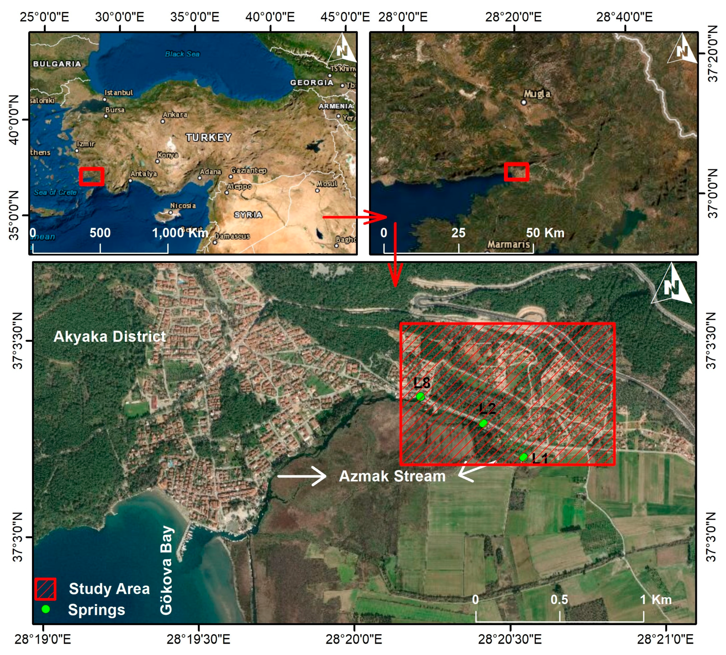
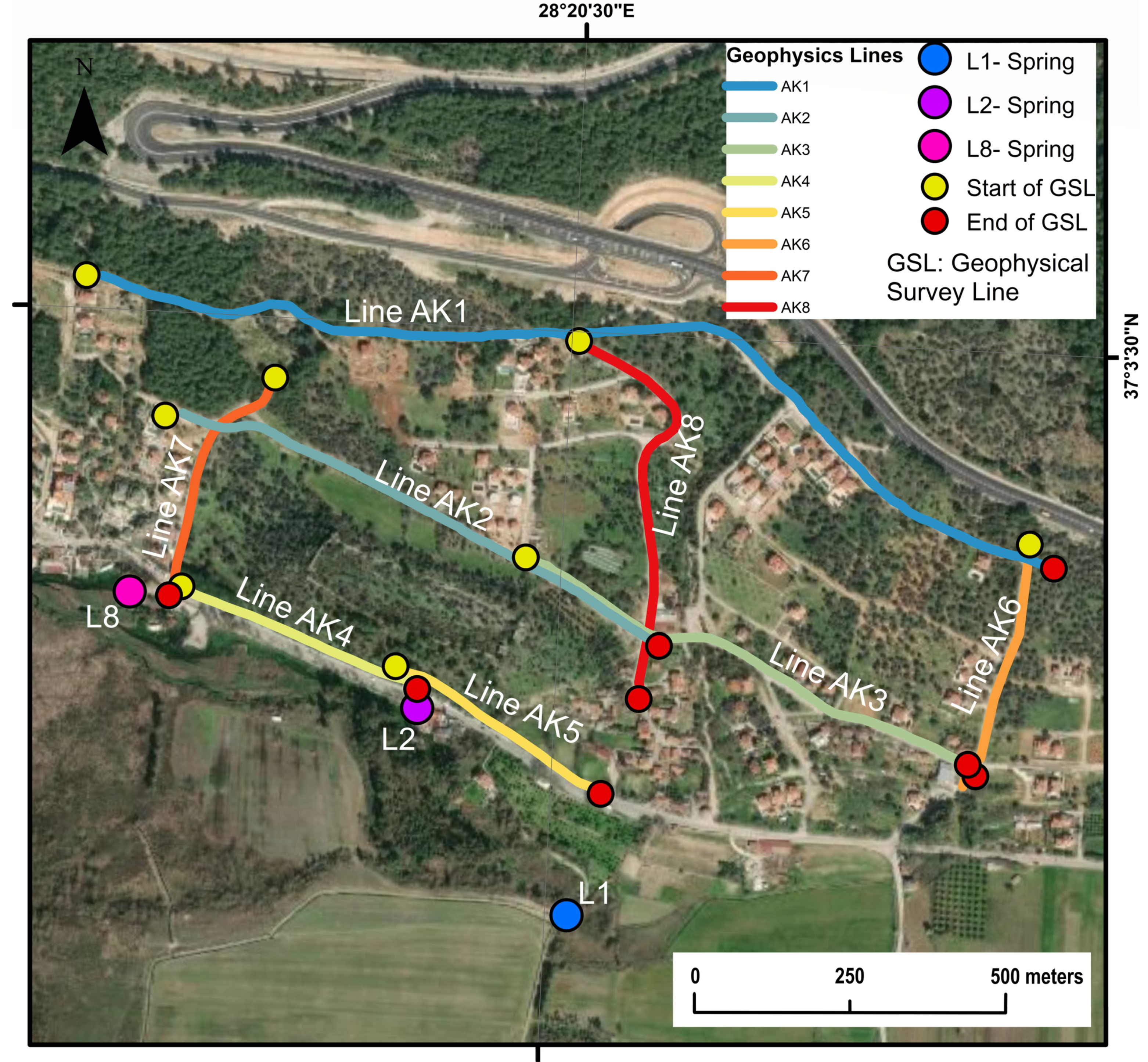
In this study, the Azmak Springs are examined, which are located Akyaka District (Ula, Muğla), Gökova Bay, the southwest coast of Turkey (Figure 1). There are around 40 large and small springs in the region. In addition, the Azmak Springs outflow into a 2 km long stream named Azmak as well. The Azmak Stream discharges to Gökova Bay. There are also submarine water sources in Gökova Bay [34,35,36]. These springs are known to be the discharge points of a large karstic aquifer that is widely extended in the region [37,38,39,40]. The electrical conductivity and flow rate of the spring water increase and decrease together. Thus, the salinization mechanism can be due to the venturi effect in such karst springs near the sea [37]. Several geophysical studies have been carried out in the alluvial plain of Gökova Bay. It was determined that the thickness of the alluvium unit containing clay lenses was 50 m towards the north near the springs and 160 m in the center of the plain [41,42,43,44,45]. Yet, the Azmak Springs have not been studied in terms of geophysics.

The Azmak Stream creates a wetland in the region, very close to the sea. Both Gökova Bay (sea) as well as the land, were designated as a special environmental protection area by the Turkish Ministry of Environment and Forests in 1988. Gökova Bay, the Azmak Stream, and the wetland host important fauna and flora such as otter (Lutra lutra), sand shark (Carcharinus plumbeus), island gull (Larus audoinii), Mediterranean monk seal (Monachus monachus), crested cormorant (Phalacrocorax aristotelis), red pine (Pinus brutia), oriental sweetgum (Liquidambar orientalis). Moreover, it should be noted that the Azmak Stream is a great tourist destination in the region that makes water management more difficult since the water consumption triples during the high tourist season. Over pumping to cover increasing water demand results in salinization by the sea-water intrusion.

Gökova Bay horst-graben structure is a product of tectonism that creates a major widening zone and affects all of western Turkey [46]. This horst-graben is structurally determinant on the karst aquifer in the region. The faults formed because of this tectonism are physically and chemically effective on the Azmak Springs. The relationship between the underground cavities of the Azmak Springs and local faults has not been studied before.

The physicochemical properties of the spring water are vital elements of the regional ecosystem [47,48,49]. For this reason, the underground physical structure of the Azmak Springs feeding the Azmak River, and the effects of the faults that are determinant in the formation of these springs have been investigated here using the geophysical electrical resistivity tomography method that has already proven its effectiveness in such studies [50,51,52].

2. Local Geology and Spring Water

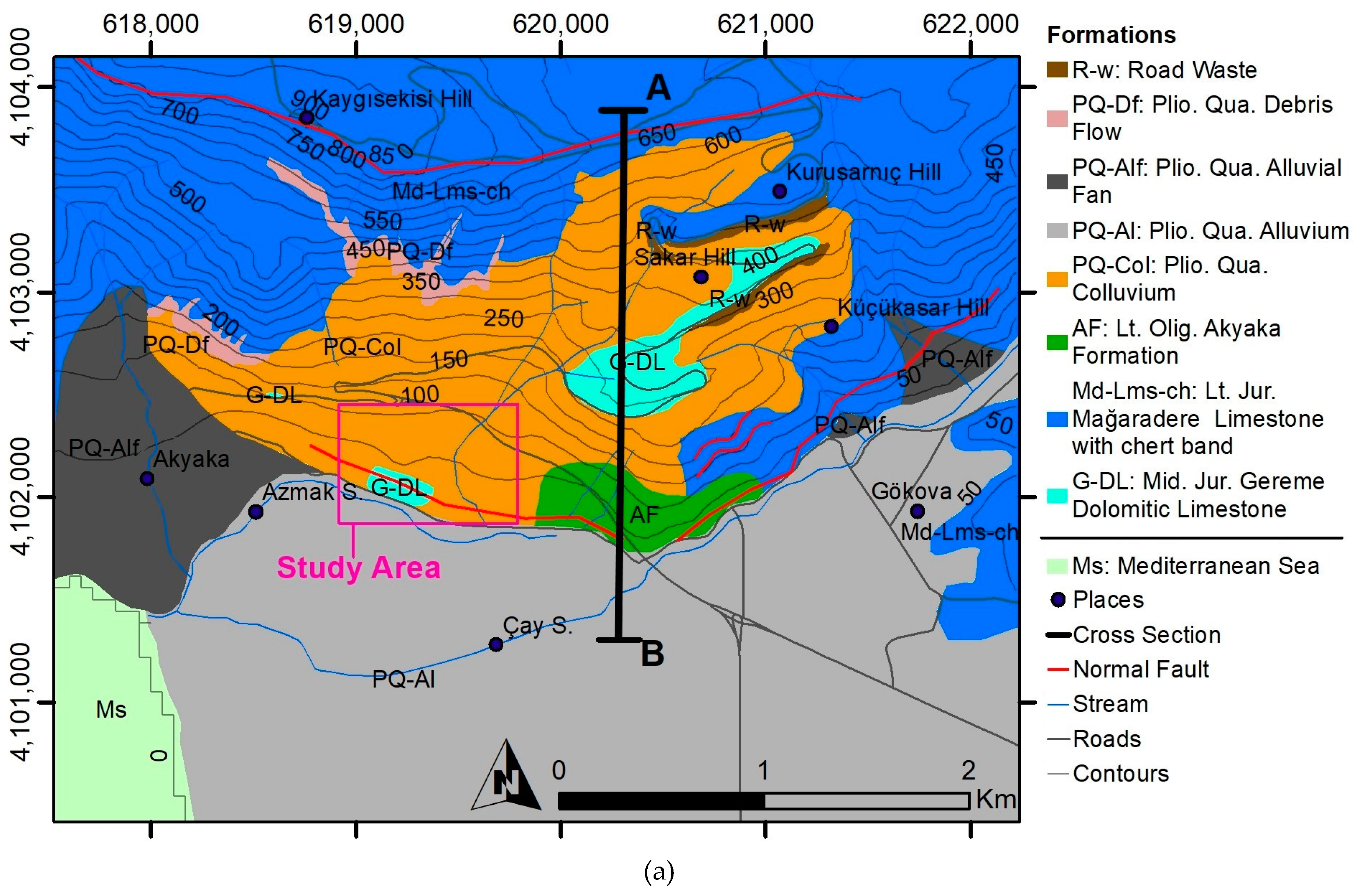
Gürer et al. [46] have studied the regional geology. They stated that Akyaka Formation consists of fossiliferous limestone on the top and grey-beige colored fluvial-alluvial conglomerate on the bottom. There is no Gökova alluvium at the horst-foot and there are colluvium, conglomerate, and limestone from top to bottom, stratigraphically. The basement rock consists of the Lycian nappes marble which belongs to the Late Cenozoic-Proterozoic age. These marbles are unconformably overlain by the Akyaka Formation (upper Oligocene age). Akyaka Formation continues through the west, crossing the geophysical study area, and uncomfortably covered by the Pliocene-Quaternary colluvium [46] (Figure 2).

Akyaka District, the Azmak Stream, and the Azmak Springs are located on the fault zone creating the horst and graben. The graben named Gökova Plain is covered by alluvium. In Akyaka District, the Azmak Springs have developed in the Late Triassic-Middle Jurassic aged Gereme Formation dolomitic-limestone unit. The dolomitic-limestone outcrop at the bottom of the horst. These karst springs recharge Azmak Stream in Akyaka District that discharges into Gökova Bay after a 2 km long surface flow.

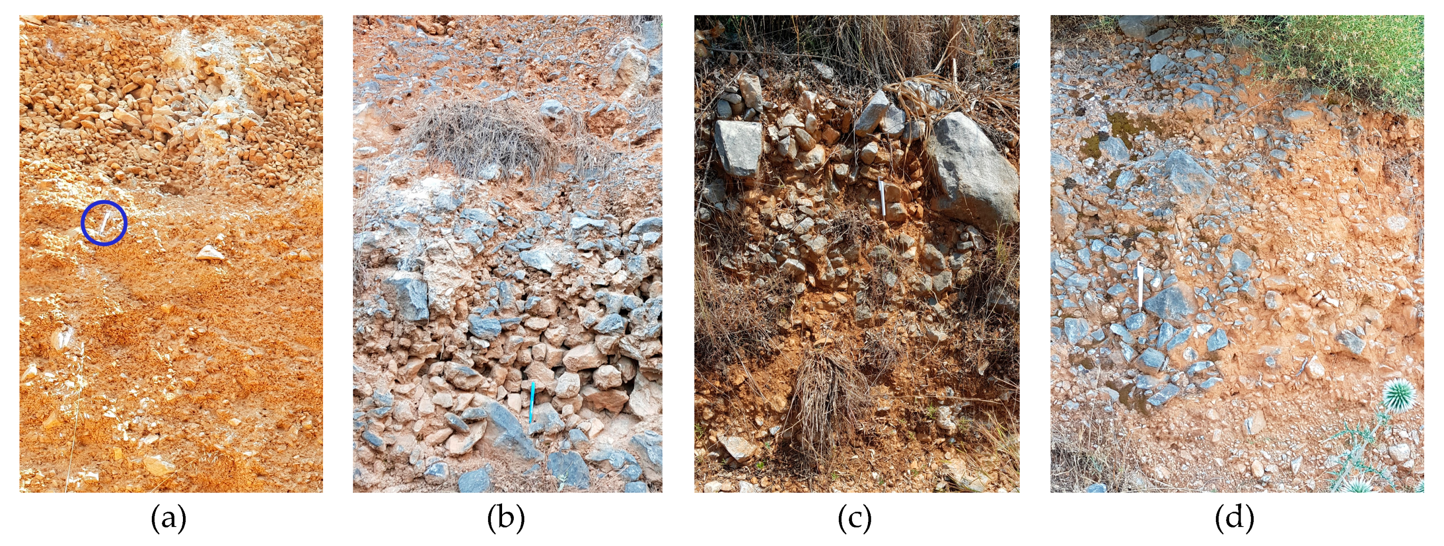
A one-week geological trip to the area was performed. Geological units and tectonic elements were investigated. Especially, the study area was examined in detail. Matrix-supported colluvium was the most encountered unit with variable grain size at the north of the geophysical survey area. Medium to large carbonate clasts are also found (Figure 3). These carbonate clasts comprise some voids in places that were created by surface runoff. These units are part of Plio-Quaternary Colluvium (PQ-Col).

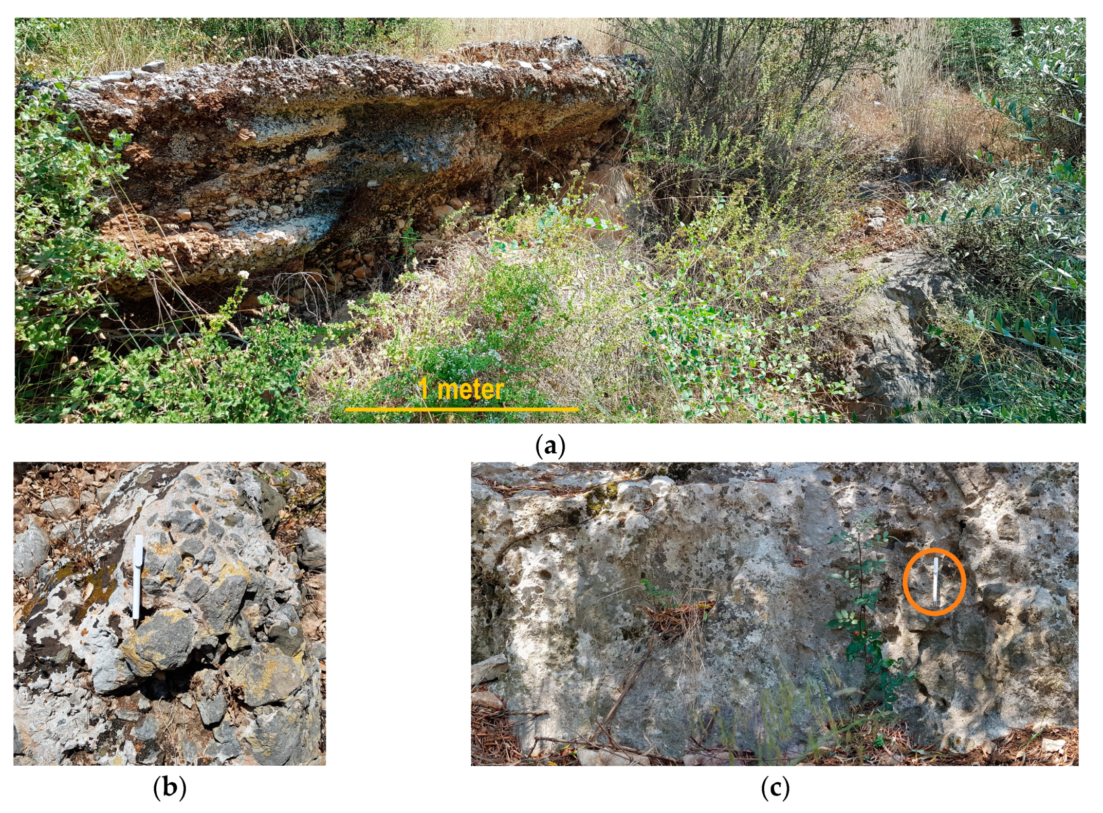
Middle Jurassic aged dolomitic-limestone blocks (Gereme Formation, G-DL) outcrop at the south of the area, alongside the stream (Figure 4a). Minor karst features were found in this unit. Additionally, from top to bottom stratigraphically, horizontally oriented colluvium, poorly rounded-sorted conglomerate, and dolomitic-limestone were located in the south. In the east of the area, soil, well-sorted poorly rounded matrix-supported colluvium (PQ-Col), medium-large dolomitic-limestone (G-DL) fragments were located from top to bottom, stratigraphically (Figure 4b). Barely well-rounded large rocks at this size were not very common at 70–80 cm depth in the north part of the study area.

In the west of the area, from top to bottom (stratigraphically), clast supported colluvium, conglomerate, and dolomitic-limestone were located on the site (Figure 5a). At the center of the area, from top to bottom (stratigraphically), poorly rounded conglomerate and dolomitic-limestone with minor karst feature (rill) were found (Figure 5b,c).

The tectonic elements of the study area play an important role in the formation of the springs and groundwater movement. Based on the field survey, a WWN-EES normal fault crosses the study area, along the Azmak Stream (Figure 2). The fault plane is visible on the dolomitic-limestone in the south of the area (Figure 4a).

The geophysical survey was conducted in August, which is the lowest flow period in the region. Flow rate, temperature, specific conductivity (at 25 °C), total dissolved solids, and salinity measurements of the spring waters were made every 15 days in the period of June, July, and August (

Table 1. Flow rate and some physicochemical values of the spring waters. Each value is the mean of measurements taken every 15 days in June, July, and August.

Springs	Flow Rate, Q (m3/h)	Temperature, T (°C)	Specific Conductivity, SpC (µS/cm)	Total Dissolved Solids, TDS (mg/L)	Salinity, Sal (mg/L)
L1	543	15.8	2050	1277	879
L2	141	16	3730	2013	1447
L8	860	15.5	3630	2079	1321

). The flow rate and physicochemical values of the water differ. Spring L1 is the farthest to the sea while the L8 is the nearest (Figure 1). Yet, neither the salinization nor the flow rate is ruled according to the distance to the sea. This phenomenon points out the complex subsurface cavity system. The most saline spring is L2 and it has the lowest flow rate and higher temperature. The seawater temperature was higher during the study period. The seawater intrusion is quite limited yet effective, considering the values of physicochemical parameters.

3. Materials and Methods

The ERT method was used to gather electrical resistivity values of the subsurface. The ERT survey was designed to characterize the local aquifer system and detect the fractures as they act as pathways for groundwater movement/discharge. Thus, based on the geological/tectonic settings of the study area, the ERT survey was designed. Then, the resistivity distribution of the subsurface was created and interpreted the geological, tectonic, and hydrogeological structures. In this study, subsurface cavities were investigated. These cavities are ending up with the springs and might have filled/semifilled by freshwater, seawater, or a mix of them. IP is a geophysical imaging method that is utilized to distinguish the electrical chargeability of the subsurface material [15,16]. IP measurements were taken during the deployment of ERT. IP was applied to assist the interpretation of the ERT results. The IP method is very sensitive to clay. Clay fillings were anticipated due to karstification in the survey area.

Both ERT and IP measurements were performed along eight lines using the multielectrode AGI Supersting R8 resistivity imaging system. ERT survey lines, AK1, AK2, AK3, AK4, and AK5, were conducted from West to East. The lines AK6, AK7, and AK8 were conducted from North to South (Figure 6). For the IP survey, maximizing the quality of the acquired data was attempted by optimizing the geometry of the IP survey, keeping at least one potential electrode in between the current electrode’s pair and maximize the collected signal [53]. Stainless steel electrodes instead of the recommended porous pot (Cu-CuSO₄) were used. The optimum injected current was selected, since it is proven that the more current is not always the best option [54]. An alternating polarity transmitter was used for the IP survey and hardware notch filter as well as stacking was applied to acquired data to minimize the noise [55]. The survey was performed in August which is the driest month in the region. The data acquisition was completed in five consecutive days to minimize the effect of seawater-groundwater level changes. The used array type in all measurements was Wenner-Schlumberger that offers the best vertical resolution and high sensitivity to lateral inhomogeneities [56]. Lateral resistivity changes were expected to be found based on local literature and other apriori information. The length of the lines, the number of electrodes, electrode spacing, depth of resistivity model, and the final root mean square errors (RMSE) after the inversions are given in

Table 2. Information about the geophysical survey lines.

Lines	Number of Electrodes	Electrode Spacing (m)	Line Length (m)	Depth of Resistivity Model (m)	Root Mean Square Error—RMSE (%)
AK1	56	20	1120	200–220	2.8
AK2 and AK3	56	10	560	100–120	3.1 and 2.9
AK4, AK5, AK6, and AK7	56	5	280	55–60	2.1, 4.2, 3.1, and 5.2
AK8	56	8	448	80–90	2.4

.

A differential GPS was used to locate each electrode for all the lines. The accurate coordinates of the electrodes were used during the inversion for applying the topographic correction.

The AGI EarthImager^TM 2D inversion modeling software was used for processing ERT and IP profiles. The finite difference method and the proper boundary conditions were used for forward modeling. For filtering the data, a low-pass filter with a moving average was applied. Damped least-squares, smooth model, and robust inversions were applied to the filtered data. The most reliable results based on the geology of the study area were constructed from the use of the damped least-squares inversion method. The iterative inversion procedure was terminated when the predefined RMSE limit (the difference between calculated and observed data) and the L2-norm statistics fulfill our convergence criteria. The average RMSE for ERT dataset, after the end of the inversion, was 3.23%. After processing the ERT and IP data, even most of the suggested ways were applied to improve the quality of the IP data as mentioned above. Yet, the quality of the IP data was found as not acceptable. Thus, IP data were not used for the interpretation.

After having the ERT sections, the geophysical survey area was revisited, and the outcropping units were located and identified. Then, it was determined which geological units in the field reflected which resistivity values, considering the consistency over the survey area. During the geophysical survey, several water wells were found. The depth to the groundwater level was measured and used for the validation of the geophysical sections.

The final data were imported in the RockWorks software to create a 3D subsurface geometry. In RockWorks, the anisotropic inverse distance weighting (IDW) method in the “Fence” module under “P-Data” in “Borehole Manager” was used to create a 3D model. Least-square optimization was applied for smoothing the interpolated data.

The final stage of the resistivity interpretation was to relate each resistivity range to the local geological unit. The outcropping geological units in the area were located and the corresponding electrical resistivities on the 2D ERT sections were determined. This is also part of the ground-truthing to produce the final geo-model from the 3D resistivity model of the study area. The resistivity values for some earth materials proposed by Palacky [57] are given

Table 3. Electrical resistivity of some earth materials proposed by [57].

Material	Resistivity (ohm-m)
Seawater	0.2–1
Fresh groundwater	3–100
Alluvium	10–1000
Limestone	>1000

. These were considered as base values and were used for comparison, not for interpretation.

4. Results

The average elevations around the northern, middle, and southern part of the study area were 100, 40, and 5 m above sea level (asl), respectively. The average geophysical investigation depths of the northern, middle, and southern part of the study area were 200, 100, and 50 m, respectively. Therefore, the average elevations of the bottom of the sections are 100, 50, and 50 m below sea level (bsl), respectively, from north to south. The Azmak Springs display a wide range of resistivity values between 5.6 and 10,000 ohm-m. These values show significant vertical and horizontal variations. The ERT sections are mostly composed of three layers. The resistivity values were investigated in three classes; lower resistivity zone between 0 and 400 ohm-m; medium resistivity zone between 400 and 1000 ohm-m; higher resistivity zone between 1000 and 10,000 ohm-m. The quite high resistivity values between 5000 and 10,000 ohm-m were found near the locations of the L2 and L8 springs. These high resistivity values are close to ground surface with an average of 30 m of vertical size. The general shape of these areas was averagely elliptic in lateral dimension. Additionally, some lateral changes in the resistivity values reflected the normal faults which are expected due to the hors-graben structure in the region.

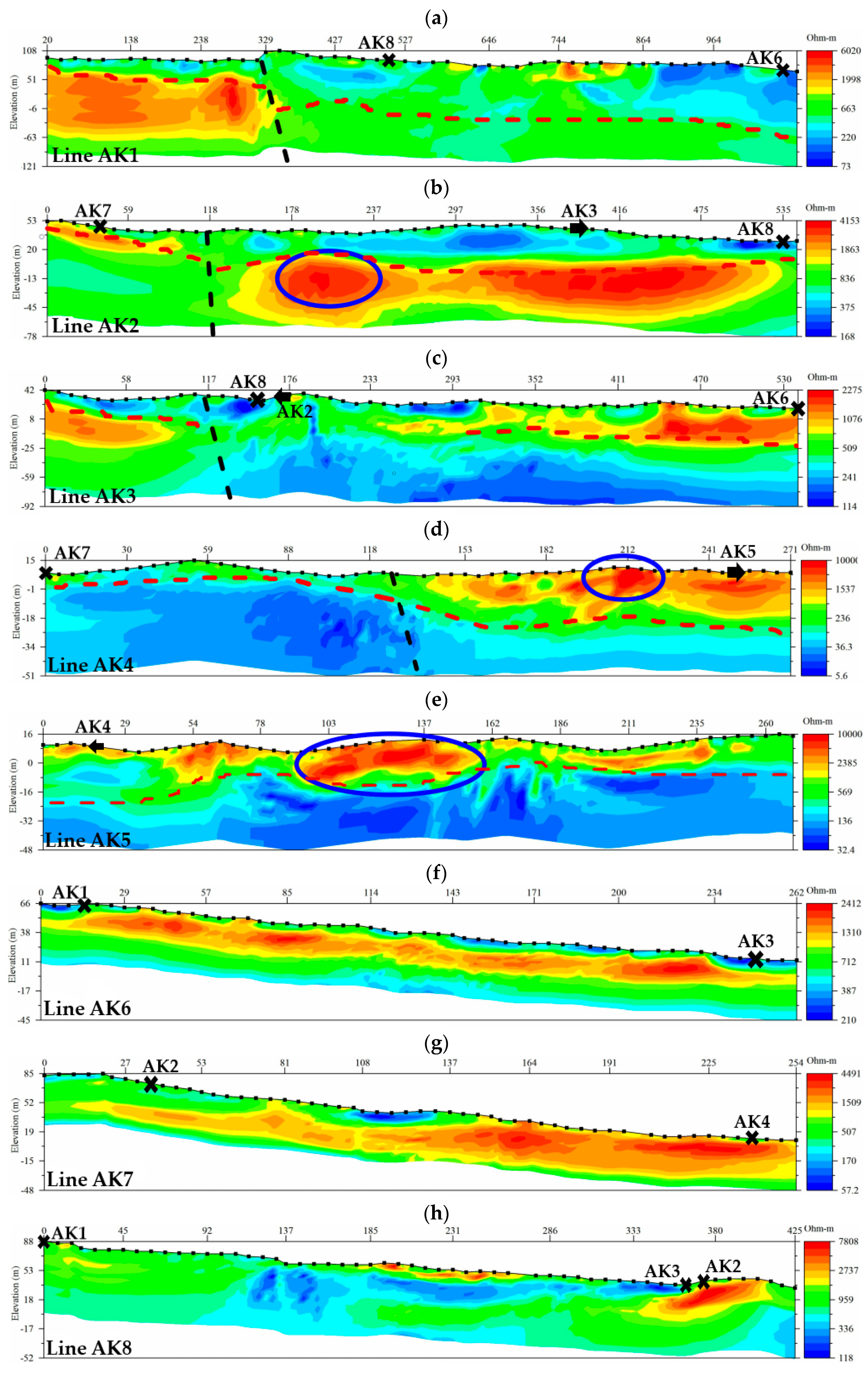
The line AK1 shows distinctive lateral change (Figure 7a). The zone with the resistivity values higher than 2000 ohm-m is located between 20 and 330 m along the line. Resistivity lower than 400 ohm-m is located between 880 m and the end of the line with 70–200 ohm-m. Other areas reflected 400–1000 ohm-m and 1000–2000 ohm-m resistivity values.

The line AK2 displays three main resistivity layers (Figure 7b). The first layer is represented by the values between 170 and 800 ohm-m and is located close to the surface roughly between 50 and 20 m elevation from the sea level. The second layer is represented by >2000 ohm-m and is located below the first layer. The resistivity value of the below layer is between 600 and 1000 ohm-m.

The line AK3 displays three main resistivity layers (Figure 7c). The first layer is represented by the values 100–500 ohm-m at between 10 and 40 m elevation from the sea level. The two zones with the resistivity values higher than 2000 ohm-m are under the first layer between 0 and 80 m with 35 m of thickness and between 300 and 560 m with 40 m of thickness. The third layer showed 500–750 ohm-m resistivity.

The line AK4 displays two main layers (Figure 7d). This section is mostly represented by low resistivity values, ranging between 0 and 700 ohm-m. The zone with over 2000 ohm-m extends from the center to the end of the line. The area between 80 and 120 m has the resistivity value of 5–35 ohm-m. Additionally, the blue circled area is notable with around 10,000 ohm-m resistivity at 210 m.

The line AK5 displays two main layers (Figure 7e). The top layer is around 10,000 ohm-m resistivity while the bottom is between 30 and 500 ohm-m. The blue circled area is notable with around 10,000 ohm-m resistivity between 100 and 150 m.

The line AK6 displays three main layers (Figure 7f). The resistivity of the top layer is between 210 and 800 ohm-m. The resistivity value of the middle layer is between 1300 and 2400 ohm-m while the bottom layer is changing from 200 to 800 ohm-m.

The line AK7 displays two main layers (Figure 7g). The resistivity of the top layer is between 50 and 700 ohm-m from 0 to 150 m along the line. The resistivity of the second layer is between 700 and 4500 ohm-m from 150 m to the end of the line.

The line AK8 displays three main lateral changes with two vertical layers (Figure 7h). The first layer with 600–1000 ohm-m is between 0 and 110 m along the line. The second layer with 118–600 ohm-m is between 110 and 340 m. The third layer with 2000–7800 ohm-m is from 340 m to the end of the line.

5. Discussion

5.1. Assessment of 2D ERT Sections

Several geological units were found in the geophysical survey area: matrix-supported colluvium (with voids in places), clast-supported colluvium, poorly rounded conglomerate, medium-large carbonate clasts, dolomitic-limestone blocks (with karst features in places).

The outcropped units were linked to the near-surface resistivity values. For the line AK1, the matrix-supported colluvium showed 400–800 ohm-m resistivity values while the large carbonate clasts gave 1200–200 ohm-m. For the line AK4, the dolomitic-limestone with minor karst features corresponded resistivity values higher than 4000 ohm-m. For the line AK5, the matrix-supported colluvium with voids and dolomitic-limestone gave 2800–4000 ohm-m and higher than 4000 ohm-m, respectively. For the line AK6, the matrix-supported colluvium reflected resistivity values between 1000 and 1400 ohm-m. For the line AK7, clast-supported colluvium, conglomerate, and dolomitic-limestone showed the resistivity values 1600–2400 ohm-m, 2400–4000 ohm-m, and higher than 4000 ohm-m, respectively. For the AK8 line, conglomerate and dolomitic-limestone with minor karst features corresponded 2000–4000 ohm-m and higher than 4000 ohm-m resistivity values, respectively. Overall, the geological units and the corresponding electrical resistivity values in the survey area are given in

Table 4. The proposed electrical resistivity values corresponding to the geological units in the survey area.

Material	Electrical Resistivity (ohm-m)
Matrix-supported colluvium	400–1400
Matrix-supported colluvium with voids	2800–4000
Clast-supported colluvium	1600–2400
Poorly rounded conglomerate	2000–4000
Medium-large carbonate clasts	1200–2000
Dolomitic-limestone	>4000
Dolomitic-limestone with minor karst features	>4000

.

Based on the electrical resistivity values of the outcropping geological units and the geological background of the survey area, 2D ERT sections were interpreted. It should be mentioned that concerning the karstic conduit modeling and interpretation using the ERT, the interpretation is mainly quantitative due to the limitation of the ERT related to electrode spacing and n-level measured resolution.

It was observed that some resistivity values do not exactly match each other at the crossing points of the geophysical lines. Along a depth ranging from 0 to −50 m asl, at the crossing between the AK4 and AK7, AK4 section showed around 20 ohm-m while AK7 section showed around 500 ohm-m. Although this is quite rare, this may be due to the higher error margin at the edges of the sections considering that the crossing of the AK4-AK7 is located at the edge of the section.

For the line AK1, the area between 20 and 330 m along the line is interpreted as dolomitic-limestone (Figure 7a). The thickness of dolomitic-limestone is around 100 m and it is under the colluvium unit. The resistivity values higher than 10,000 ohm-m might be the indication of the cavities [58,59]. The area located between 880 m and the end of the line is considered as fully saturated formations and is interpreted as two different units; clay-rich matrix-supported colluvium with 70–200 ohm-m resistivity and carbonate clasts with 200 and 400 ohm-m resistivity values. The black dashes at 310, 620, and 860 m are interpreted as faults, due to lateral changes of resistivity. Other units in 400–1000 ohm-m are interpreted as unsaturated colluvium. The areas between 1000 and 2000 ohm-m are interpreted as dolomitic-limestone. The reason is that these units are most probably filled with fine-grained units.

For the line AK2, the upper layer (170–800 ohm-m) and the middle layer (>2000 ohm-m) are interpreted as colluvium and dolomitic-limestone, respectively (Figure 7b). The third (bottom) layer is the carbonate clasts. In addition, the dashes at 118 and 260 m are defined as faults. The weak zone around the fault at 260 m is distinct.

For the line AK3, the zone with the resistivity values higher than 2000 ohm-m is between 0 and 80 m along the line with 35 m of thickness and between 300 and 560 m with 40 m of thickness are interpreted as dolomitic-limestone (Figure 7c). The dolomitic-limestone outcrops after 300 m. The second layer consists of colluvium and carbonate clasts (400–750 ohm-m). The black dashes at 110 and 280 m are interpreted as faults. Faulting in this area created the lower resistivity zone.

For the line AK4, the zone with over 2000 ohm-m resistivity that extends from the center to the end of the profile is interpreted as dolomitic-limestone of a thickness between 25 and 30 m (Figure 7d). This part matches up with the L2 spring location. The red circled area between 80 and 120 m showed 5–35 ohm-m resistivity value which is probably due to the seawater intrusion through the springs. The blue circled area with around 10,000 ohm-m resistivity at 210 m with 8–12 m of thickness is interpreted as a karst cavity.

For the line AK5, the top layer around 10,000 ohm-m resistivity is also interpreted as a karst cavity in dolomitic-limestone (Figure 7e). This part up to 160 m along the line also matches up with the L2 spring location as it is the same case for the AK4. The bottom layer is probably highly fractured dolomitic-limestone which contains brackish water.

For the line AK6, the top layer is composed of colluvium and carbonate clasts (210–900 ohm-m) (Figure 7f). The thickness of this unit varies between 2 and 15 m. The middle layer is interpreted as highly fractured dolomitic-limestone with fresh-water content (>1000 ohm-m) of a thickness ranging from 25 to 30 m. The bottom layer is composed of colluvium (400–1000 ohm-m).

For the line AK7, the top layer from 0 to 150 m along the line is interpreted as colluvium (Figure 7g). The thickness of this unit is changing from 15 to 35 m. As the second layer, dolomitic-limestone outcrops after 160 m along the line, near the Azmak Stream. The thickness of the dolomitic-limestone varies between 40 and 50 m. The dolomitic-limestone unit continues to the beginning of the profile in a highly fractured form under the colluvium. L8 spring was developed in this unit.

For the line AK8, from the beginning to 120 m along the line is interpreted as colluvium (Figure 7h). The blue zone at 135 m is evaluated as a fault zone. The resistivity of the area between 110 and 300 m matches the typical groundwater resistivity (Table 3) [57]. The underground cavity for the L1 spring in this section can be seen at 380 m. This unit between 350 and 400 m is dolomitic-limestone containing minor cavities with over 5000 ohm-m resistivity.

5.2. 3D ERT Model

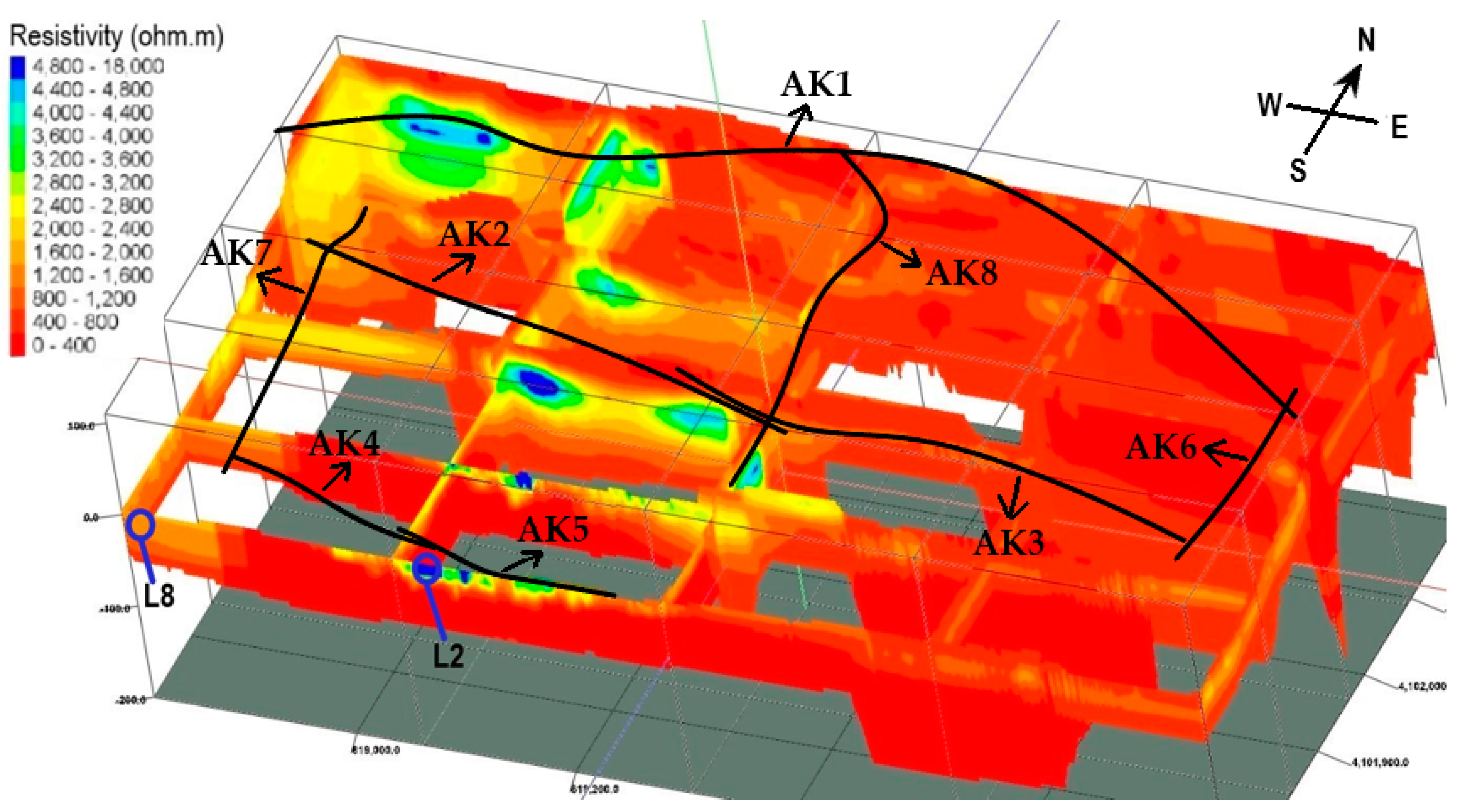
The 3D model was illustrated by limiting the values according to resistivity levels to understand the geometry and to assess the lithology and hydrogeology of the study area. The survey lines are not visible on the model. The model is visually manipulated to show the zones of interest. The 3D resistivity model of the studied region is shown in Figure 8, by using the fence representation. The area with the resistivity higher than 4000 ohm-m, clearly reveals the karstic network which makes it easier to see the continuity of the cavity geometry of the L8 and L2 springs.

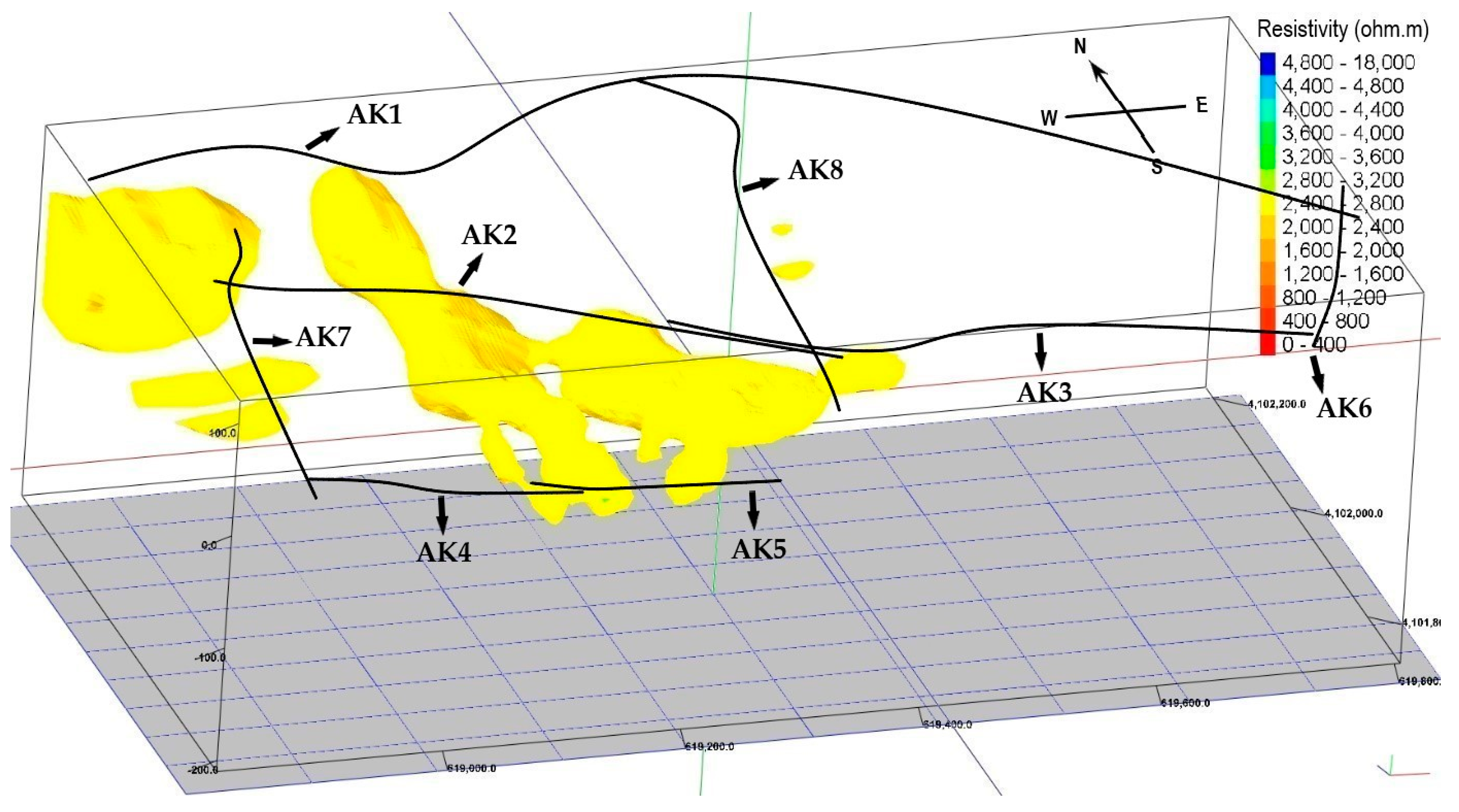
The areas greater than 2000 and 1000 ohm-m are given in Figure 9 and Figure 10, respectively. Since the data of all these regions are geolocated in the model, information can be obtained about the size of the geometry of the karstic conduits and its continuity. Considering the spring locations and the geographical size/shape conditions, the image given in Figure 9 is interpreted as the cavities. The inner part of the yellow zone has the resistivity values between 2000 and 18,000 ohm-m. The image in Figure 10 demonstrates the dolomitic-limestone unit with cavities in itself. The cavities are mostly located in the west of the study area. These are the cavities of the L2 and L8 springs. Additionally, it can be concluded that a porous zone could be the body for the spring L1 in the east of the study area. The vertical size of the cavities varies between 50 and 100 m while the horizontal size is changing from 50 to 200 m. The vertical size is larger in the northwestern part of the study area and it gets thinner through the south near the stream/springs and the edge of the alluvium of the Gökova Plain.

In the upstream part of the Azmak Stream, the cavity geometry of the L8 and L2 springs was modeled in 3D around the region. Since the modeling was performed mathematically using resistivity values and the IDW method, the data set is also as important as the methodology. The densification of geophysical survey lines will increase the accuracy of the model by reducing the mathematical error.

This 3D model could be used as a starting point for flow and physicochemical modeling of the stream. Thus, parameters such as flow along the stream, temperature, or electrical conductivity can be modeled with CFD (computational fluid dynamics). CFD modeling would be useful in identifying the local ecosystem and hydrogeology where the stream plays a vital role.

The karstification level of active karsts increases by time. The karstification increase may not always be easy to detect. However, due to the close location of karstic springs to the surface, the development of the cavity structure by time can be followed by geophysical methods. With the ERT time-lapse surveys, significant results about karstification can be obtained with consecutive studies to be performed at a certain time interval for several years. Especially when the duration of this study is extended to decades, crucial, accurate, and sensitive information about karstification can be gathered [60,61,62,63].

In hydrogeological studies, karst aquifers have been one of the difficult topics to study due to their complex structure. Moreover, the work becomes even more complicated if this karst discharges near the sea through the springs and the freshwater of the springs are at risk of salinization. For this, it is important to make a hydrogeological model of the springs with the aim of sustainable management and protection of freshwater resources. In all such hydrogeological model studies, hydrogeologists neglect some parameters and build their work on several assumptions. If the number of these assumptions decreases with more information/data about the natural environment, the accuracy of the study increases. In this regard, knowing the physical structure/geometry of the springs at the discharge points makes a great contribution to the research on the salinization dynamics and sustainable management of the freshwater resources. Some assumptions and neglected parameters made in the studies of hydrogeological modeling of springs can be reduced with such data. This causes the management of water resources to be done more precisely and more accurately.

6. Conclusions

In this study, the underground geometry of the karst springs in the Gökova Bay was examined utilizing ERT. The geological units in the field were determined successfully by proving consistent resistivity measurements. From top to bottom stratigraphically, colluvium, conglomerate, and dolomitic-limestone units were located in the study area. The resistivity values of these geological units were determined with a reasonable consistency considering both the literature and field survey. The colluvium was generally composed of horizontally oriented and poorly rounded clasts. Additionally, colluvium with large voids was widely available. The elevation and the thickness of the colluvium increased towards the north of the site. In the north, the colluvium continued up to 5 m of depth and no conglomerate or dolomitic-limestone was observed at this depth. Throughout the 5 m of thickness, medium-sized clasts were seen in places, but generally, they were fine-grained. According to the field observations, the resistivity values are in direct proportion to grain size and void content while it is in inverse proportion to matrix content. Conglomerate and limestone outcrop in the south of the site near the springs. The conglomerate was generally composed of poorly rounded clasts. Dolomitic-limestone in the area contains fissures and fractures that are suitable for karstification and often show minor karst structures as they are located on the fault creating the horst-graben structure. Where the conglomerate and the dolomitic-limestone were detected in the field, it is also clearly detected in 2D resistivity models. This supports the accuracy of the 2D and the 3D resistivity models.

It has been determined that underground cavities forming karstic springs are mostly developed in the western part of the study area. While it was determined that L2 and L8 springs were formed as a result of cavity structures, it was concluded that the L1 spring could be located in a porous formation. In addition to the normal fault, which is effective on the resources and the geography of the region and constitutes the horst-graben system, three faults perpendicular to this fault and seen in Figure 7a–d were determined. It has been determined that these faults divide the cavities seen in Figure 9 and Figure 10. It has been observed that the spring cavities are not continuous in the vertical direction. Additional geophysical methods can be applied to gain information about the deeper zone. Thus, salinization in the springs can be explained more precisely.

This geophysical study was carried out on the upstream and it would be a great contribution to the modeling of the stream by following the same study along with the springs on the whole riverbank. Then, another suitable geophysical method can be used to model the stream. Once the stream has been modeled in this way, the entire ecosystem will be able to be studied with very high sensitivity.

References

- Archie, G.E. The Electrical Resistivity Log as an Aid in Determining Some Reservoir Characteristics. Trans. AIME 1942, 146, 54–62. [Google Scholar] [CrossRef]
- McLachlan, D.S.; Blaszkiewicz, M.; Newnham, R.E. Electrical Resistivity of Composites. J. Am. Ceram. Soc. 1990, 73, 2187–2203. [Google Scholar] [CrossRef]
- Daily, W.; Ramirez, A.; Labrecque, D.; Nitao, J. Electrical resistivity tomography of vadose water movement. Water Resour. Res. 1992, 28, 1429–1442. [Google Scholar] [CrossRef]
- Griffiths, D.H.; Barker, R.D. Two-dimensional resistivity imaging and that in areas of complex geology. J. Appl. Geophys. 1993, 29, 211–226. [Google Scholar] [CrossRef]
- Nowroozi, A.A.; Horrocks, S.B.; Henderson, P. Saltwater intrusion into the freshwater aquifer in the eastern shore of Virginia: A reconnaissance electrical resistivity survey. J. Appl. Geophys. 1999, 42, 1–22. [Google Scholar] [CrossRef]
- Storz, H.; Storz, W.; Jacobs, F. Electrical resistivity tomography to investigate geological structures of the earth’s upper crust. Geophys. Prospect. 2000, 48, 455–471. [Google Scholar] [CrossRef]
- Cardarelli, E.; Fischanger, F. 2D data modelling by electrical resistivity tomography for complex subsurface geology. Geophys. Prospect. 2006, 54, 121–133. [Google Scholar] [CrossRef]
- Chambers, J.; Kuras, O.; Meldrum, P.I.; Ogilvy, R.D.; Hollands, J. Electrical resistivity tomography applied to geologic, hydrogeologic, and engineering investigations at a former waste-disposal site. Geophysics 2006, 71, B231–B239. [Google Scholar] [CrossRef] [Green Version]
- Golshan, M.; Salemi, E.; Mastrocicco, M. Assessing Aquifer Salinization with Multiple Techniques along the Southern Caspian Sea Shore (Iran). Water 2018, 10, 348. [Google Scholar] [CrossRef] [Green Version]
- Gao, Q.; Shang, Y.; Hasan, M.; Jin, W.; Yang, P. Evaluation of a Weathered Rock Aquifer Using ERT Method in South Guangdong, China. Water 2018, 10, 293. [Google Scholar] [CrossRef] [Green Version]
- Pondthai, P.; Everett, M.E.; Micallef, A.; Weymer, B.A.; Faghih, Z.; Haroon, A.; Jegen, M. 3D Characterization of a Coastal Freshwater Aquifer in SE Malta (Mediterranean Sea) by Time-Domain Electromagnetics. Water 2020, 12, 1566. [Google Scholar] [CrossRef]
- Perrone, A.; Piscitelli, S.; Lapenna, V. Electrical Resistivity Tomographies for Landslide Monitoring: A Review. In Proceedings of the 7th FP European Project SafeLand, Vienna, Austria, 30 November–2 December 2011. [Google Scholar]
- Simyrdanis, K.; Papadopoulos, N.; Soupios, P.; Kirkou, S.; Tsourlos, P. Characterization and monitoring of subsurface contamination from Olive Oil Mills’ waste waters using Electrical Resistivity Tomography. Sci. Total Environ. 2018, 637, 991–1003. [Google Scholar] [CrossRef] [PubMed]
- Demirci, I.; Candansayar, M.E.; Vafidis, A.; Soupios, P.M. Two dimensional joint inversion of direct current resistivity, radio-magnetotelluric and seismic refraction data: An application from Bafra Plain, Turkey. J. Appl. Geophys. 2017, 139, 316–330. [Google Scholar] [CrossRef]
- Ntarlagiannis, D.; Robinson, J.; Soupios, P.; Slater, L. Field-scale electrical geophysics over an olive oil mill waste deposition site: Evaluating the information content of resistivity versus induced polarization (IP) images for delineating the spatial extent of organic contamination. J. Appl. Geophys. 2016, 135, 418–426. [Google Scholar] [CrossRef]
- Kourgialas, N.; Dokou, Z.; Karatzas, G.P.; Panagopoulos, G.; Soupios, P.M.; Vafidis, A.; Manoutsoglou, E.; Schafmeister, M. Saltwater intrusion in an irrigated agricultural area: Combining density-dependent modeling and geophysical methods. Environ. Earth Sci. 2015, 75, 75. [Google Scholar] [CrossRef]
- Vafidis, A.; Soupios, P.; Economou, N.; Hamdan, H.; Andronikidis, N.; Kritikakis, G.; Panagopoulos, G.; Manoutsoglou, E.; Steiakakis, M.; Candansayar, E.; et al. Seawater intrusion imaging at Tybaki, Crete, using geophysical data and joint inversion of electrical and seismic data. First Break 2014, 32, 107–114. [Google Scholar]
- Moisidi, M.; Vallianatos, F.; Soupios, P.M.; Kershaw, S.; Rust, D.; Piscitelli, S. Modelling tectonic features of the Kissamos and Paleohora areas, Western Crete (Greece): Combining geological and geophysical surveys. J. Geophys. Eng. 2013, 10, 025015. [Google Scholar] [CrossRef]
- Muchaidze, I. Imaging in Karst Terrain Using Electrical Resistivity Tomography. Master’s Thesis, Missouri University of Science and Technology, Rolla, MO, USA, 2008. [Google Scholar]
- Ismail, A.; Anderson, N. 2-D and 3-D Resistivity Imaging of Karst Sites in Missouri, USA. Environ. Eng. Geosci. 2012, 18, 281–293. [Google Scholar] [CrossRef]
- Carrière, S.D.; Chalikakis, K.; Sénéchal, G.; Danquigny, C.; Emblanch, C. Combining Electrical Resistivity Tomography and Ground Penetrating Radar to study geological structuring of karst Unsaturated Zone. J. Appl. Geophys. 2013, 94, 31–41. [Google Scholar] [CrossRef]
- Kneisel, C.; Emmert, A.; Kästl, J. Application of 3D electrical resistivity imaging for mapping frozen ground conditions exemplified by three case studies. Geomorphology 2014, 210, 71–82. [Google Scholar] [CrossRef]
- Fadli, Z.; Raad, R.; Nordiana, M.M.; Azwin, N.; Bery, A.A. Mapping Subsurface Karst Formation Using 2-D Electrical Resistivity Imaging (2-DERI). EJGE 2015, 20, 349–358. [Google Scholar]
- Redhaounia, B.; Ilondo, B.O.; Gabtni, H.; Khomsi, S.; Bédir, M. Electrical Resistivity Tomography (ERT) Applied to Karst Carbonate Aquifers: Case Study from Amdoun, Northwestern Tunisia. Pure Appl. Geophys. 2015, 173, 1289–1303. [Google Scholar] [CrossRef]
- Kaufmann, O.; Deceuster, J.; Quinif, Y. An electrical resistivity imaging-based strategy to enable site-scale planning over covered palaeokarst features in the Tournaisis area (Belgium). Eng. Geol. 2012, 133, 49–65. [Google Scholar] [CrossRef]
- Kaufmann, G.; Nielbock, R.; Romanov, D. The Unicorn Cave, Southern Harz Mountains, Germany: From known passages to unknown extensions with the help of geophysical surveys. J. Appl. Geophys. 2015, 123, 123–140. [Google Scholar] [CrossRef]
- Nadaoka, K.; Yagi, H. Shallow-Water Turbulence Modeling and Horizontal Large-Eddy Computation of River Flow. J. Hydraul. Eng. 1998, 124, 493–500. [Google Scholar] [CrossRef]
- Xu, C.Y. From GCMs to river flow: A review of downscaling methods and hydrologic modelling approaches. Prog. Phys. Geogr. 1999, 23, 229–249. [Google Scholar] [CrossRef]
- Mahe, G.; Paturel, J.-E.; Servat, E.; Conway, D.; Dezetter, A. The impact of land use change on soil water holding capacity and river flow modelling in the Nakambe River, Burkina-Faso. J. Hydrol. 2005, 300, 33–43. [Google Scholar] [CrossRef]
- Costabile, P.; Macchione, F. Enhancing river model set-up for 2-D dynamic flood modelling. Environ. Model. Softw. 2015, 67, 89–107. [Google Scholar] [CrossRef]
- Merkuryeva, G.; Merkuryev, Y.; Sokolov, B.V.; Potryasaev, S.A.; Zelentsov, V.A.; Lektauers, A. Advanced river flood monitoring, modelling and forecasting. J. Comput. Sci. 2015, 10, 77–85. [Google Scholar] [CrossRef]
- Whitehead, P.; Sarkar, S.; Jin, L.; Futter, M.N.; Caesar, J.; Barbour, E.; Butterfield, D.; Sinha, R.; Nicholls, R.; Hutton, C.; et al. Dynamic modeling of the Ganga river system: Impacts of future climate and socio-economic change on flows and nitrogen fluxes in India and Bangladesh. Environ. Sci. Process. Impacts 2015, 17, 1082–1097. [Google Scholar] [CrossRef]
- Ghorbani, M.A.; Zadeh, H.A.; Isazadeh, M.; Terzi, O. A comparative study of artificial neural network (MLP, RBF) and support vector machine models for river flow prediction. Environ. Earth Sci. 2016, 75, 476. [Google Scholar] [CrossRef]
- Bayari, C.; Kurttas, T. Coastal and submarine karstic discharges in theGökova Bay, SW Turkey. Q. J. Eng. Geol. Hydrogeol. 2002, 35, 381–390. [Google Scholar] [CrossRef]
- Kurttaş, T. Environmental Isotope Study of Gökova (Muğla) Karst Springs. Ph.D. Thesis, Hacettepe University, Ankara, Turkey, 1997. [Google Scholar]
- Kurttaş, T.; Bayarı, C.S.; Tezcan, L. Discharge of Gökova Karstic Springs into the Sea: Hydrological Budget, Remote Sensing and Mixing Cell Model. In Proceedings of the 75th Anniversary of the Republic Earth Sciences and Mining Congress, Ankara, Turkey, 14–18 September 1998; Volume II, pp. 531–556. [Google Scholar]
- Açıkel, S. Conceptual Modeling of Flow and Saltwater Mixture Dynamics in Gökova-Azmak (Muğla) Karst Springs. Ph.D. Thesis, Hacettepe University, Ankara, Turkey, 2012. [Google Scholar]
- Acikel, S.; Ekmekci, M.; Tezcan, L.; Kurttas, T.; Ozbek, D. Conceptualization of a Brackish Coastal Karst System: Implications for Resilience of a Groundwater Dependent Wetland. In Proceedings of the EGU General Assembly 2011, Vienna, Austria, 3–8 April 2011. [Google Scholar]
- Ekmekçi, M.; Tezcan, L.; Kurttaş, T.; Yüzereroğlu, S.; Açıkel, Ş. Investigation of Sea Water Mixture of Gökova (Muğla) Coastal Karst Springs by Hydrochemical and Stable Isotope Methods. In Proceedings of the III Isotope Techniques in Hydrology Symposium, İstanbul, Turkey, 13–17 October 2008; p. 295. [Google Scholar]
- Sağır, Ç.; Kurtuluş, B.; Razack, M. Hydrodynamic Characterization of Mugla Karst Aquifer Using Correlation and Spectral Analyses on the Rainfall and Springs Water-Level Time Series. Water 2020, 12, 85. [Google Scholar] [CrossRef] [Green Version]
- Çağlar, I.; Duvarci, E. Geoelectric structure of inland area of the Gökova rift, southwest Anatolia and its tectonic implications. J. Geodyn. 2001, 31, 33–48. [Google Scholar] [CrossRef]
- Uluğ, A.; Duman, M.; Ersoy, Ş.; Özel, E.; Avcı, M. Late Quaternary sea-level change, sedimentation and neotectonics of the Gulf of Gökova: Southeastern Aegean Sea. Mar. Geol. 2005, 221, 381–395. [Google Scholar] [CrossRef]
- Akın, U.; Üçer, A. The Airborne Magnetic Signature of Gökova Gulf. Bull. Miner Res. Explor. 2013, 147, 169–177. [Google Scholar]
- Işcan, Y.; Tur, H.; Gökaşan, E. Morphologic and seismic features of the Gulf of Gökova, SW Anatolia: Evidence of strike-slip faulting with compression in the Aegean extensional regime. Geo Mar. Lett. 2012, 33, 31–48. [Google Scholar] [CrossRef]
- Düztaş, E.; Kurtuluş, B.; Erdem, G.; Sağır, C.; Gürcan, T.; Avşar, Ö.; Regnier, J.L.; Le Coz, M.; Razack, M. Electrical Resistivity Tomography (ERT) and Induced Polarization (IP) Applied to Karst Alluvium: Case Study from Azmak Spring, Mugla, Turkey. In Proceedings of the International Groundwater Conference 2017, New Delhi, India, 11–13 December 2017. [Google Scholar]
- Gürer, O.; Sangu, E.; Özburan, M.; Gürbüz, A.; Sarica-Filoreau, N. Complex basin evolution in the Gökova Gulf region: Implications on the Late Cenozoic tectonics of southwest Turkey. Acta Diabetol. 2013, 102, 2199–2221. [Google Scholar] [CrossRef]
- Wilhartitz, I.C.; Kirschner, A.K.T.; Stadler, H.; Herndl, G.J.; Dietzel, M.; Latal, C.; Mach, R.L.; Farnleitner, A.H. Heterotrophic prokaryotic production in ultraoligotrophic alpine karst aquifers and ecological implications. FEMS Microbiol. Ecol. 2009, 68, 287–299. [Google Scholar] [CrossRef]
- He, X.; Wu, J.; Guo, W. Karst Spring Protection for the Sustainable and Healthy Living: The Examples of Niangziguan Spring and Shuishentang Spring in Shanxi, China. Expo. Health 2019, 11, 153–165. [Google Scholar] [CrossRef]
- Lu, Y. Karst water resources and geo-ecology in typical regions of China. Environ. Earth Sci. 2006, 51, 695–699. [Google Scholar] [CrossRef]
- Park, M.K.; Park, S.G.; Yi, M.-J.; Kim, C.; Son, J.-S.; Kim, J.-H.; Abraham, A.A. Application of electrical resistivity tomography (ERT) technique to detect underground cavities in a karst area of South Korea. Environ. Earth Sci. 2014, 71, 2797–2806. [Google Scholar] [CrossRef]
- Park, S.G.; Kim, C.; Son, J.-S.; Yi, M.-J.; Kim, J.-H. Detection of cavities in a karst area by means of a 3D electrical resistivity technique. Explor. Geophys. 2009, 40, 27–32. [Google Scholar] [CrossRef]
- Van Schoor, M. Detection of sinkholes using 2D electrical resistivity imaging. J. Appl. Geophys. 2002, 50, 393–399. [Google Scholar] [CrossRef] [Green Version]
- Zarif, F.; Kessouri, P.; Slater, L. Recommendations for field-scale induced polarization (IP) data acquisition and interpretation. J. Environ. Eng. Geophys. 2017, 22, 395–410. [Google Scholar]
- Malo-Lalande, C.; Desbiens, R.; Roger, S. Getting a better control of IP acquisitions with GDDs new IP Post-Processing software. ASEG Ext. Abstr. 2018, 2018, 1–4. [Google Scholar] [CrossRef] [Green Version]
- John, P.; Copeland, A.; Paine, J. Reduction of Noise in Induced Polarization Data using Full Time-Series Data. Explor. Geophys. 2003, 34, 225–228. [Google Scholar] [CrossRef]
- Reynolds, J.M. An Introduction to Applied and Environmental Geophysics, 2nd ed.; John Wiley & Sons: Hoboken, NJ, USA, 2011; p. 696. [Google Scholar]
- Palacky, G.J. Resistivity Characteristics of Geologic Targets. Electromagn. Methods Appl. Geophys. 1988, 1, 52–129. [Google Scholar] [CrossRef]
- Gautam, P.; Pant, S.R.; Ando, H. Mapping of subsurface karst structure with gamma ray and electrical resistivity profiles: A case study from Pokhara valley, central Nepal. J. Appl. Geophys. 2000, 45, 97–110. [Google Scholar] [CrossRef] [Green Version]
- Zhu, J.; Currens, J.C.; Dinger, J.S. Challenges of using electrical resistivity method to locate karst conduits—A field case in the Inner Bluegrass Region, Kentucky. J. Appl. Geophys. 2011, 75, 523–530. [Google Scholar] [CrossRef]
- Carrière, S.D.; Chalikakis, K.; Danquigny, C.; Davi, H.; Mazzilli, N.; Ollivier, C.; Emblanch, C. The role of porous matrix in water flow regulation within a karst unsaturated zone: An integrated hydrogeophysical approach. Hydrogeol. J. 2016, 24, 1905–1918. [Google Scholar] [CrossRef] [Green Version]
- Watlet, A.; Kaufmann, O.; Triantafyllou, A.; Poulain, A.; Chambers, J.E.; Meldrum, P.I.; Wilkinson, P.B.; Hallet, V.; Quinif, Y.; Van Ruymbeke, M.; et al. Imaging groundwater infiltration dynamics in the karst vadose zone with long-term ERT monitoring. Hydrol. Earth Syst. Sci. 2018, 22, 1563–1592. [Google Scholar] [CrossRef] [Green Version]
- Meyerhoff, S.B.; Karaoulis, M.; Fiebig, F.; Maxwell, R.M.; Revil, A.; Martin, J.B.; Graham, W. Visualization of conduit-matrix conductivity differences in a karst aquifer using time-lapse electrical resistivity. Geophys. Res. Lett. 2012, 39. [Google Scholar] [CrossRef] [Green Version]
- Xu, S.; Sirieix, C.; Riss, J.; Malaurent, P. A clustering approach applied to time-lapse ERT interpretation—Case study of Lascaux cave. J. Appl. Geophys. 2017, 144, 115–124. [Google Scholar] [CrossRef]