An Analysis of Streamflow Trends in the Southern and Southeastern US from 1950–2015


1
U.S. Geological Survey, Lower Mississippi-Gulf Water Science Center (Rodgers), Little Rock, AR 72211, USA
2
U.S. Geological Survey, Lower Mississippi-Gulf Water Science Center (Roland), Hoos, Crowley-Ornelas, Knight, Nashville, TN 37211, USA
*
Author to whom correspondence should be addressed.
Water 2020, 12(12), 3345; https://doi.org/10.3390/w12123345
Submission received: 2 September 2020
/
Revised: 17 November 2020
/
Accepted: 18 November 2020
/
Published: 29 November 2020
(This article belongs to the Special Issue Using Large-Domain Hydrologic Modeling to Understand the Effects of Climate and Land Use on Water Availability)
Abstract
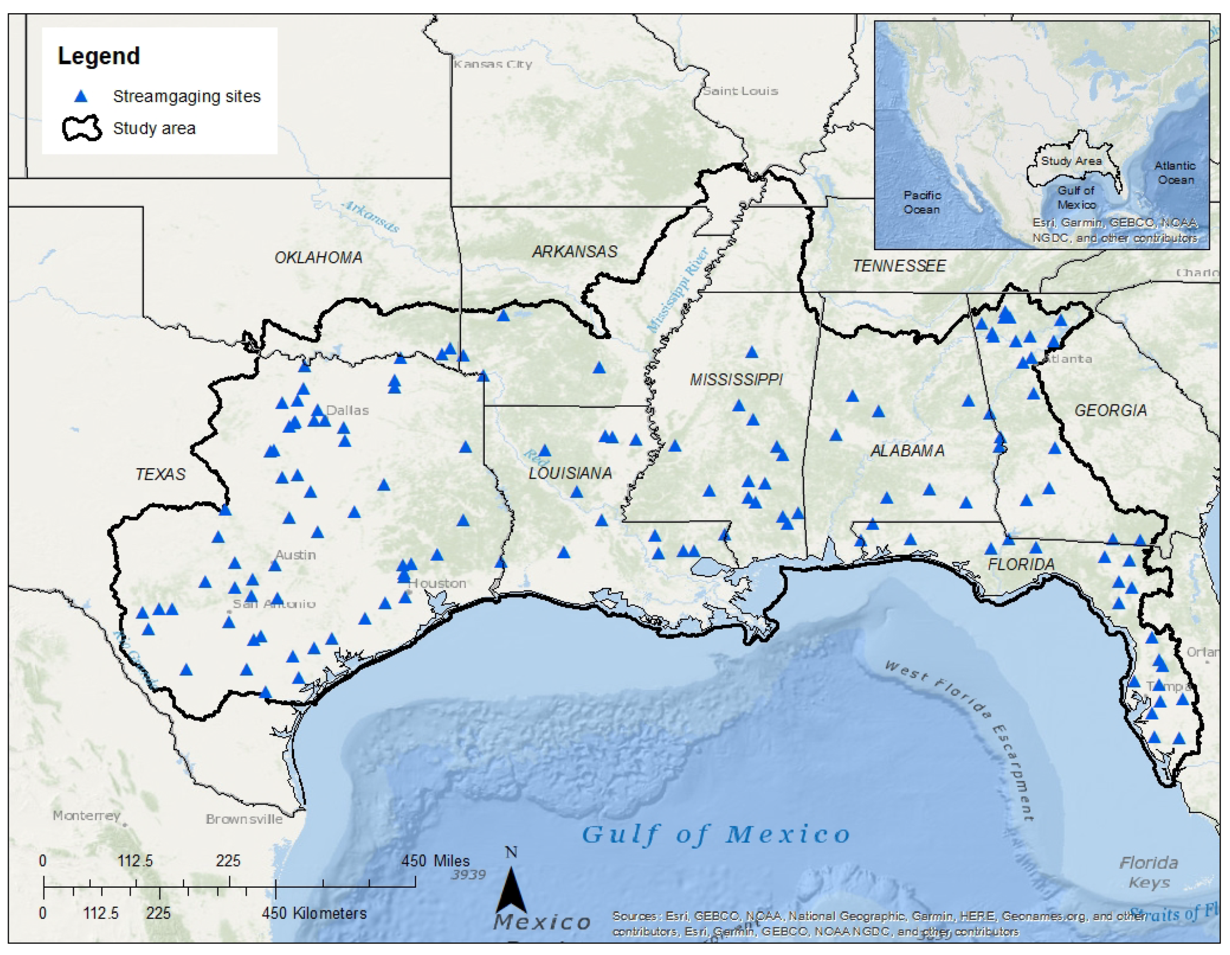
:In this article, the mean daily streamflow at 139 streamflow-gaging stations (sites) in the southern and southeastern United States are analyzed for spatial and temporal patterns. One hundred and thirty-nine individual time-series of mean daily streamflow were reduced to five aggregated time series of Z scores for clusters of sites with similar temporal variability. These aggregated time-series correlated significantly with a time-series of several climate indices for the period 1950–2015. The mean daily streamflow data were subset into six time periods—starting in 1950, 1960, 1970, 1980, 1990, and 2000, and each ending in 2015, to determine how streamflow trends at individual sites acted over time. During the period 1950–2015, mean monthly and seasonal streamflow decreased at many sites based on results from traditional Mann–Kendall trend analyses, as well as results from a new analysis (Quantile-Kendall) that summarizes trends across the full range of streamflows. A trend departure index used to compare results from non-reference with reference sites identified that streamflow trends at 88% of the study sites have been influenced by non-climatic factors (such as land- and water-management practices) and that the majority of these sites were located in Texas, Louisiana, and Georgia. Analysis of the results found that for sites throughout the study area that were influenced primarily by climate rather than human activities, the step increase in streamflow in 1970 documented in previous studies was offset by subsequent monotonic decreases in streamflow between 1970 and 2015.
1. Introduction
Significant changes in the natural streamflow regime for streams throughout the United States (U.S.) have been identified using analysis of spatial and temporal trends in streamflow [1,2,3]. These deviations, resulting from both anthropogenic and climatic influences, affect local communities and aquatic biology in many ways, including changes in streamflow, community composition, and alterations to habitat that are necessary to support indigenous wildlife. Given the variability in streamflow and the effect on the biological endpoint and community composition [4,5], there is a need for a more complete understanding of trends across the full streamflow regime, which can aid in understanding the effects of alteration on the water resource and its associated ecosystem.
Spatial variability in streamflow and the climatic, physiographic, and anthropogenic drivers of that variability are important aspects of streamflow trend analysis. Rice et al. [6] identified a spatial correlation of trends in watersheds of the U.S. and determined that in most ecoregions, mean annual precipitation has a strong, direct influence on changes in annual streamflow, but that the magnitude of the changes varied and was ecoregion dependent. McCabe and Wolock [7] examined the spatial correlation of trends and identified 14 clusters of streamflow-gaging stations across the U.S. with similar “temporal patterns.” The streamflow metrics varied seasonally and had a similar geographic distribution to that identified by Sagarika et al. [8]. Seasonal variability of trends in regions with similar geographic patterns was also identified by Dettinger and Diaz [9], who found similar spatial clusters of trends in streamflow.
In addition to anthropogenic effects (i.e., land-use and water-use driven changes or human-made alterations to a surface-water system), climatic oscillations may also alter the streamflow regime. Climate variability and changes to streamflow combined with increasing temperatures have greatly affected water availability [10], resulting in a reduced runoff on a local [11,12] and global scale [10]. Climatic oscillations in the Atlantic and Pacific Oceans have been shown to influence streamflow [13,14,15] in the eastern and western U.S., respectively. Cayan and Peterson [15] found that an offshore regional atmospheric circulation pattern was associated with streamflow change in British Colombia. They determined that the El Niño-Southern Oscillation (ENSO) tends to induce greater than normal streamflow in the southwestern U.S. Changes in the snow-rain melt or the frequency and/or increased magnitude of storms during climatic oscillation also influence the amount of water delivered to a stream [13,16]. Several studies, including works by Schulte et al., Mantua et al., Kahya and Dracup, and McCabe and Dettinger [17,18,19,20], suggest a “teleconnection” between climate oscillations and changes in streamflow. Milly et al. [21] suggested that the global pattern of observed annual streamflow trends is unlikely to have arisen from unforced variability and is consistent with modeled response to climate forcing.
In 2017, the U.S. Geological Survey (USGS), in cooperation with the U.S. Environmental Protection Agency, began a study as part of a broader effort by the Gulf Coast Ecosystem Restoration Council (RESTORE Council) to assess streamflow alterations and how they are related to bay and estuary restoration in the Gulf states (Alabama, Florida, Louisiana, Mississippi, and Texas). Whereas other studies have focused on only a few streamflow characteristics (e.g., in annual mean streamflow [22] or annual minimum, median, and maximum streamflow [7,23,24]), this study provides a more complete examination of changes in the distribution of streamflow throughout the year. Specifically, this examination includes: (1) The presence/absence of monthly and seasonal trends in streamflow from 1950–2015 at 139 streamflow-gaging stations (hereinafter referred to as sites) and 11 deciles of the streamflow (Q00–Q100) distribution to obtain a better understanding of how streamflow varies over time and over the full streamflow distribution; (2) the results of a cluster analysis of sites grouped based on their degree of similarity; (3) climatic oscillations and the correlation with streamflow; and (4) a relatively new methodology called the Quantile-Kendall analysis [25,26,27] to examine shifts in 365 points in the streamflow duration curve to derive a new picture of streamflow trends and the drivers of trends. Spatial patterns of streamflow trends are described for reference sites (minimally altered sites as determined by Falcone et al. [28]) in comparison to trends in a larger stream network that includes human land use and water-diversion effects to understand possible future changes in water-resource availability. This research will support subsequent analyses of quantifying streamflow alterations in the Gulf states.
2. Study Area
Located in the southern and southeastern U.S. and covering an area of approximately 442,000 mi2 (1,144,262 km2) with about 1650 mi (2655 km) of coastline, the study area includes all or parts of the five Gulf states in addition to parts of Arkansas, Georgia, Kentucky, Missouri, Oklahoma, and Tennessee (Figure 1). The study area is composed of 29 4-digit hydrologic units (HUC4) [29] ranging in size from 9506 mi2 (24,620 km2) (HUC 0312, Ochlockonee) to 73,345 mi2 (189,963 km2) (HUC 1211, Nueces-Southwestern Texas Coastal) (Supplementary Materials S1, Table S1). The highest elevation is in the mountainous region of northern Georgia at 4458 ft (1359 m) above sea level, and the lowest elevation in New Orleans, Louisiana, at 8 feet (1359 m) below sea level.
The study area is home to over 44,000,000 people [30], with approximately 4,000,000 people served by public supply utilities that rely on surface waters as their source of potable water [31]. The largest city by population (2,099,451; [30]) and area (599.6 mi2; 1553 km2) is Houston, Texas. The study area contains many major industries (e.g., oil manufacturing, shipbuilding, fisheries), tourism destinations, and agriculture, including cotton, rice, and wood products [32]. Surface-water withdrawals for public supply, which includes business, public facilities, and residential properties, total 4.34 million gallons per day (Mgal/day) (16,428.7 kiloliters/day) [31]. In landmass, the study area is one third the size of the Mississippi River basin and includes 23 ecoregions [33], 9 physiographic provinces [34], and 698 geological units [35].
Most of the study area is classified as a humid/subtropical climate [36]. The average temperature ranges from 54.5 degrees Fahrenheit (12.5 °C) in Missouri to 70.7 degrees Fahrenheit (21.5 °C) in Florida, and the annual precipitation ranges from 28.9 inches (734 mm) in Texas to 60.1 inches (1527 mm) in Louisiana [37]. Average precipitation is lowest in the western part of the study area, increases steadily eastward to western Georgia, then decreases eastward through central Georgia and parts of Florida. Areas closer to the coast experience heavy and frequent summer thunderstorms from tropical air masses; July and August are typically the wettest months, and precipitation is otherwise evenly distributed throughout the rest of the year. Summer dominance of precipitation increases gradually from the center of the study area towards the western and eastern edges. In central Georgia, less than 40% of annual precipitation falls during warm months, whereas in Texas and southern Florida, the fraction is greater than 70% [22]. Further from the coast, during winter and spring, the clashes between cold, dry air masses from Canada and warm, moist air masses from the Gulf of Mexico produce maximum precipitation during these cooler months in addition to hurricanes and tropical monsoons.
3. Materials and Methods
3.1. Data Preparation and Site Selection
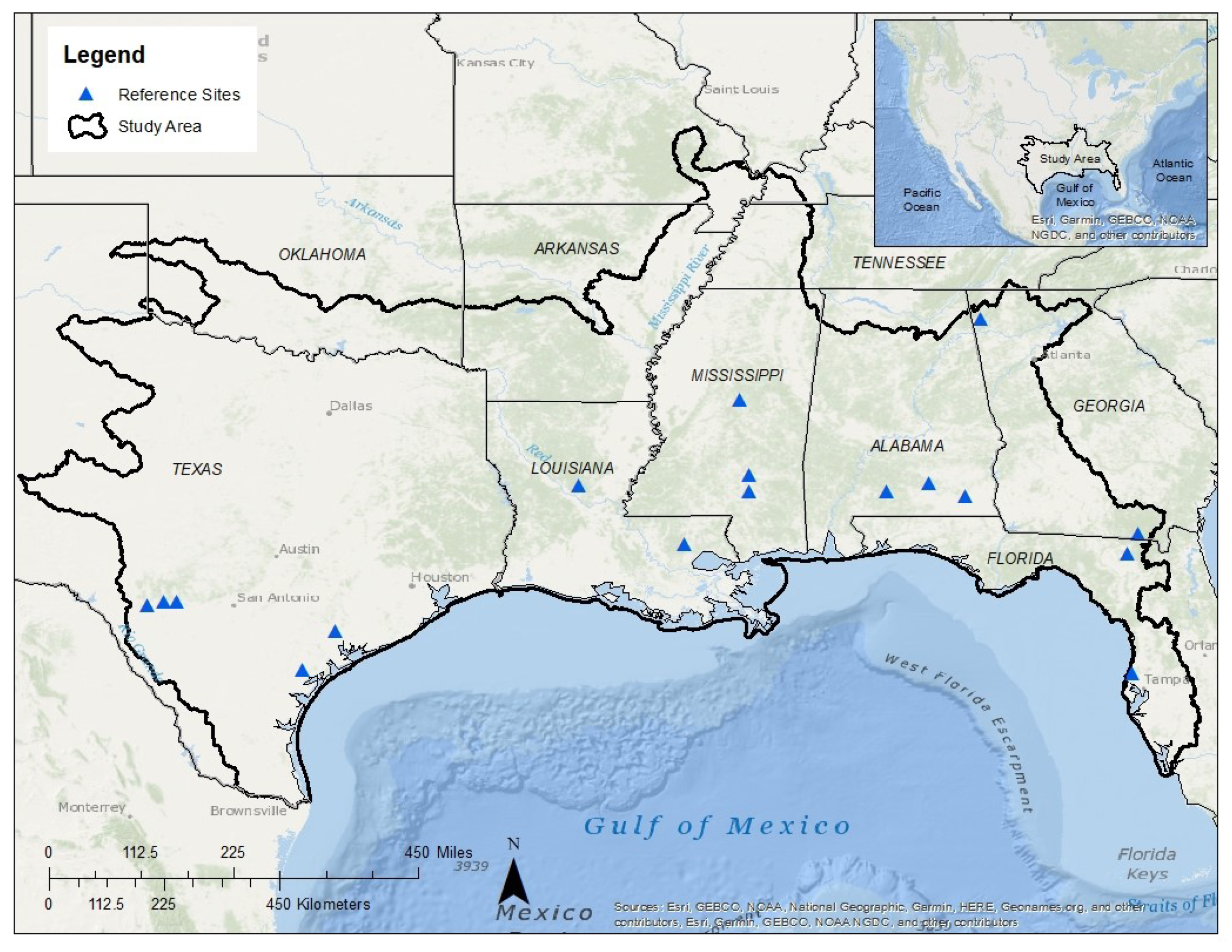
Mean daily streamflow data used in this analysis were downloaded from the USGS National Water Information System database [38] for 1371 streamflow-gaging stations in the study area. An analysis of streamflow data by decade identified 139 sites (Supplementary Materials S1, Table S1) with 66 years of daily streamflow values beginning in 1950. From the 1371 streamflow-gaging stations, sites were selected for this study if they had 99% of daily streamflow values during the period of analysis (1950–2015). A 66-year period of analysis yields 24,106 mean daily values for streamflow for each site. Included in the dataset are 17 sites (Figure 2) classified as “least disturbed” by anthropogenic changes as compared to other sites within an ecoregion [28]. These sites are referred to as reference sites, hereinafter (Supplementary Materials S1, Table S1).
3.2. Mann–Kendall and Correlation Analysis of Time-Series Data for Clusters of Sites
The methodology used in this study to group sites with similar temporal variability into clusters was derived from McCabe and Wolock [7]. The analysis is based on the Pearson correlation between time-series streamflow pairs for all sites transformed into Z-scores. The Z-score measures the distance from the mean to the data point and is denominated in standard deviations of the dataset. The Z-score can be a positive or negative value indicating that the value is either higher or lower than the mean of the dataset. Z-scores were used to decrease the influence of differences in streamflow magnitude (due to differences in drainage area) on the temporal variability in the dataset. The initial clustering process began with all of the selected sites in the study area. Pearson correlation with all sites in the region is significant (p < 0.05, α = 0.05) with a Pearson correlation coefficient above ρ = 0.50. Time-series of Z-scores for sites that share a stream reach are inherently not independent of one another, and as a result, these sites were significantly correlated, and therefore, were grouped in the same cluster. All the correlated sites in the first round of correlation analysis were clustered and removed from the larger set of sites.
Several sites were not included in a cluster after the first round of correlation analysis. To account for these sites, a second round of correlation analysis was conducted. Mean seasonal time-series of Z-scores were calculated for each cluster and tested with the Z-score time-series of sites not clustered in the initial round of the clustering procedure. In contrast to McCabe and Wolock’s approach [7], this analysis did not impose a minimum number of sites on the clustered groups; that is, all sites were included in a respective cluster. A time-series of seasonal mean Z-scores was calculated for each final cluster for use in the Mann–Kendall trend test and correlation analysis. Mean, median, and range statistics were calculated for each of the cluster time-series Z-scores.
The Mann–Kendall trend test [39] was used to identify significant trends in the mean seasonal time-series Z-scores for each cluster and the Pearson correlation coefficient (ρ) to quantify the relationship between two time-series Z-scores or how X1 varies with X2; in this case, the relationship between a cluster’s mean seasonal time-series Z-score and a selected climate index. Monthly time-series for climate indices were retrieved from the Royal Netherlands Meteorological Institute (KNMI) Climate Explorer [40]. The time-series of Z-scores for each cluster were tested for correlation against five climate indices: El Niño-Southern Oscillation 3.4 (ENSO) [41], North Atlantic Oscillation (NAO) [42], Pacific Decadal Oscillation (PDO) [18], Atlantic Multidecadal Oscillation (AMO) [43], and the Pacific-North American (PNA) index [44].
In general, climate indices are derivations of variability in sea-surface temperature (SST), but the NAO and PNA are exceptions [42,44]. The PNA index is derived from daily projections of mid-atmosphere (4980 m to 6000 m) anomalies on the pattern of monthly mid-atmosphere anomalies from 1950 to 2000, and the NAO index is based on the difference in the surface sea-level pressure between the Subtropical High (Azores) and the Subpolar Low. The AMO index is defined as the detrended 10-year running mean of SST anomaly north of the equator, the PDO index is defined as the principle component of the North Pacific monthly SST variability poleward of 20° N [44], and the ENSO is defined as five consecutive 3-month running mean anomalies of sea surface temperature anomalies above (below) the threshold of 0.5 C in the equatorial Pacific Ocean between the west coast of North America and the east coast of Asia.
3.3. Mann–Kendall and Quantile-Kendall Trend Analysis of Time-Series Data at Individual Sites
Analysis of streamflow time-series for monotonic trends (one direction, either increasing or decreasing) was performed using the non-parametric Mann–Kendall trend test [37]. The Mann–Kendall Trend test is a “rank-based” test [1] that determines not only the statistical significance of a monotonic trend in a measured attribute [45,46], but also the direction and magnitude (slope) of the change. Trend slopes are computed from each test using the Thiel-Sen slope estimator [47,48] and then transformed to percent change per year [25]. The Mann–Kendall trend test is not affected by extreme values or outliers and does not require the data to be normally distributed. It is assumed that some degree of autocorrelation is evident in Mann–Kendall trend analysis, however “pre-whitening” of the dataset can remove or inhibit the identification of trends in the data.
The Mann–Kendall test was also used to analyze trends over the full range of quantiles of streamflow distribution, termed the Quantile-Kendall (Q-K) analysis [26,27]. Q-K provides a more complete description of changes in the shape or magnitude of the annual or seasonal streamflow duration curve. Quantiles, as used in this context, are the boundary points that divide the observations in a sample into a set of intervals with equal numbers of observations in each interval. In a Q-K analysis for an annual time frame, the quantile boundary points divide the range of 365 daily values in each year into 365 intervals, each with 0.274% of the sample. Mann–Kendall trend tests are then applied to each of the 365 ranks (order) over a specified period of years. When a leap year is encountered, the 183rd and 184th ranked values are averaged. The analysis may be specified for a subperiod of the annual time frame as well: Q-K analysis for winter, for example, would divide the range of 92 daily values in each winter into 92 intervals, and apply Mann–Kendall trend tests to each of the 92 ranks over a specified period of years. A full description is given in Choquette et al. [27].
Results from the seasonal Mann–Kendall analysis for each of the 365 streamflow quantiles using the Q-K analysis [26,27] for each of the six multi-decadal trend analysis periods were combined for visual analysis and interpretation into a single graph, termed the stacked Quantile-Kendall (Q-K) graph. Each symbol (vertical line) on the graph represents the Mann–Kendall trend test result for each quantile (its position on the x-axis) and multi-decadal trend period (its position on the y-axis); symbol color is explained on the graph. A symbol plotting at the far left edge of the graph indicates a significant trend (p-value < 0.05; α = 0.05) for the annual time-series of lowest-ranked streamflow in the year (the annual minimum daily streamflow), whereas a symbol plotting in the middle of the graph from left to right, corresponding to the 50th percentile, indicates a significant trend of the 183rd ranked streamflow in the year (median streamflow). The absence of a vertical line, equivalent to a white vertical line, at a percentile of flow duration means that no significant trend was detected for that quantile. Results for all six trend periods are stacked vertically in the graph: Symbols plotting in the region near the bottom of the graph, corresponding to starting in 1950, indicate significant trends for the 66-year period 1950–2015; symbols plotting near the top of the graph, corresponding to starting in 2000, represent significant trend test results for the 16-year period 2000–2015 (all periods for trend testing ended in 2015). In this analysis, it was assumed that observations of significant trends across the streamflow regime were independent of one another. The individual rankings of significant trends across the full range of streamflows at a site were not tested for independence, and as such, the statistical significance of the results must be caveated with this condition. It is important to note that the p-values do not show the same significance one would usually expect and that there is the autocorrelation of points in the Q-K analysis and the ranked values. As a result, quantifying the true significance of trends at a streamflow exceedance probability is difficult because the ranked trend is a portion of the greater trend in the streamflow regime. All data used to support the analysis and create the graphs in this paper are available from Rodgers et al. [49].
3.4. Comparison of Each Site’s Trend Results to Reference Conditions
The Q-K trend analysis results for each site were compared to the Q-K trend analysis results for a companion reference site (Figure 2) to infer the extent to which temporal variation of streamflow at the non-reference sites (Figure 1) were due to temporal variation of climatic factors as opposed to land use, water use, or any streamflow alterations within the watershed. The climate clusters used to pair non-reference sites with the appropriate reference site for the Q-K result comparisons were derived from the cluster analysis described in a previous section. The Q-K result comparison between non-reference and associated reference sites is summarized as the metric Trend Departure Index (TDI), computed as:
where n is the number of quantiles for which the trend result for a non-reference site departs from the result for the associated reference site divided by 365, which is equal to the total number of quantiles in a Q-K analysis for the annual time frame.
TDI varies from 0 to 1; a TDI of 0 indicates the trend results for the site are identical to the reference site, and any value larger than 0 indicates some departure compared to the reference condition. The larger the number (closer to 1), the more departure or deviation relative to the reference site in trend across all the quantiles for the site. The trend components that diverge from the climate-driven pattern as defined by the assigned reference site can be interpreted as changes through time in human activities in the watershed. For the purpose of a qualitative description of the results in this study, a value of 0.44 (based on interquartile ranges of sets of results) was assigned as the upper threshold of similarity to reference conditions; that is, sites are described as having trend results similar to reference conditions, and by inference, the observed trends at that site are assumed to have been largely driven by climate influence, if TDI ≤ 0.44. Conversely, large numbers for TDI, ≥0.67, are interpreted to mean that the main drivers for observed trends in streamflow at the site are changes in anthropogenic factors.
4. Results and Discussion
4.1. Cluster Analysis and Trends in Cluster-Mean Time-Series
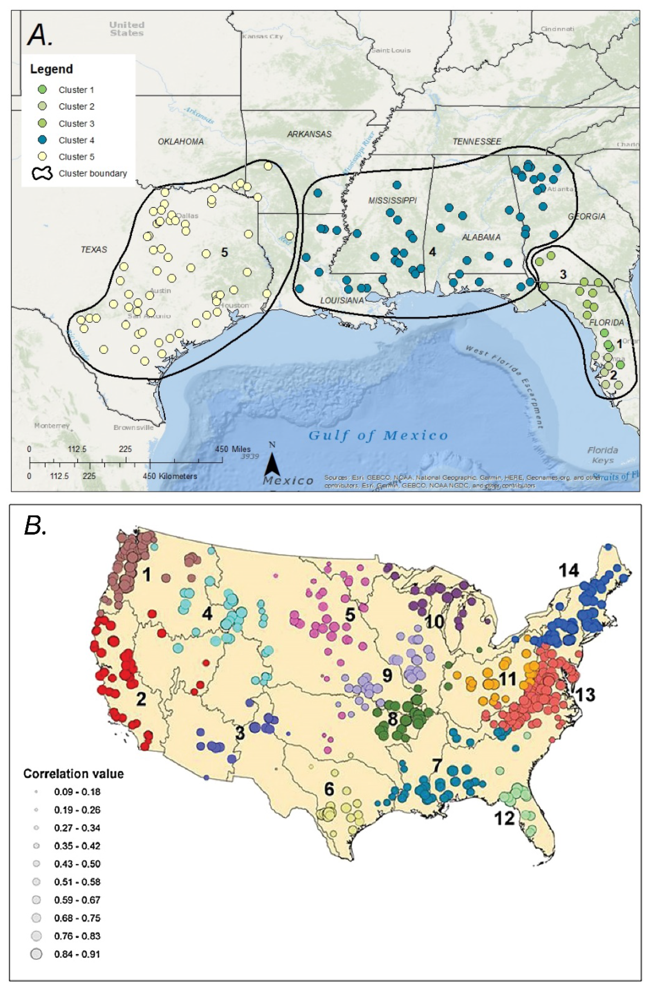
The data reduction clustering analysis identified five clusters, shown in Figure 3A; for comparison, clusters of sites with similar temporal variations in streamflow identified by McCabe and Wolock [7] are shown in Figure 3B. Sites included in cluster 1 (four sites) were in west-central Florida, cluster 2 (six sites) were in inland central Florida, and cluster 3 (ten sites) included sites in northern Florida and southern Georgia. The ten-site limit imposed by McCabe and Wolock [7] created their cluster 12, which roughly corresponds in location and in size with the combined clusters 1, 2, and 3.
Clusters 4 and 5 were the largest clusters identified, with 55 and 64 sites in each cluster, respectively. Sites in cluster 4 (which corresponds roughly with McCabe and Wolock’s [7] cluster 7) were in western Georgia and extended as far west as Louisiana. Sites in cluster 5 (which corresponds roughly with McCabe and Wolock’s [7] cluster 6) were in western Louisiana and extended to the far western boundary of the study area.
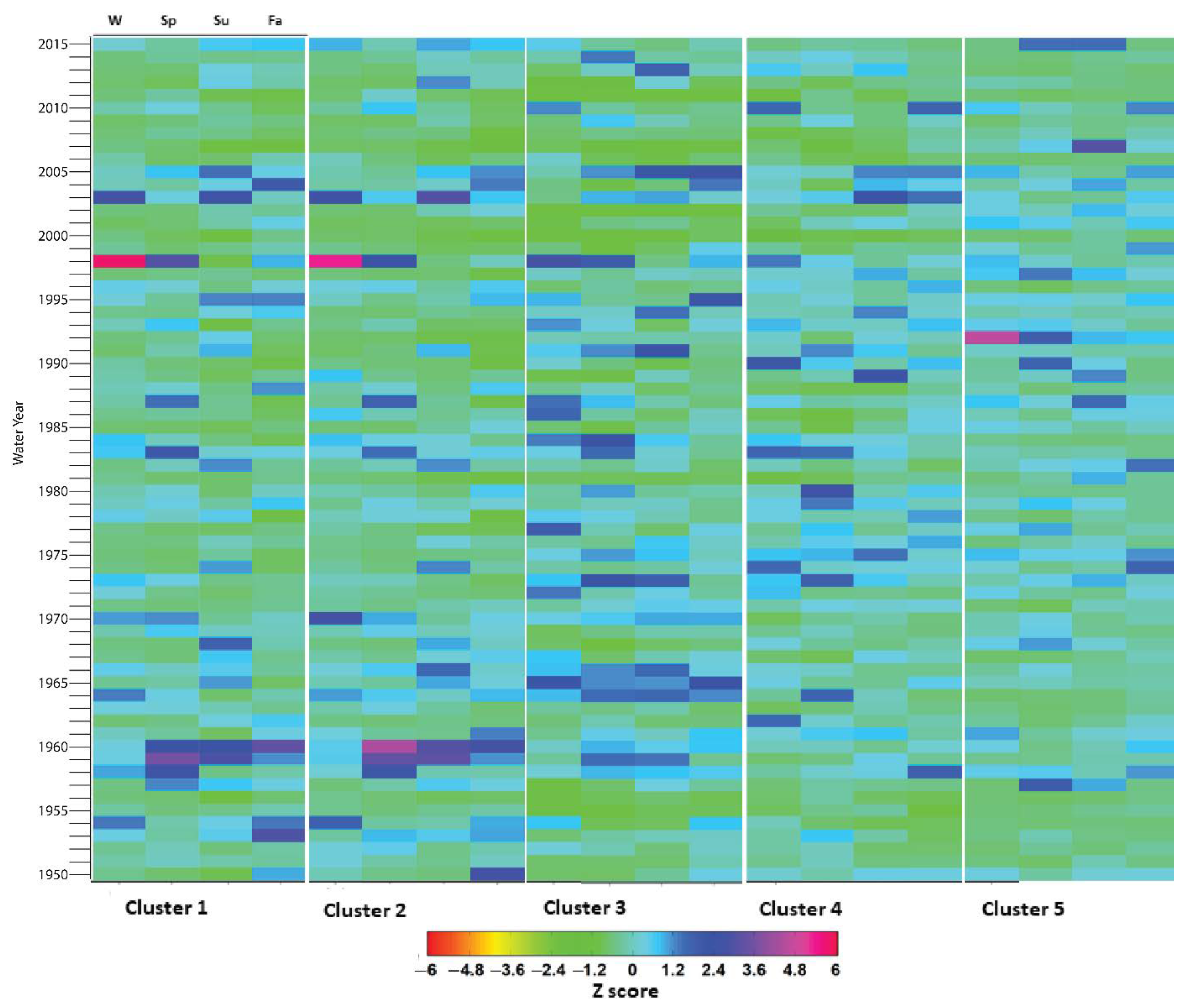
The mean time-series Z-scores for each cluster were within a range of −1.44 to 5.77. Cluster 1 had the largest range of Z-scores (4.64), and cluster 4 had the smallest range (1.086). Median Z-score values were similar for each cluster, which indicated sites in each cluster were similarly distributed around the cluster time-series of seasonal mean Z-score (Figure 4). Clusters 1, 2, and 3 each had relatively high Z-scores from 1957 to 1960, 1998, and again from 2003 to 2005, indicating streamflow was greater than one standard deviation from the long-term average. These instances typically occur over multiple seasons: Spring, summer, and fall during the period from 1957–1960, winter and spring in 1998, and throughout entire years from 2003 to 2005. In the winter of 1998, clusters 1 and 2 had unusually large Z-scores, possibly due to record rainfall in central Florida and other areas in the Southeast [50].
The patterns observed in clusters 1, 2, and 3 correspond to the seasonal distribution of precipitation (mostly occurring in the winter and spring months). Clusters 4 and 5 generally had more variable Z-scores; however, the values were typically above the long-term average from 1973 through 2005. A similar pattern occurred in cluster 3 over the same period. The boundaries of the clusters derived from the cluster analysis are considered to delineate areas of relatively homogeneous climate patterns, including in the temporal variation of climate, and therefore, to delineate areas within which trends in climatic drivers have produced similar trends in streamflow patterns. This result corresponds with McCabe and Wolock’s [24] findings of a step increase in streamflow in the 1970s.
Results of the Mann–Kendall trend test of Z-scores of streamflow from each cluster of mean seasonal time-series data (1950–2015) indicated that clusters 1, 2, and 3 each had significant decreasing trends over the period of analysis, and cluster 5 had a significant increasing trend (p < 0.05, α = 0.05). Cluster 4 did not have a significant trend (Table 1). In addition, the magnitudes of the Sen’s slope values were small for all clusters, an indication of a very gradual trend (increasing or decreasing). The lack of a significant increasing or decreasing trend for cluster 4 may reflect an even balance between sites in the cluster with increasing and decreasing trends; its location between clusters 1, 2, and 3 to the east, which corresponds with cluster 12 from McCabe and Wolock [7] (decreasing trends), and cluster 5 to the west, which corresponds with cluster 6 from McCabe and Wolock [7] (increasing trend), reinforces even balance as a possible explanation.
4.2. Correlation between Seasonal Time-Series of Cluster-Mean Streamflow and Climate Indices
The five climate indices only explained a small fraction of the variability in the mean seasonal streamflow at sites within the clusters, which is a result that corroborated the findings in McCabe and Wolock [24]. Streamflow increased at sites in the clusters as the value of the PDO index increased, and clusters 1 and 5 had the most significant correlation with the PDO (Table 2). Correlations were positive and statistically significant (p-values < 0.05, α = 0.05) between cluster time-series Z-scores and the PDO, except for clusters 4 (Table 2). The correlation between all clusters and the PDO had similar values, which indicated that the effect of changes in the PDO on streamflow was similar for each cluster, albeit the correlations were weak.
Similar to the correlation with the PDO, the correlations between the seasonal cluster time-series Z-scores and the seasonal time-series ENSO index were statistically significant (p-value < 0.05, α = 0.05) in clusters 1–3 and 5. Similar results for ENSO and PDO were expected because the ENSO and PDO indices are both based on SSTs in the Pacific Ocean; however, the PDO is based on the long-term decadal mean of SSTs, whereas ENSO is based on the monthly mean. There has been a longstanding debate in the field of climatology about the relationship between ENSO and PDO and the mechanisms driving their respective modes, as well as their independence from one another.
In a study exploring the effect of ENSO on drought in the continental U.S., Rajagopalan et al. [51] and Tuttle et al. [52] described the PDO as having no significant moderating effect on ENSO over most of the continental U.S. Studies by Juanxiong et al. [53] and Hamlet and Lettenmaier [54] reached similar conclusions. The findings are in contrast to the findings of Gershunov et al. [55] that determined the PDO was responsible for the modulation of ENSO-related winter precipitation in the U.S. Studies conducted by Allan et al. [56] and Verdon et al. [57] also concluded that the PDO and ENSO were related; however, the multi-decadal period of the PDO described several relatively short-term ENSO events. The results of this study suggest agreement with these findings [55,56,57].
Sites located in the western and central part of the study area (clusters 4 and 5) and in northern Georgia (Cluster 3) were significantly correlated (negatively) with the AMO (p-value < 0.05, α = 0.05). This result agreed with the results of Enfield et al. [58] that described continental-scale patterns of negative correlations between rainfall and the AMO index. In contrast to sites in the eastern part of the study area (clusters 1 and 2) (Table 2). The correlation between seasonal streamflow and the AMO was most significant at sites in Cluster 3. Over the study period, the mean of the AMO was slightly negative but near zero. Based on this result, streamflow in the clusters that were correlated with the AMO tended to vary inversely, resulting in increasing streamflow as the AMO index decreased. There was no significant correlation between the cluster time-series Z-scores and the NAO. The PNA index had a significant positive correlation with each cluster, except for cluster 4—which is likely a result of the wide-ranging, but subtle influence the PNA has on the ENSO, PDO, and AMO climate indices (Table 2).
The climate indices explained approximately 8% or less of the variability in streamflow in the five clusters. The PDO explained from 1.1% to 4.26% of the variability in the cluster time-series Z-scores; the AMO between 0.3% and 7.63%, the NAO 0.26% or less, the ENSO between 1.23% and 5.3%, and the PNA between 0.07% and 3.97% (Table 3). Because of the shared relationships between the climate indices and global SST, the cluster time-series Z-scores were tested against a field of mean seasonal global SSTs for the period of this study to identify potential teleconnections between ocean regions around the globe whereby SST and streamflow in the clusters were directly correlated.
Clusters 1 and 2 had similar patterns of spatial correlation with SST characterized by positive correlation along the west coast of North America and in the equatorial Pacific Ocean (Figure 5; Supplemental Material S1, Figure S1A–E). Other areas of positive correlation included the British Isles, the mid-Atlantic, the Gulf of Mexico, the Caribbean Sea, and off the coast of Antarctica. Negative correlations between SST and streamflow for clusters 1 and 2 were generally found to occur in a band that wrapped around the globe between 30° S and 60° S. There was also a negative correlation with streamflow above 60° N in the Arctic Circle for clusters 1 and 2. The pattern of spatial correlation between streamflow in cluster 3 and global SST displayed the most correlation with oceanic regions around the globe. The pattern could be described as a more extreme version of the patterns observed in clusters 1 and 2.
Streamflow was positively correlated with SST in the northern and southern equatorial regions of the Pacific Ocean from the west coasts of Central America and South America in all clusters. A negative correlation between SST and streamflow was observed along the east coast of Asia, and in the waters off of the eastern and southern coasts of Australia, and in the South Pacific Gyre (cluster 1–4). There were also large regions of negative correlation that extended across the eastern seaboard of the U.S. and across the Atlantic Ocean to the British Isles. Cluster 4 was correlated with relatively fewer ocean regions around the globe. SST and cluster 4 streamflow were positively correlated in the Northern Pacific Ocean along the west coast of the U.S. and to some extent in the equatorial Pacific Ocean. Negative correlations were located in the central Pacific Ocean in the subtropics of the northern hemisphere and in the northern Atlantic near the British Isles. Cluster 5 was positively correlated with SST in more oceanic regions than what was observed with the other clusters. Streamflow from cluster 5 was positively correlated with SST along the equator, in the south Pacific Ocean, along the east coast of South America, and in portions of the Indian Ocean. There was a relatively small group of areas where cluster 5 streamflow and SST were negatively correlated. These areas included small regions of the North Atlantic and in the extratropic north-central Pacific Ocean.
4.3. Trends in Monthly Mean Streamflow
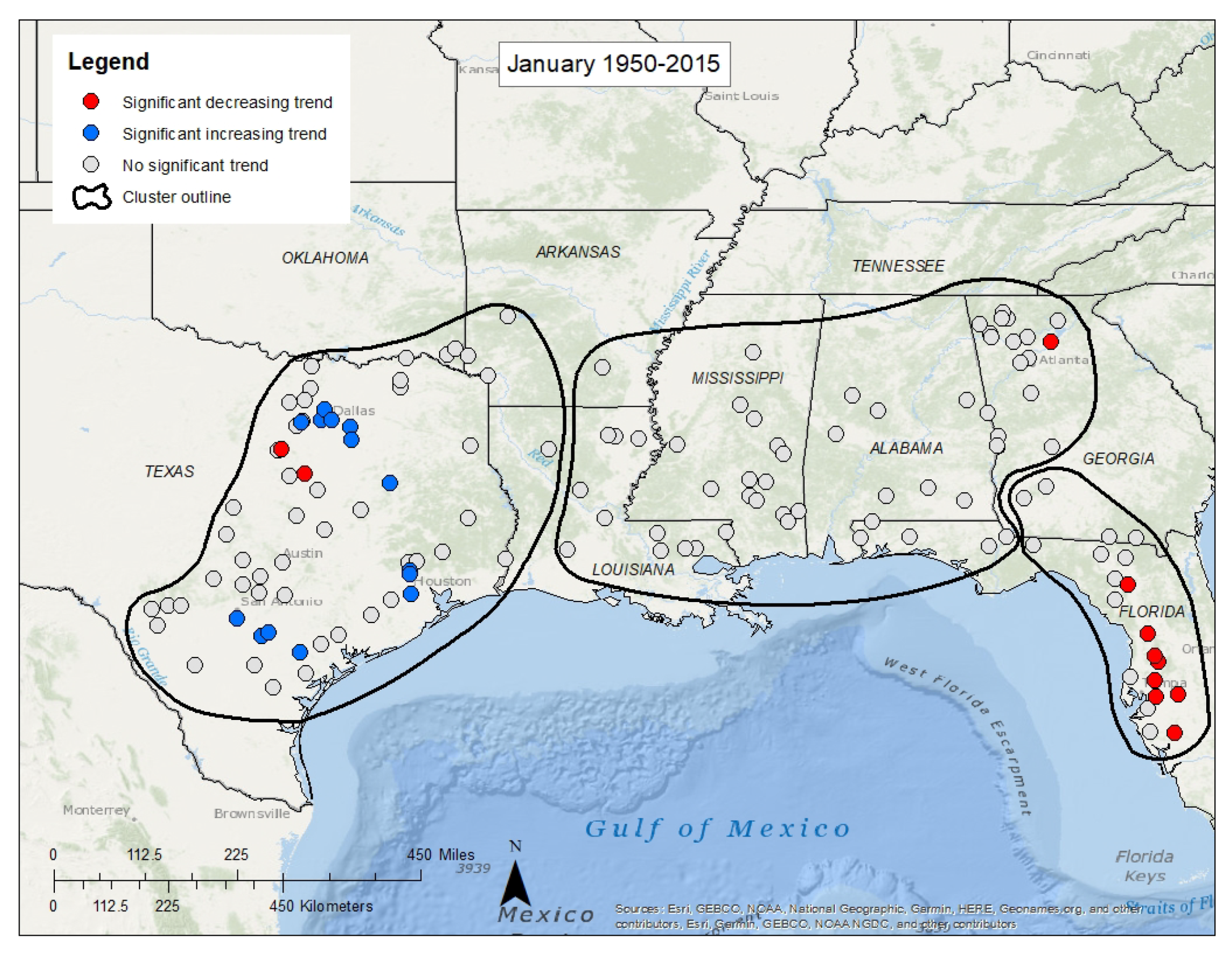
Maps depicting results from all monthly analyses can be found in Supplementary Materials S1, Figure S2A–L. For the period of analysis 1950–2015, March had the highest number of increasing trends (29), and May (4) had the lowest number of increasing trends (Table 4). Overall, March had the highest number of statistically significant trends (44), and June had the lowest number (20). From 1950–2015, increasing trends outnumber decreasing trends in all months except February, April, May, and June. Visual analysis of January results shows a clear geographic difference between increasing and decreasing trends (Figure 6). Decreasing trends are found in the eastern part of the study area, whereas all but two statistically significant trends in the western part of the study area are increasing. Analysis of the May 1950–2015 results indicate statistically significant decreasing trends cover the entire study area except for southern Texas (near Houston and San Antonio).
Of the four months where significant decreasing trends outnumber significant increasing trends, June trends are more balanced geographically with increasing and decreasing trends in both the eastern and western parts of the study area. In the western part of the study area (Texas), increasing trends are intermixed spatially with decreasing trends; however, in the east, as with the April and May results, decreasing trends are clustered around Tampa-St. Petersburg. From 1960 onward, statistically significant decreasing trends account for most of the monthly trends over all periods of record (Table 4). During the multi-decadal periods of 1970–2015, 1980–2015, and 1990–2015, decreasing trends account for all statistically significant trends in the months of January, February, and May (Table 4).
4.4. Trends in Seasonal Mean Streamflow
The largest number of significant trends in seasonal mean streamflow (1950–2015) occurred in the Fall season (Table 5). Decreasing trends in seasonal mean streamflow were predominant, outnumbering increasing trends by approximately 5 to 1. For the period 1950–2015, Fall had the greatest number of increasing (30) and decreasing trends (18). Spring had the smallest number of increasing trends (9), and summer and winter had the smallest number of decreasing trends (11). All of the decreasing trends identified for winter occurred in the eastern part of the study area (Florida), and all the increasing trends occurred in the western part of the study area (Texas) (Figure 7).
Overall, a pattern of decreasing streamflow trends was identified in the eastern part of the study area during all seasons from 1950–2015 (Supplementary Materials S1, S3A–D). Decadal variations in statistically significant trends by season are most apparent in trends identified in Fall. Increasing trends decline substantially in the Fall over the inter-decadal periods analyzed with 30 increasing trends identified in the 1950–2015 period of record to zero increasing trends in the 2000–2015 period of record. Over all periods of record analyzed, decreasing trends outnumber increasing trends, and in several instances, account for all significant trends identified in this analysis.
4.5. Trends in 11 Deciles of Annual Streamflow at 139 Streamflow-Gaging Stations
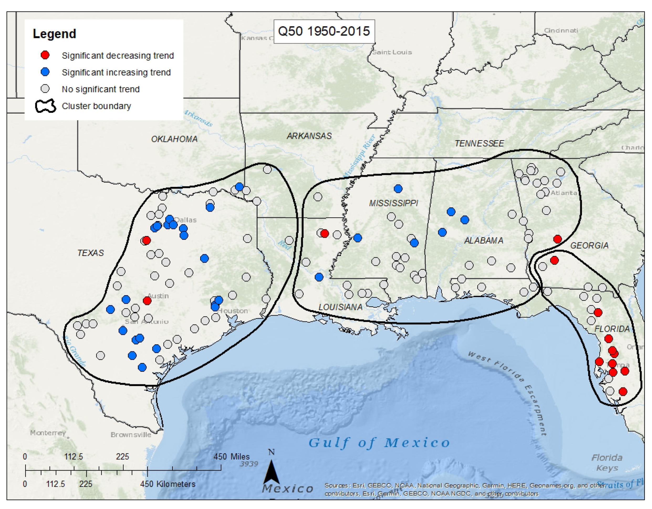
Results of a decile trend analysis suggest that, over the full streamflow regime, streamflow is decreasing, and as a result, the overall volume of streamflow to the Gulf of Mexico is decreasing. The minimum mean daily streamflow (Q00; low flow) had the largest number of significant trends (70) for the period of analysis 1950–2015 (Table 6). The number of statistically significant trends in Q00 ranged from 82 (59% of the sites) for 1970–2015 to 21 (15% of sites) for 2000–2015. On average, decreasing trends exceed increasing trend by approximately 4 to 1 over all periods analyzed. Decreasing trends were detected in low-to-middle ranges of streamflow (Q00 to Q50) consistently for sites throughout the eastern third of the study area, whereas decreasing trends in the higher deciles of streamflow had a narrower geographic range confined mostly to Florida (Figure 8, Supplementary Materials S1, Figure S4A–K).
4.6. Trends in the Full Range of Streamflow Quantiles (Quantile-Kendall Analysis)
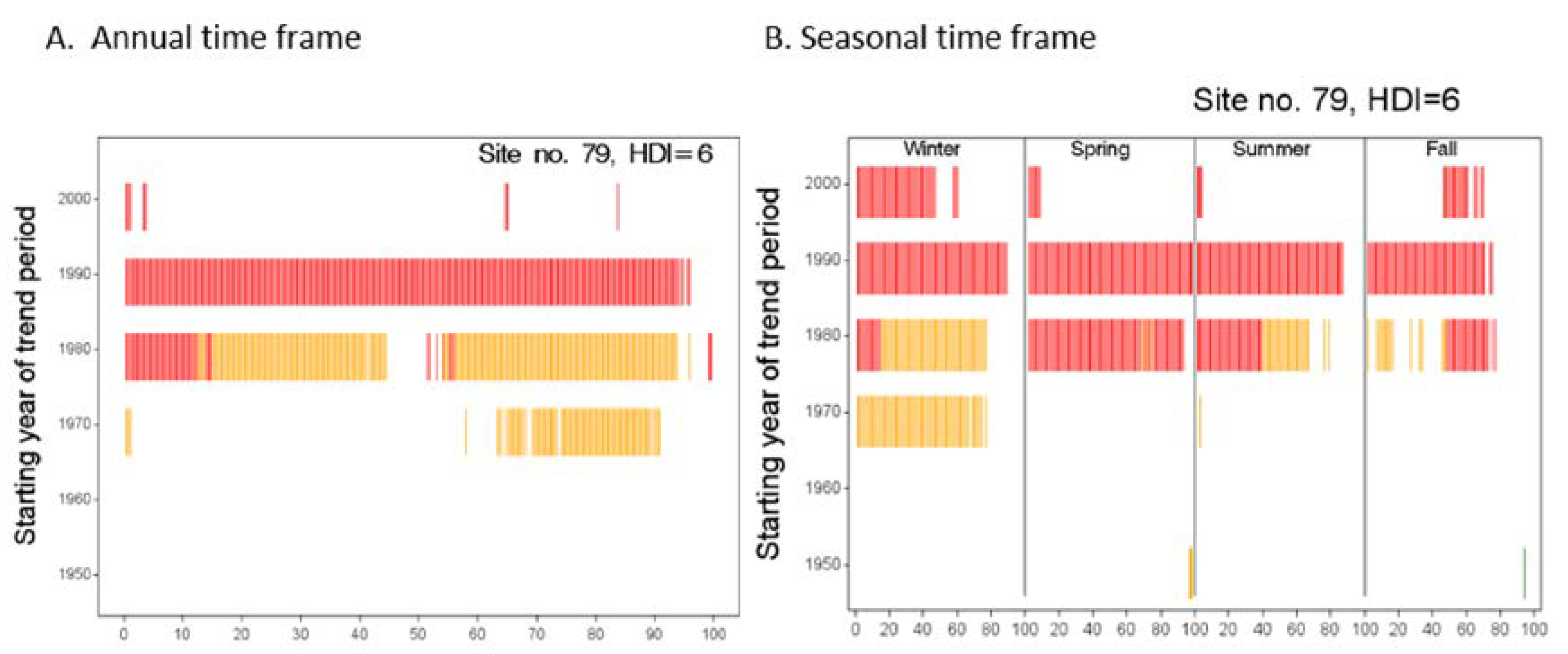
An example application of the stacked Q-K graphs for a site in Louisiana (site no. 79; Supplementary Materials S2) shows significant decreasing trends were detected in the annual minimum daily streamflow for four of the six trend periods, and decreasing trends were detected for almost all 365 percentiles of streamflow for the 25-year period 1990–2015 (Figure 9A). The overall pattern in observed trends for this site—a reference site—is inferred to represent the effects of temporal variation in the climatic factors that affect streamflow, without influence from temporal changes in human land use or water use in the watershed. The seasonal stacked Q-K graph (Figure 9B), provides additional information about the observed decreasing trend in streamflow of higher percentiles for the 1970–2015 period (shown in Figure 9A); specifically, that the results apply to winter streamflow only. Data to create the annual and seasonal Q-K graphs for all 139 sites are available from Rodgers et al. [49].
4.7. Spatial Variation in Streamflow Quantile Trends for Reference Sites (Reflecting Temporal Variation in Climate)
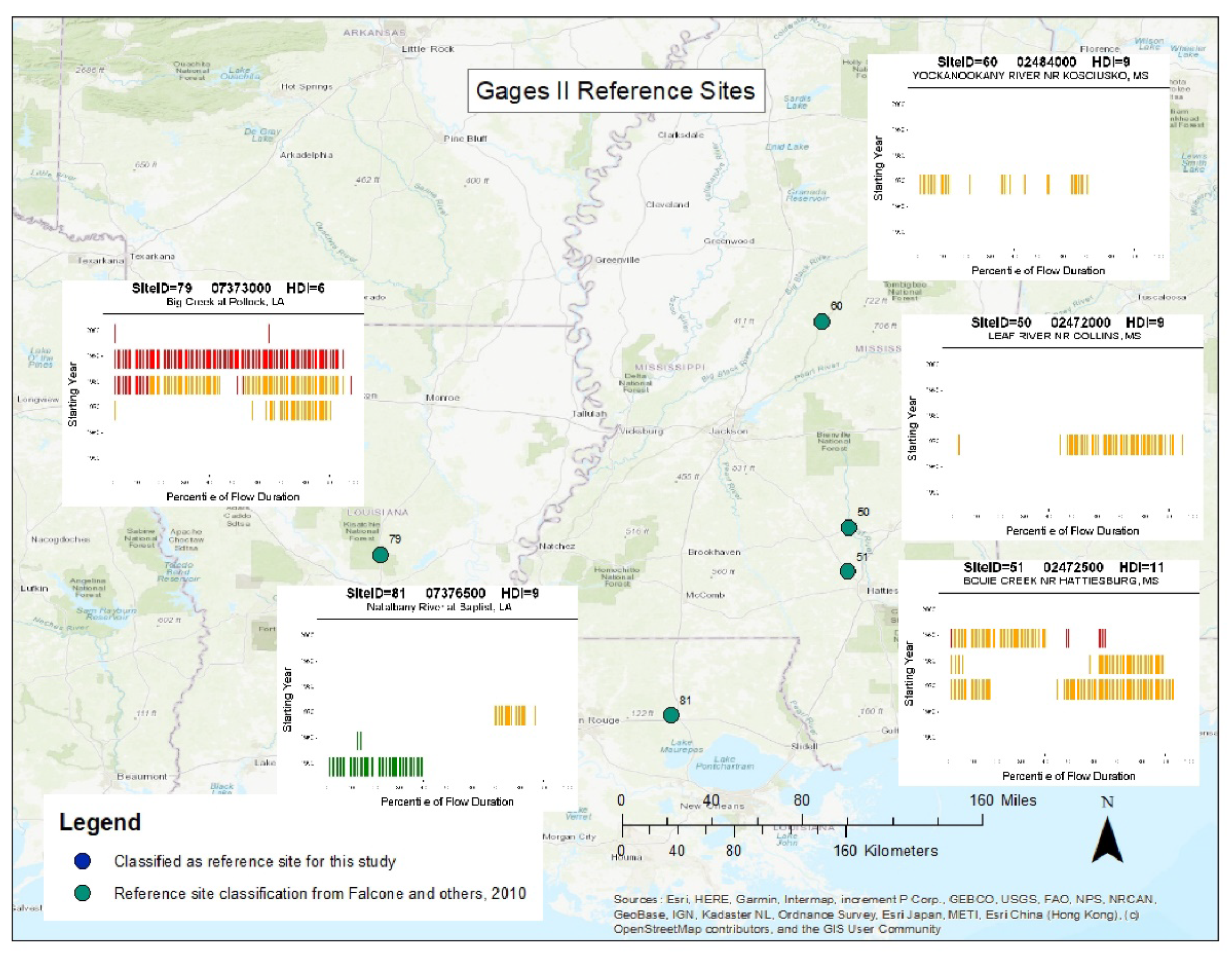
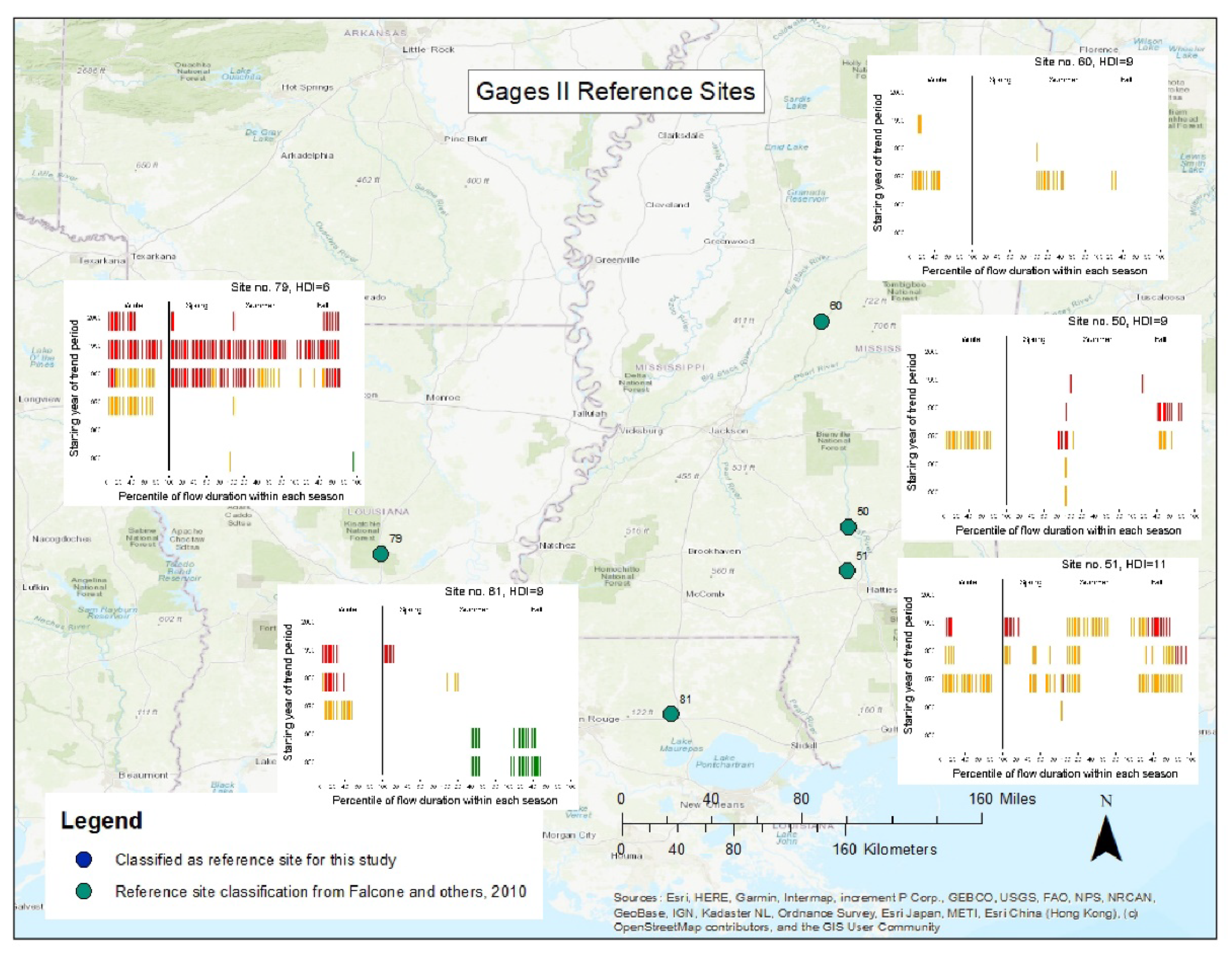
Trends at the 17 reference sites were significantly decreasing (p-value < 0.05, α = 0.05) except for one site located in Louisiana (Figure 10 and Figure 11; Supplementary Materials S1, Figure S5A–D; Supplementary Materials S2). The predominance of significant decreasing trends at all reference sites and for all trend periods during both the annual and seasonal time frames is striking. Decreasing trend slopes vary across the study area (slope percentage > 3% annually in Texas). The trend slope of reference sites in Mississippi and Louisiana (Figure 10) indicates shallow decreasing trends (<2% change) for the longest trend period. The number of decreasing trends in the shorter trend periods indicate a significant decrease in streamflow beginning in 1980. The single exception is for site no. 81 (USGS station no. 07376500 Natalbany River at Baptist, Louisiana) for which increasing trends were detected for low streamflow percentiles for the longest trend periods, and in summer and fall only (Figure 11).
For most reference sites in clusters 4 and 5, conditions were drier in 2015 than in 1970, but about the same as in 1950. The conspicuous lack of decreasing trends for the 66- and 56-year trend periods (periods starting in 1950 and 1960) despite the presence of decreasing trends for periods starting in 1970 and later is consistent with the theory that the one-time step increase in precipitation and streamflow that occurred rather abruptly near the year 1970 documented by McCabe and Wolock [24] has acted to balance the strong and consistent decreasing trends in streamflow detected for the 46-year and shorter periods (starting in 1970 or later), so that no net change is detected when analyzing for the 66- and 56-year trend periods.
Although it seems contradictory that environmental factors that influence streamflow changes at reference sites—presumably climate or other atmospheric factors—would create these two opposing directions of change, it is possible that a change in one set of atmospheric factors in or around 1970 produced the step change, while a change in a different set of atmospheric factors has produced the consistent decreasing streamflow trends observed since 1970 (for example, see the discussion in Krakauer and Fung [22]).
Spatial coherence of trends for the reference sites within a cluster improves when the distance from the coast is considered: For example, the reference sites (Supplementary Materials S1, Table S1) furthest from the coast in cluster 4 have fewer significant trends that are mostly confined to the 1970–2015 period, compared to reference sites closer to the coast. The proximity and possible spatial dependence (although on independent streamflow paths) of three of the five reference sites in the western part of cluster 5 are not ideal for evaluating spatial coherence for this cluster. As with cluster 4, distance from the coast may explain different patterns: Significant trends occur throughout the streamflow distribution and for three or more of the trend periods for the three sites in the western part of cluster 5, whereas trends are less common in trend periods with earlier starting years (before 1980) for the two reference sites near the coast.
The reference site sets are not ideal as streamflow patterns for paired reference sites on the same streamflow path, such as the Suwanee and Leaf Rivers (Supplementary Materials S1, Table S1), are likely to be autocorrelated unless intervening drainage renders them effectively independent. Because spatial correlation would invalidate conclusions about spatial coherence of reference site patterns, the sufficiency of intervening drainage area was analyzed to eliminate sites that could not be considered as independent observations; all reference sites were found to be sufficiently independent.
Several aspects of the trend results vary from east to west in the study area.
- Steepness of trends: Clusters 1, 2, and 3 (Supplementary Materials S2) have very few significant trends, but the slopes of the trends are steep (>2% change per year). In cluster 4, closer to the coast, the significant trends for longer trend periods tend to be shallow, whereas the slopes of significant trends for shorter, more recent trend periods (1980–2015 and 1990–2015) tend to be steeper. This is especially evident in the results of the seasonally stratified Q-K (likely due to the same factors that caused fewer significant trends for longer periods). In cluster 5, all slopes of significant trends are steep.
- Number of significant decreasing trends in higher streamflows (Supplementary Materials S2): Almost no trends in high streamflows were identified for sites in clusters 1, 2, and 3. Trends in high streamflow were present at some (5) sites in cluster 4, and in cluster 5 all reference sites show decreasing trends in high streamflows.
- Occurrence of trends in summer and fall streamflows (Supplementary Materials S2): Every reference site in cluster 5 had a significant decreasing trend in fall streamflow. Perhaps the dominance of precipitation (as high as 70% of the annual total) during warmer months and the resultant evapotranspiration combined with water use in this region makes streamflow more sensitive to changes in climate, hence steeper slopes, and more significant trends.
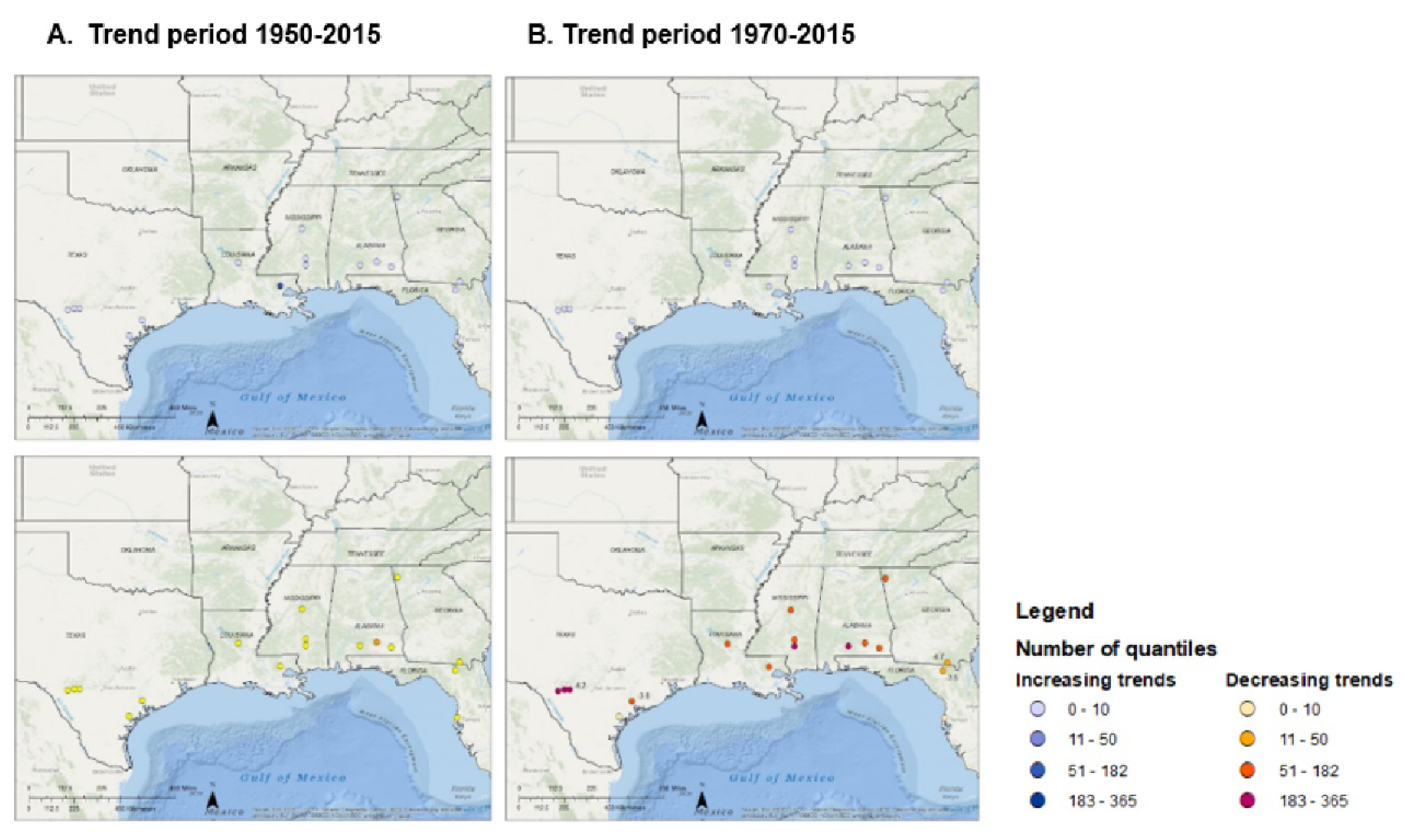
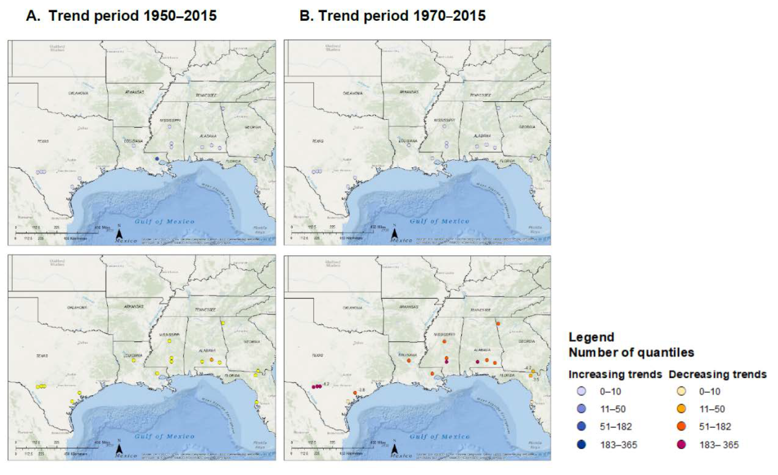
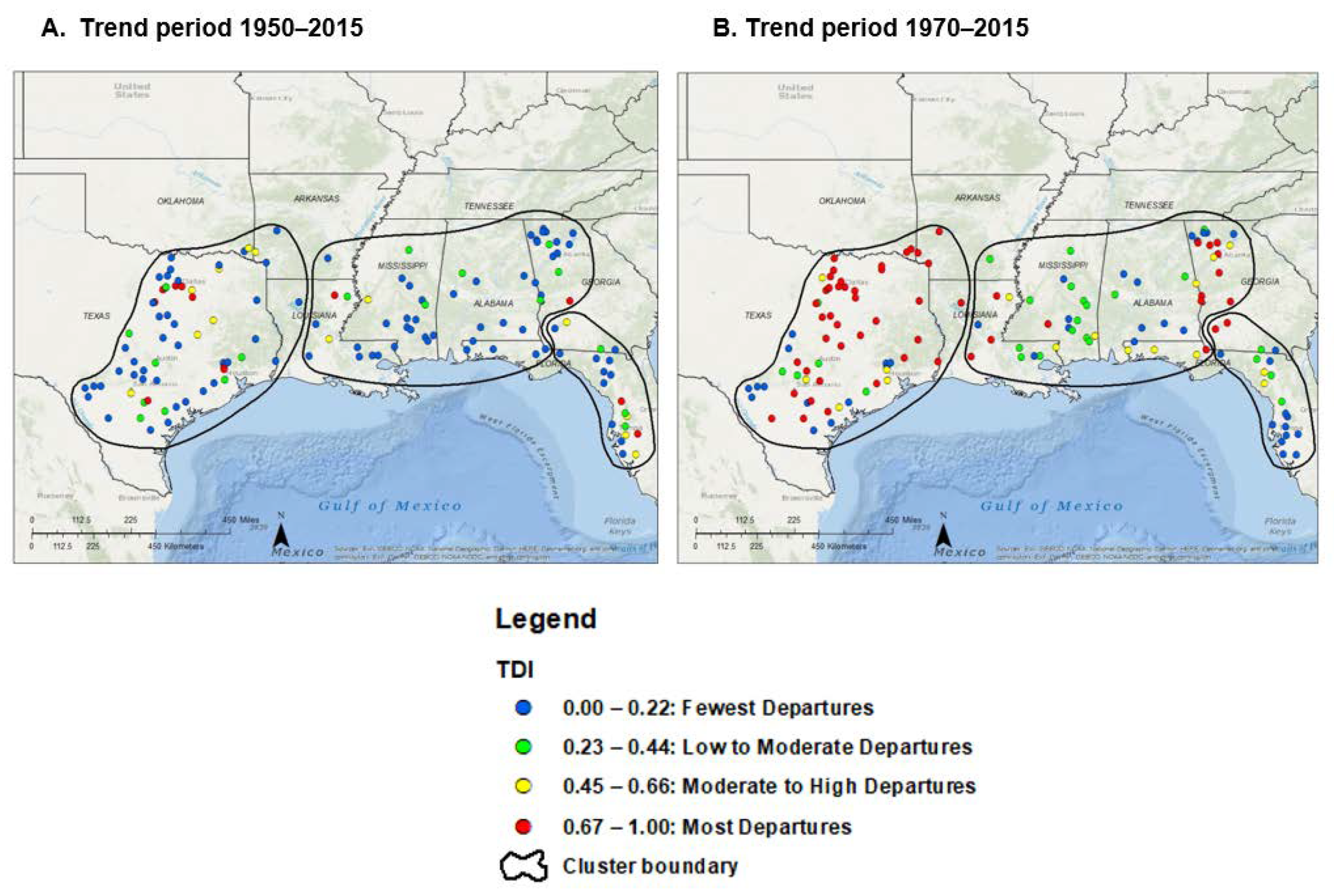
This analysis offers a more complete description than previous studies that have examined trend results only in mean values [22] or in minimum/median/maximum values [24]. The results illustrated in the stacked Q-K graphs were condensed to four metrics for each site and multidecadal period—the counts of quantiles with significant increasing and decreasing trends, and the mean value of trend slope for increasing and decreasing trends. For example, for site no. 79, Big Creek at Pollard, Louisiana (Figure 9A), the count of quantiles for the period 1970–2015 is 0 increasing trends (mean slope = 0) and 97 decreasing trends (mean slope = −1.0). Although these simple metrics lack detailed information on the location of the trend in the streamflow distribution, they are more suitable for quantitative comparisons between sites and clusters. The spatial distribution of the four metrics is shown in Figure 12A,B, for the periods 1950–2015 and 1970–2015, respectively. These two periods were selected to illustrate the influence on trend patterns of the step increase of streamflow near 1970 [24]. Because of the step increase, trend results for the 1970–2015 period reflect a wetter starting condition than results for the 1950–2015 period, and this is the likely explanation for the disparity in the number of decreasing trends for the two periods. For almost all the reference sites in clusters 4 and 5, at least 50 of the 365 streamflow quantiles show a significant decreasing trend. Trend slopes were especially steep (more than a 3% decrease per year) for sites in northern Florida and Texas.
The number of quantiles at a site with decreasing trends increased, dramatically moving from east to west (Figure 11). As evidenced by the trends in all periods, seen in Figure 11. Over all periods of record, reference sites in Texas had more trends than reference sites in the east (Florida, Georgia, and Alabama). The average and standard deviation of counts for each cluster and the mean trend slopes for the period 1970–2015 are reported in Table 7; these quantify the differences between clusters in the number of quantiles with trends during this period.
4.8. Spatial Variation in Streamflow Quantile Trends for Non-Reference Sites
Southern Texas and the Apalachicola River basin in western Georgia have the greatest density of sites at which more than half of the streamflow quantiles show a significant decreasing trend (Figure 13). Two time periods in this analysis bracket the step increase in streamflow in 1970 [24]—1950 to 2015 and 1970 to 2015. Reference sites for these two areas (clusters 4 and 5) also had a large number of significant decreasing trends for 1970–2015, and therefore, part of the pattern for this period could be climate -driven.
The darkest blue circles represent sites (n = 23) for which more than half of the streamflow quantiles show a significant increasing trend (Figure 13). These are scattered throughout the western and central part of the study area for the 1950–2015 period, and almost exclusively in Texas for the 1970–2015 period. Because almost no increasing trends were observed at reference sites for either of these periods, it is concluded that any trends at non-reference sites are likely due to anthropogenic changes, such as impoundments or diversions. The spatial trend from east to west is markedly different compared to reference sites (Figure 12 and Figure 13; Table 7): Much larger average counts of decreasing trends for cluster 3 for all sites (148) compared to reference sites (17), and much smaller average counts of decreasing trends for cluster 5 for all sites (72) compared to reference sites (190).
4.9. Departure of Trend Results from Climate-Driven Conditions
TDI results show that for the 1950–2015 trend period, 68% of the sites had the fewest departures from reference sites, and 9% of the sites had the most departure from reference sites (Figure 14). The sites with the fewest departures drop to 30% for the 1970–2015 period. The largest increase between the two periods is at sites with the most departure from reference sites at 41%. As with the analysis of the reference sites, almost no significant trend or departures from the reference sites for the 1950–2015 trend period were observed. However, for the 1970–2015 trend period, this analysis identified an increase of over 30% at sites with the most departure from the reference conditions (Figure 14). Given the correlation between climatic indices and reference sites identified in this study, the increase in the number of sites departing from reference conditions indicates causal factors other than climate. Because almost no increasing trends were observed at reference sites for either of these periods, it can be concluded that any trends at non-reference sites are likely due to anthropogenic changes, such as impoundments or diversions. All TDI results are contained in the data released by Sanks and Rodgers [59].
5. Conclusions
Decreasing trends in streamflow were predominant throughout all periods of analysis (1950–2015, 1960–2015, 1970–2015, 1980–2015, 1990–2015, 2000–2015). Decreasing trends in monthly average streamflow were documented for almost all months, and in many instances, accounted for all significant trends. Decreasing trends dominated all seasons for all periods of trend analysis except for 1950–2015. These results reinforce findings from previous national-scale studies of significant decreasing trends for periods of analysis starting in 1970 or later and expand the analysis to screen for change throughout the flow-duration curve (rather than focusing just on trends in mean streamflow, or in a few percentiles, 0, 50, 100, of the distribution) and through all seasons.
In general, the pattern of temporal variation in streamflow, averaged across five clusters of hydrologically similar sites, was found to be correlated with oscillations in the dominant climate indices (PDO, ENSO, and PNA) for this region: An indication of teleconnections between the Pacific Ocean and this region. Climate is not the only factor driving temporal variation in streamflow, however, and this is reflected in the relatively small values of the correlation coefficient with climate indices.
At a subset of 17 reference sites, for which anthropogenic factors are not expected to drive change or trends in streamflow, almost no significant trends were observed for the period 1950–2015, and then in sharp contrast, a preponderance of significant decreasing trends was observed for the period 1970–2015 and in all subsequent multi-decadal trend analysis. This finding is consistent with a previous investigation that noted a one-time step increase in precipitation and streamflow occurred rather abruptly near the year 1970, and it has acted to balance strong and consistent decreasing trends in streamflow detected at these reference sites for periods starting in 1970 or later, trends that were presumably driven only by temporal variations in climate. As a result of this balancing, no net change is detected when analyzing the 1950–2015 and 1960–2015 trend periods. This result implies that the trend slopes estimated from the reference site trend analyses starting in 1970 and later may be more indicative of future changes in streamflow driven by climate, as they do not include the step change in 1970, which may be an isolated and unrepeatable event.
For all trend analysis periods, significant trends in low flow were predominantly decreasing trends. Such decreases would be expected to intensify during drought conditions and decrease the freshwater contribution to the Gulf of Mexico during periods of the year when baseflow is the predominant component of streamflow. In addition, the TDI shows that the departure of trends from conditions varies across the study area and by the period of analysis.
Counter to the general finding of predominantly decreasing trends, at approximately 17% of the study sites, more than half of the streamflow quantiles show a significant increasing trend. These sites are located throughout the western and central part of the study area for the 1950–2015 period, and almost exclusively in Texas for the 1970–2015 period. Because almost no increasing trends were observed at reference sites for either of these periods, this study concludes that any increasing trends at non-reference sites are likely due to anthropogenic changes, such as impoundments or diversions.
This study is part of a broader effort to characterize streamflow in the Gulf states and provides a baseline for developing flow-ecology relationships within the study area. These analyses are ongoing and are intended to support natural resource managers by providing a framework to characterize streamflow and develop best management practices beneficial to all stakeholders. The results of this study and ongoing research are important to the restoration of the Gulf of Mexico and its continued biological and economic health.
Supplementary Materials
The following are available online at https://www.mdpi.com/2073-4441/12/12/3345/s1. Supplementary Materials S1: Table S1. Station information for sites used in the Trend analysis. Figure S5. Spatial correlation of cluster 1 streamflow (converted to Z-scores) with seasonal mean of monthly sea-surface temperature for the period 1950 to 2015. For spatial correlation with clusters 2 to 5, see Supplementary Materials S1, Figure S1B–E. Figure S2. Trends in monthly-mean streamflow in January for the period 1950–2015. Blue dots depict sites with increasing trends, red dots depict sites with decreasing trends, and gray dots depict sites with no significant trends. Figure S3. Trends in seasonal mean streamflow in winter for the period 1950–2015. Blue dots indicate sites with increasing trends, red dots indicate sites with decreasing trends, and gray dots depict sites with no significant trends. Figure S4. Trends in the 50th decile of mean annual streamflow for the period 1950–2015. Blue dots indicate sites with increasing trends, red dots indicate sites with decreasing trends, and gray dots depict sites with no significant trends. Figure S5. Stacked Quantile-Kendall graphs, annual time frame, for the 17 reference sites in the study area. S5A., Florida; S5B., Alabama-Mississippi; S5C., Mississippi-Louisiana; S5D., Texas. Figure S6. Stacked Quantile-Kendall graphs, seasonal time frame, for the 17 reference sites in the study area. S6A., Florida; S6B., Alabama-Mississippi; S6C., Mississippi-Louisiana; S6D, Texas. Figure S7. Spatial variation in the count and the slope of significant trends in the full range of streamflow quantile for reference sites, annual time frame, for Figure S7A. 1950–2015 and S7B. 1970–2015. Figure S8. Spatial variation in the number of significant trends in the full range of streamflow quantiles for all sites, annual time frame, for Figure S8A. 1950–2015 and S8B. 1970–2015. Figure S9. Trend Departure Index, annual time frame, for S9A. 1950–2015 and S9B. 1970–2015. Supplementary Materials S2: Graphs contained in the S2 are known as Stacked Quantile-Kendall graphs at the seasonal time frame. Each plot site number corresponds with a site number in Supplementary Materials S1, Table S1 containing the station information for all 139 sites in the analysis. Results for all trend periods analyzed are stacked vertically in the graph with the period of record 1950–2015 plotted at the bottom of the graph with colored bars indicating significant trends for the 66-year period. Results for the period of record 2000–2015 are plotted at the top of the graph. Significant decreasing trends (>2% per year) are plotted in red, significant decreasing trends (<2% per year) are plotted in orange, significant increasing trends (>2% per year) are plotted in blue, and significant increasing trends (<2% per year) are plotted in green. Seasonal graph X axis is read from left to right with trends in the low flows on the left (i.e., 0 on the X axis), trends in the high flows on the right (i.e., 100 on the X axis), and period of record beginning year on the Y axis. HDI stands for Hydrologic Disturbance Index [37] The Hydrologic Disturbance Index is derived from a group of indices described in Falcone [29] as “a set of variables or disturbance factors derived from readily available GIS data” which were developed and calibrated alone or in “combination with other variables and aggregation methods which best differentiate between least and most disturbed sites.” The HDI was “validated with 193 withheld watersheds and correctly classified about two-thirds of least- and most-disturbed sites” [37]. For the purpose of this study, reference sites were chosen with HDI values less than or equal to 17.
Author Contributions
The project was conceptualized, supervised, and administered by K.R. Methodologies, formal analysis, writing-review and editing were performed by the working group and include research by K.R. (trends analysis, Q-K Analysis, TDI, visualization, writing-original draft preparation, and project administration), V.R. (cluster analysis, correlation analysis, TDI, writing-original draft preparation), A.H. (Q-K Analysis, Stacked Quantile-Kendall, TDI, writing-original draft preparation), E.C.-O. (analysis) and R.K. (supervision, funding acquisition). All authors have read and agreed to the published version of the manuscript.
Funding
This research was funded by the Gulf Coast Ecosystem Restoration Council (RESTORE Council), grant EPA RESTORE 004 000 Cat1.
Acknowledgments
Any use of trade, firm, or product names is for descriptive purposes only and does not imply endorsement by the U.S. Government.
Conflicts of Interest
The authors declare no conflict of interest.
References
- Lorenz, D.L.; Diekoff, A.L. smwrGraphs—An R package for graphing hydrologic data, version 1.1.2. Open-File Rep. 2017, 26, 227–230. [Google Scholar] [CrossRef] [Green Version]
- Lettenmaier, D.P.; Wood, E.F.; Wallis, J.R. Hydro-Climatological Trends in the Continental United States, 1948–1988. J. Clim. 1994, 7, 586–607. [Google Scholar] [CrossRef] [Green Version]
- Peterson, T.C.; Heim, R.R., Jr. Monitoring and understanding changes in heat waves, cold waves, floods, and droughts in the United States: State of knowledge. Bull. Am. Meteorol. Soc. 2013, 6, 821–834. [Google Scholar] [CrossRef] [Green Version]
- Knight, R.; Murphy, J.C.; Wolfe, W.J.; Saylor, C.F.; Wales, A.K. Ecological limit functions relating fish community response to hydrologic departures of the ecological flow regime in the Tennessee River basin, United States. Ecohydrology 2014, 7, 1262–1280. [Google Scholar] [CrossRef]
- Ruhí, A.; Olden, J.D.; Sabo, J.L. Declining streamflow induces collapse and replacement of native fish in the American Southwest. Front. Ecol. Environ. 2016, 14, 465–472. [Google Scholar] [CrossRef]
- Rice, J.S.; Emanuel, R.E.; Vose, J.M.; Nelson, S.A.C. Continental U.S. streamflow trends from 1940 to 2009 and their relationships with watershed spatial characteristics. Water Resour. Res. 2015, 51, 6262–6275. [Google Scholar] [CrossRef]
- McCabe, G.J.; Wolock, D.M. Spatial and temporal patterns in conterminous United States streamflow characteristics. Geophys. Res. Lett. 2014, 41, 6889–6897. [Google Scholar] [CrossRef]
- Sagarika, S.; Kalra, A.; Ahmad, S. Evaluating the effect of persistence on long-term trends and analyzing step changes in streamflows of the continental United States. J. Hydrol. 2014, 517, 36–53. [Google Scholar] [CrossRef]
- Dettinger, M.D.; Diaz, H.F. Global Characteristics of Stream Flow Seasonality and Variability. J. Hydrometeorol. 2000, 1, 289–310. [Google Scholar] [CrossRef] [Green Version]
- Döll, P.; Schmied, H.M. How is the impact of climate change on river flow regimes related to the impact on mean annual runoff? A global-scale analysis. Environ. Res. Lett. 2012, 7, 014037. [Google Scholar] [CrossRef] [Green Version]
- Milly, P.C.D.; Betancourt, J.; Falkenmark, M.; Hirsch, R.M.; Kundzewicz, Z.W.; Lettenmaier, D.P.; Stouffer, R.J. Stationarity Is Dead: Whither Water Management? Science 2008, 319, 573–574. [Google Scholar] [CrossRef] [PubMed]
- Bates, B.C.; Hope, P.; Ryan, B.; Smith, I.; Charles, S. Key findings from the Indian Ocean Climate Initiative and their impact on policy development in Australia. Clim. Chang. 2008, 89, 339–354. [Google Scholar] [CrossRef]
- Cayan, D.R.; Webb, R.H. El Nino/Southern Oscillation and Streamflow in the Western U.S. Historical and Paleoclimatic Aspects of the Southern Oscillation; Diaz, H.F., Markgraf, V., Eds.; Cambridge University Press: Cambridge, UK, 1992; pp. 29–68. [Google Scholar]
- Coleman, J.; Budikova, D. Eastern U.S. summer streamflow during extreme phases of the North Atlantic oscillation. J. Geophys. Res. Atmos. 2013, 118, 4181–4193. [Google Scholar] [CrossRef]
- Cayan, D.R.; Peterson, D.H. The Influence of North Pacific Atmospheric Circulation on Streamflow in the West. In Flood Damage Survey and Assessment; American Geophysical Union (AGU): Washington, DC, USA, 2013; pp. 375–397. [Google Scholar]
- National Oceanic and Atmospheric Administration. “Drought Monitoring.” National Oceanic and Atmospheric Administration. Available online: https://www.ncdc.noaa.gov/temp-and-precip/drought/ (accessed on 30 April 2019).
- Schulte, J.A.; Najjar, R.G.; Li, M. The influence of climate modes on streamflow in the Mid-Atlantic region of the United States. J. Hydrol. Reg. Stud. 2016, 5, 80–99. [Google Scholar] [CrossRef] [Green Version]
- Mantua, N.J.; Hare, S.; Zhang, Y.; Wallace, J.M.; Francis, R.C. A Pacific multi-decadal climate oscillation with impacts on salmon production. Bull. Am. Meteorol. Soc. 1997, 78, 1069–1079. [Google Scholar] [CrossRef]
- Kahya, E.; Dracup, J.A. The Influences of Type 1 El Niño and La Niña Events on Streamflows in the Pacific Southwest of the United States. J. Clim. 1994, 7, 965–976. [Google Scholar] [CrossRef] [Green Version]
- McCabe, G.J.; Dettinger, M.D. Primary Modes and Predictability of Year-to-Year Snowpack Variations in the Western United States from Teleconnections with Pacific Ocean Climate. J. Hydrometeorol. 2002, 3, 13–25. [Google Scholar] [CrossRef]
- Milly, P.C.D.; Dunne, K.A.; Vecchia, A.V. Global pattern of trends in streamflow and water availability in a changing climate. Nat. Cell Biol. 2005, 438, 347–350. [Google Scholar] [CrossRef]
- Krakauer, N.Y.; Fung, I. Mapping and attribution of change in streamflow in the conterminous United States: Hydrol. Earth Syst. Sci. 2008, 12, 1111–1120. Available online: https://www.hydrol-earth-syst-sci.net/12/1111/2008/hess-12-1111-2008.pdf (accessed on 2 May 2019). [CrossRef] [Green Version]
- McCabe, G.J.; Wolock, D. Trends and temperature sensitivity of moisture conditions in the conterminous United States. Clim. Res. 2002, 20, 19–29. [Google Scholar] [CrossRef]
- McCabe, G.J.; Wolock, D.M. A step increase in streamflow in the conterminous United States. Geophys. Res. Lett. 2002, 29, 38-1. [Google Scholar] [CrossRef]
- Hirsch, R.M.; De Cicco, L. User guide to Exploration and Graphics for RivEr Trends (EGRET) and dataRetrieval: R packages for hydrologic data. Tech. Methods 2015. [Google Scholar] [CrossRef]
- Yu, G.; Wright, D.B.; Zhu, Z.; Smith, C.; Holman, K.D. Process-based flood frequency analysis in an agricultural watershed exhibiting nonstationary flood seasonality. Hydrol. Earth Syst. Sci. 2019, 23, 2225–2243. [Google Scholar] [CrossRef] [Green Version]
- Choquette, A.; Hirsch, R.; Murphy, J.; Johnson, L.; Confesor, R. Tracking changes in nutrient delivery to western Lake Erie: Approaches to compensate for variability and trends in streamflow. J. Great Lakes Res. 2019, 45, 21–39. [Google Scholar] [CrossRef]
- Falcone, J.A.; Carlisle, D.M.; Wolock, D.; Meador, M.R. GAGES: A stream gage database for evaluating natural and altered flow conditions in the conterminous United States. Ecology 2010, 91, 621. [Google Scholar] [CrossRef]
- Seaber, P.R.; Kapinos, F.P.; Knapp, G.L. Hydrologic Unit Maps, U.S. Geological Survey Water Supply Paper 2294. 1987. Available online: https://pubs.usgs.gov/wsp/wsp2294/pdf/wsp_2294.pdf (accessed on 5 October 2017).
- United States Census Bureau/American FactFinder. “P12: Sex by Age.” 2010 Census.U.S. Census Bureau. 2010. Available online: https//data.census.gov/cedsci/ (accessed on 1 January 2013).
- Dieter, C.A.; Maupin, M.A.; Caldwell, R.R.; Harris, M.A.; Ivahnenko, T.I.; Lovelace, J.K.; Barber, N.L.; Linsey, K.S. Estimated use of water in the United States in 2015. Circular 2018, 1441. [Google Scholar] [CrossRef]
- United States Department of Agriculture. Southeastern Climate [factsheet]. 2020. Available online: https://www.climatehubs.usda.gov/sites/default/files/SERCH_SEClimate_Factsheet.pdf (accessed on 1 June 2018).
- Omernik, J.M.; Griffith, G.E. Ecoregions of the Conterminous United States: Evolution of a Hierarchical Spatial Framework. Environ. Manag. 2014, 54, 1249–1266. [Google Scholar] [CrossRef]
- Fenneman, N.M. Physiography of Eastern United States. Geogr. J. 1938, 92, 470. [Google Scholar] [CrossRef]
- Horton, J.D.; Juan, C.A.S.; Stoeser, D.B. The State Geologic Map Compilation (SGMC) geodatabase of the conterminous United States. Data Ser. 2017, 1–46. [Google Scholar] [CrossRef] [Green Version]
- Köppen, W. Das geographische System der Klimate. In Handbuch der Klimatologie; Köppen, W., Geiger, R., Eds.; Gebrüder Borntraeger: Berlin, Germany, 1936; pp. C1–C44. Available online: http://koeppen-geiger.vu-wien.ac.at/pdf/Koppen_1936.pdf (accessed on 18 August 2018).
- Arguez, A.; Durre, I.; Applequist, S.; Vose, R.S.; Squires, M.F.; Yin, X.; Heim, R.R.; Owen, T.W. NOAA’s 1981–2010 U.S. Climate Normals: An Overview. Bull. Am. Meteorol. Soc. 2012, 93, 1687–1697. [Google Scholar] [CrossRef]
- U.S. Geological Survey. USGS Water Data for the Nation: U.S. Geological Survey National Water Information System Database. 2016. Available online: http://dx.doi.org/10.5066/F7P55KJN (accessed on 20 June 2012).
- Helsel, D.R.; Hirsch, R.M. Statistical Methods in Water Resources; Elsevier Science Publishing Co.: New York, NY, USA, 1992; 522p. Available online: https://pubs.usgs.gov/twri/twri4a3/pdf/twri4a3-new.pdf (accessed on 1 March 2017).
- Trouet, V.; Van Oldenborgh, G.J. KNMI Climate Explorer: A Web-Based Research Tool for High-Resolution Paleoclimatology. Tree-Ring Res. 2013, 69, 3–13. [Google Scholar] [CrossRef] [Green Version]
- Rayner, N.A.; Parker, D.E.; Horton, E.B.; Folland, C.K.; Alexander, L.V.; Rowell, D.P.; Kent, E.C.; Kaplan, A.L. Global analyses of sea surface temperature, sea ice, and night marine air temperature since the late nineteenth century. J. Geophys. Res. Space Phys. 2003, 108, 4407. [Google Scholar] [CrossRef]
- National Weather Service Climate Prediction Center. North Atlantic Oscillation. Available online: https://www.cpc.ncep.noaa.gov/products/precip/CWlink/pna/nao.shtml (accessed on 26 October 2018).
- Kennedy, J.J.; Rayner, N.A.; Atkinson, C.P.; Killick, R.E. An Ensemble Data Set of Sea Surface Temperature Change From 1850: The Met Office Hadley Centre HadSST.4.0.0.0 Data Set. J. Geophys. Res. Atmos. 2019, 124, 7719–7763. [Google Scholar] [CrossRef]
- National Weather Service Climate Prediction Center. Pacific-North American Pattern. Available online: https://www.cpc.ncep.noaa.gov/products/precip/CWlink/pna/pna.shtml (accessed on 26 October 2018).
- Mann, H.B. Nonparametric Tests Against Trend. Econometric 1945, 13, 245. [Google Scholar] [CrossRef]
- Kendall, M.G. Rank Correlation Methods, 4th ed.; Charles Griffin: London, UK, 1975. [Google Scholar]
- Sen, P.K. Estimates of the regression coefficient based on Kendall’s tau. J. Am. Stat. Assoc. 1968, 63, 1379–1389. [Google Scholar] [CrossRef]
- Thiel, H. A rank-invariant method of linear and polynomial regression analysis, part 3. In Proceedings of the Koninklijke Nederlandse Akademie Wetenschappen; Series A Mathematical Sciences; Royal Netherlands Academy of Arts and Sciences: Amsterdam, The Netherlands, 1950; Volume 53, pp. 1397–1412. [Google Scholar]
- Rodgers, K.D.; Hoos, A.B.; Roland, V.L.; Knight, R.R. Trend Analysis Results for Sites Used in RESTORE Streamflow Alteration Assessments (ver. 1.1, November 2019): U.S. Geological Survey Data Release. 2018. Available online: https://doi.org/10.5066/P9YSE754 (accessed on 1 November 2019).
- Ross, T.F.; Lott, N.; McCown, S.; Quinn, D. The El Nino winter of ’97–’98. National Climatic Data Center Technical Report. 1998, pp. 98–102. Available online: https://www.semanticscholar.org/paper/The-El-Nino-winter-of-’97-’98-Ross-Lott/f7feb92617fe78d270d7b52d469fb3bdb0663072 (accessed on 1 November 2019).
- Rajagopalan, B.; Cook, E.; Lall, U.; Ray, B.K. Spatiotemporal Variability of ENSO and SST Teleconnections to Summer Drought over the United States during the Twentieth Century. J. Clim. 2000, 13, 4244–4255. [Google Scholar] [CrossRef]
- Tootle, G.A.; Piechota, T.C.; Singh, A. Coupled oceanic-atmospheric variability and U.S. streamflow. Water Resour. Res. 2005, 41. [Google Scholar] [CrossRef] [Green Version]
- Juanxiong, H.; Zhihao, Y.; Yang, X. Temporal Characteristics of Pacific Decadal Oscillation (PDO) and ENSO and Their Relationship Analyzed with Method of Empirical Mode Decomposition (EMD). Acta Meteorol. Sin. 2005, 19, 83. [Google Scholar]
- Hamlet, A.F.; Lettenmaier, D.P. Columbia River Streamflow Forecasting Based on ENSO and PDO Climate Signals. J. Water Resour. Plan. Manag. 1999, 125, 333–341. [Google Scholar] [CrossRef]
- Gershunov, A.; Barnett, T.P.; Cayan, D.R. North Pacific interdecadal oscillation seen as factor in ENSO-related North American climate anomalies. Eos 1999, 80, 25. [Google Scholar] [CrossRef]
- Allan, R.; Reason, C.; Lindesay, J.; Ansell, T. Protracted’ ENSO episodes and their impacts in the Indian Ocean region. Deep. Sea Res. Part II Top. Stud. Oceanogr. 2003, 50, 2331–2347. [Google Scholar] [CrossRef]
- Verdon, D.C.; Franks, S.W. Long-term behaviour of ENSO: Interactions with the PDO over the past 400 years inferred from paleoclimate records. Geophys. Res. Lett. 2006, 33, 6712. [Google Scholar] [CrossRef]
- Enfield, D.B.; Mestas-Nuñez, A.M.; Trimble, P.J. The Atlantic Multidecadal Oscillation and its relation to rainfall and river flows in the continental U.S. Geophys. Res. Lett. 2001, 28, 2077–2080. [Google Scholar] [CrossRef] [Green Version]
- Sanks, K.M.; Rodgers, K.D. Trend Departure Index Results for Sites in the RESTORE Trend Analysis and Hydrologic Alteration Studies: U.S. Geological Survey Data Release. 2020. Available online: https://doi.org/10.5066/P9ASCZER (accessed on 1 October 2020).
Figure 1.
Location of stream gauging sites in the study area.

Figure 2.
Location of the reference sites identified by Falcone [29] in the study area.
Figure 2.
Location of the reference sites identified by Falcone [29] in the study area.

Figure 3.
Clusters of sites identified as having similar temporal variation in streamflow for: (A) This study as compared to (B) McCabe and Wolock [25].
Figure 3.
Clusters of sites identified as having similar temporal variation in streamflow for: (A) This study as compared to (B) McCabe and Wolock [25].

Figure 4.
Heat map illustrating the mean seasonal time-series of streamflow (transformed to Z-score) for each cluster. For each cluster, there are four columns: Winter (W), spring (Sp), summer (Su), and fall (Fa). A water year is defined as the period between October 1st of one year through September 30th of the following year.

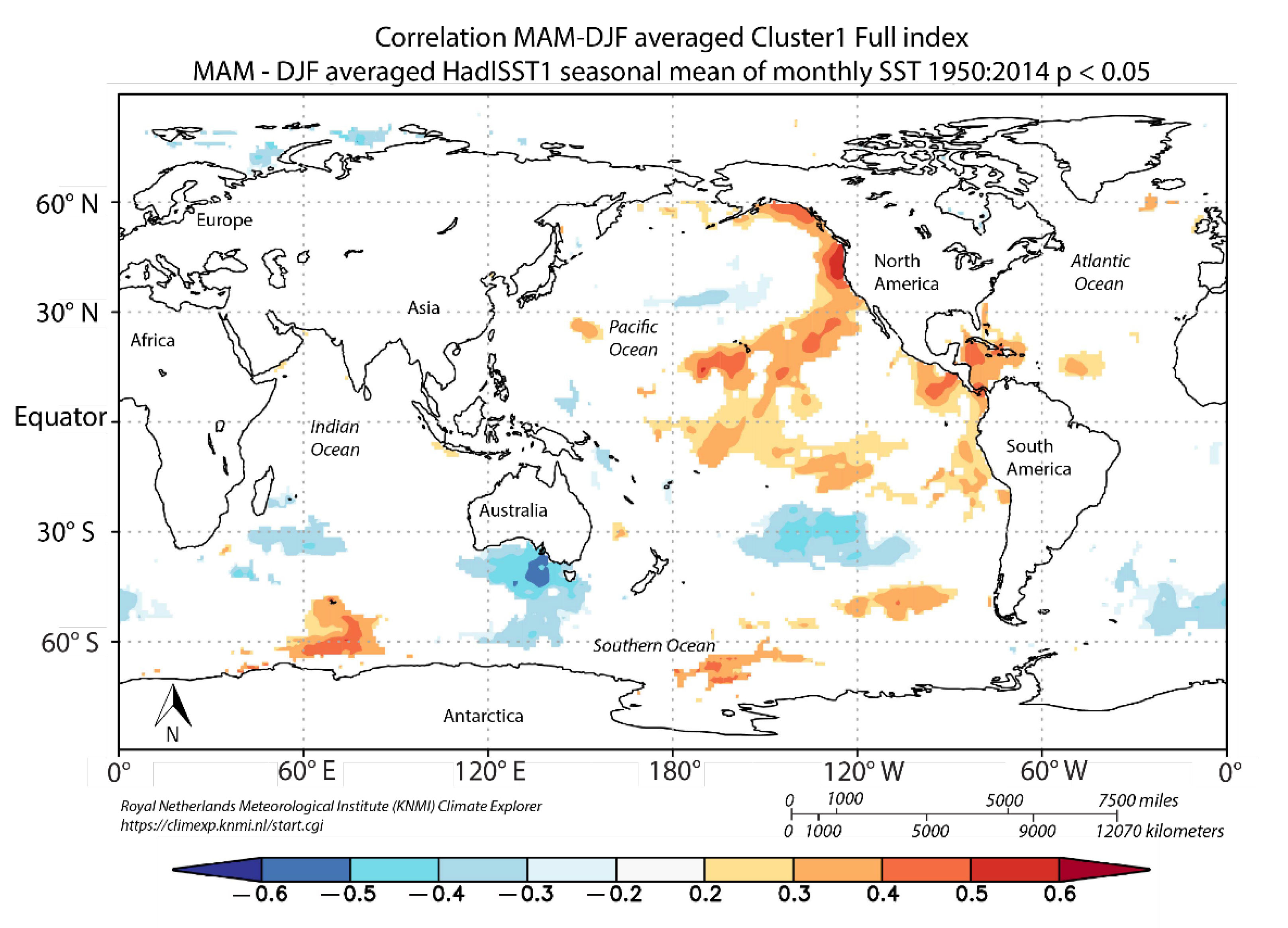
Figure 5.
Spatial correlation of cluster 1 streamflow (converted to Z-scores) with seasonal mean of monthly sea-surface temperature for the period 1950 to 2015. Positive value (warmer color); negative value (cooler color). See Supplementary Materials S1, Figure S1A–E for spatial correlation of clusters 2–5.

Figure 6.
Trends in monthly-mean streamflow in January for the period 1950–2015. Blue dots depict sites with increasing trends, red dots depict sites with decreasing trends, and gray dots depict sites with no significant trends (see Supplementary Materials S1 for Figure S2A–L for months February–December).

Figure 7.
Trends in seasonal mean streamflow in winter for the period 1950–2015. Blue dots indicate sites with increasing trends, red dots indicate sites with decreasing trends, and gray dots depict sites with no significant trends. See Supplementary Materials S1, Figure S3A–D for all seasons.
Figure 7.
Trends in seasonal mean streamflow in winter for the period 1950–2015. Blue dots indicate sites with increasing trends, red dots indicate sites with decreasing trends, and gray dots depict sites with no significant trends. See Supplementary Materials S1, Figure S3A–D for all seasons.

Figure 8.
Trends in the 50th decile of mean annual streamflow for the period 1950–2015. Blue dots indicate sites with increasing trends, red dots indicate sites with decreasing trends, and gray dots depict sites with no significant trends. See Supplementary Materials S1, Figure S4A–K for deciles Q00 to Q100.

Figure 9.
A stacked Quantile-Kendall graph for site no. 79 (USGS station no. 07373000 Big Creek at Pollock, Louisiana) for the: (A) Annual time frame and (B) seasonal time frame. Trend results are plotted at the starting year of the trend analysis period with a significant decreasing trend >2% change in slope per year, shown as a red line, and <2% change in slope per year, shown as a yellow line. Significant increasing trends with a change in slope >2% per year are shown as a blue line, and a change in slope < 2% per year, shown as a green line. The absence of a vertical line (shown as a white line) means that no significant trend was detected for that percentile of flow. HDI-hydrologic disturbance index [29].

Figure 10.
Stacked Quantile-Kendall graphs, annual time frame, for the reference sites in the study area (Mississippi and Louisiana are shown here). See Supplementary Materials S1, Table S1 for other reference sites.
Figure 10.
Stacked Quantile-Kendall graphs, annual time frame, for the reference sites in the study area (Mississippi and Louisiana are shown here). See Supplementary Materials S1, Table S1 for other reference sites.

Figure 11.
Stacked Quantile-Kendall graphs, seasonal time frame, for the 17 reference sites in the study area. (Mississippi and Louisiana are shown here). See Supplementary Materials S1, Table S1 for other reference sites.
Figure 11.
Stacked Quantile-Kendall graphs, seasonal time frame, for the 17 reference sites in the study area. (Mississippi and Louisiana are shown here). See Supplementary Materials S1, Table S1 for other reference sites.

Figure 12.
Spatial variation in the count and the slope of significant trends in the full range of streamflow quantiles for reference sites, annual time frame, for (A) 1950–2015 and (B) 1970–2015.
Figure 12.
Spatial variation in the count and the slope of significant trends in the full range of streamflow quantiles for reference sites, annual time frame, for (A) 1950–2015 and (B) 1970–2015.

Figure 13.
Spatial variation in the number of significant trends in the full range of streamflow quantiles for all sites, annual time frame, for (A) 1950–2015 and (B) 1970–2015.
Figure 13.
Spatial variation in the number of significant trends in the full range of streamflow quantiles for all sites, annual time frame, for (A) 1950–2015 and (B) 1970–2015.

Figure 14.
Trend Departure Index, annual time frame, for the 1950–2015 trend period.


Table 1.
Results of the Mann–Kendall trend test and the Sen’s Slope estimate for the mean Z-score time-series for each cluster of sites. The Sen’s slope estimate is in percent per year. C.I., confidence interval.
Table 1.
Results of the Mann–Kendall trend test and the Sen’s Slope estimate for the mean Z-score time-series for each cluster of sites. The Sen’s slope estimate is in percent per year. C.I., confidence interval.
| Kendall’s Tau | p-Value | Sen’s Slope Estimate | Sen’s Slope C.I. Upper/Lower | |
|---|---|---|---|---|
| Cluster 1 | −0.118 | 0.004 | −0.001 | −0.0022/−0.0004 |
| Cluster 2 | −0.185 | 0.000 | −0.002 | −0.0029/−0.0012 |
| Cluster 3 | −0.105 | 0.010 | −0.002 | −0.0027/−0.0004 |
| Cluster 4 | 0.009 | 0.819 | 0.000 | −0.0009/0.0012 |
| Cluster 5 | 0.085 | 0.038 | 0.001 | 0.0016/0.00004 |
Trend results for which p-value < 0.05 are statistically significant at a 95% confidence level.
Table 2.
Correlation coefficients (ρ) for all clusters with climate indices. PDO, Pacific Decadal Oscillation; AMO, Atlantic Multi-decadal Oscillation; NAO, North Atlantic Oscillation; ENSO, El Nino-Southern Oscillation; PNA, Pacific-North American index.
Table 2.
Correlation coefficients (ρ) for all clusters with climate indices. PDO, Pacific Decadal Oscillation; AMO, Atlantic Multi-decadal Oscillation; NAO, North Atlantic Oscillation; ENSO, El Nino-Southern Oscillation; PNA, Pacific-North American index.
| Climate Index | Cluster 1 | p-Value | Cluster 2 | p-Value | Cluster 3 | p-Value | Cluster 4 | p-Value | Cluster 5 | p-Value |
|---|---|---|---|---|---|---|---|---|---|---|
| PDO | 0.18 | 0.003 | 0.16 | 0.011 | 0.15 | 0.015 | 0.10 | 0.089 | 0.21 | 0.001 |
| AMO | −0.05 | 0.379 | −0.07 | 0.236 | −0.28 | 0.000 | −0.15 | 0.013 | −0.16 | 0.008 |
| NAO | −0.04 | 0.540 | −0.03 | 0.624 | 0.01 | 0.828 | 0.05 | 0.406 | 0.03 | 0.685 |
| ENSO | 0.23 | 0.00 | 0.16 | 0.008 | 0.20 | 0.001 | 0.11 | 0.072 | 0.22 | 0.00 |
| PNA | 0.20 | 0.001 | 0.15 | 0.018 | 0.12 | 0.051 | −0.03 | 0.663 | 0.18 | 0.003 |
Table 3.
Percent of variance explained by each of the climate indices. Time-series of seasonal mean streamflow (converted to Z-scores) for the clusters were regressed with seasonal mean of monthly climate index values. The cluster streamflow time-series were treated as the dependent variable and the climate indices were treated as the independent variable. PDO, Pacific Decadal Oscillation; AMO, Atlantic Multidecadal Oscillation; NAO, North Atlantic Oscillation; ENSO, El Nino-Southern Oscillation; PNA, Pacific-North American index.
| Cluster | PDO | AMO | NAO | ENSO | PNA |
|---|---|---|---|---|---|
| 1 | 3.25 | 0.3 | 0.14 | 5.3 | 3.97 |
| 2 | 2.42 | 0.54 | 0.09 | 2.62 | 2.13 |
| 3 | 2.25 | 7.63 | 0.02 | 4.09 | 1.45 |
| 4 | 1.1 | 2.36 | 0.26 | 1.23 | 0.07 |
| 5 | 4.26 | 2.65 | 0.06 | 4.8 | 3.28 |
Table 4.
Table of monthly mean trend results by the beginning date of the period of analysis through 2015; p-value < 0.05, α = 0.05.
Table 4.
Table of monthly mean trend results by the beginning date of the period of analysis through 2015; p-value < 0.05, α = 0.05.
| 1950 | 1960 | 1970 | |||||||||
| Month | Significant Trends | Increasing Trends | Decreasing Trends | Month | Significant Trends | Increasing Trends | Decreasing Trends | Month | Significant Trends | Increasing Trends | Decreasing Trends |
| January | 25 | 14 | 11 | January | 33 | 5 | 28 | January | 35 | 0 | 35 |
| February | 21 | 7 | 14 | February | 36 | 2 | 34 | February | 35 | 0 | 35 |
| March | 44 | 29 | 15 | March | 38 | 8 | 30 | March | 27 | 2 | 25 |
| April | 29 | 11 | 18 | April | 26 | 3 | 23 | April | 21 | 1 | 20 |
| May | 26 | 4 | 22 | May | 34 | 2 | 32 | May | 42 | 0 | 42 |
| June | 20 | 9 | 11 | June | 34 | 2 | 32 | June | 34 | 0 | 34 |
| July | 29 | 17 | 12 | July | 37 | 9 | 28 | July | 16 | 5 | 11 |
| August | 36 | 23 | 13 | August | 41 | 3 | 38 | August | 57 | 9 | 48 |
| September | 31 | 19 | 12 | September | 34 | 8 | 26 | September | 37 | 5 | 32 |
| October | 33 | 20 | 13 | October | 29 | 5 | 24 | October | 24 | 1 | 23 |
| November | 36 | 23 | 13 | November | 22 | 8 | 14 | November | 19 | 3 | 16 |
| December | 25 | 17 | 8 | December | 17 | 3 | 14 | December | 21 | 1 | 20 |
| 1980 | 1990 | 2000 | |||||||||
| Month | Significant Trends | Increasing Trends | Decreasing Trends | Month | Significant Trends | Increasing Trends | Decreasing Trends | Month | Significant Trends | Increasing Trends | Decreasing Trends |
| January | 12 | 0 | 12 | January | 39 | 0 | 39 | January | 15 | 3 | 12 |
| February | 19 | 0 | 19 | February | 44 | 0 | 44 | February | 21 | 0 | 21 |
| March | 14 | 0 | 14 | March | 42 | 0 | 42 | March | 11 | 0 | 11 |
| April | 7 | 1 | 6 | April | 27 | 0 | 27 | April | 5 | 0 | 5 |
| May | 14 | 0 | 14 | May | 15 | 0 | 15 | May | 4 | 3 | 1 |
| June | 21 | 0 | 21 | June | 24 | 1 | 23 | June | 1 | 0 | 1 |
| July | 12 | 3 | 9 | July | 22 | 4 | 18 | July | 4 | 1 | 3 |
| August | 15 | 2 | 13 | August | 36 | 1 | 35 | August | 10 | 0 | 10 |
| September | 14 | 2 | 12 | September | 26 | 0 | 26 | September | 13 | 0 | 13 |
| October | 16 | 0 | 16 | October | 20 | 0 | 20 | October | 7 | 0 | 7 |
| November | 24 | 0 | 24 | November | 31 | 0 | 31 | November | 14 | 0 | 14 |
| December | 18 | 0 | 18 | December | 30 | 0 | 30 | December | 24 | 0 | 24 |
Table 5.
Trend results in seasonal mean streamflow for each decade starting in 1950 through 2015; p-value < 0.05, α = 0.05.
Table 5.
Trend results in seasonal mean streamflow for each decade starting in 1950 through 2015; p-value < 0.05, α = 0.05.
| 1950 | 1960 | 1970 | |||||||||
| Season | Significant Trends | Increasing Trends | Decreasing Trends | Season | Significant Trends | Increasing Trends | Decreasing Trends | Season | Significant Trends | Increasing Trends | Decreasing Trends |
| Spring | 25 | 9 | 16 | Spring | 34 | 3 | 31 | Spring | 29 | 1 | 28 |
| Summer | 23 | 12 | 11 | Summer | 36 | 7 | 29 | Summer | 41 | 2 | 39 |
| Fall | 48 | 30 | 18 | Fall | 36 | 11 | 25 | Fall | 27 | 2 | 25 |
| Winter | 22 | 11 | 11 | Winter | 32 | 3 | 29 | Winter | 34 | 1 | 33 |
| 1980 | 1990 | 2000 | |||||||||
| Season | Significant Trends | Increasing Trends | Decreasing Trends | Season | Significant Trends | Increasing Trends | Decreasing Trends | Season | Significant Trends | Increasing Trends | Decreasing Trends |
| Spring | 6 | 0 | 6 | Spring | 29 | 0 | 29 | Spring | 2 | 0 | 2 |
| Summer | 14 | 1 | 13 | Summer | 32 | 1 | 31 | Summer | 3 | 0 | 3 |
| Fall | 17 | 1 | 16 | Fall | 28 | 0 | 28 | Fall | 15 | 0 | 15 |
| Winter | 16 | 0 | 16 | Winter | 39 | 0 | 39 | Winter | 20 | 1 | 19 |
Table 6.
Trend results in decile streamflow starting in each decade from 1950 through 2015. p-value < 0.05, α = 0.05; Q00: low flow, Q10: 10th decile, Q20: 20th decile, Q30: 30th decile, Q40: 40th decile, Q50: 50th decile, Q60: 60th decile, Q70: 70th decile, Q80: 80th decile, Q90: 90th decile, Q100: high flow.
| 1950 | 1960 | 1970 | |||||||||
| Decile | Significant Trends | Increasing Trends | Decreasing Trends | Decile | Significant Trends | Increasing Trends | Decreasing Trends | Decile | Significant Trends | Increasing Trends | Decreasing Trends |
| Q00 | 70 | 35 | 35 | Q00 | 77 | 28 | 49 | Q00 | 82 | 16 | 66 |
| Q10 | 61 | 32 | 29 | Q10 | 72 | 24 | 48 | Q10 | 78 | 13 | 65 |
| Q20 | 49 | 29 | 20 | Q20 | 63 | 20 | 43 | Q20 | 79 | 10 | 69 |
| Q30 | 48 | 31 | 17 | Q30 | 56 | 16 | 40 | Q30 | 66 | 6 | 60 |
| Q40 | 45 | 29 | 16 | Q40 | 49 | 12 | 37 | Q40 | 68 | 5 | 63 |
| Q50 | 42 | 28 | 14 | Q50 | 44 | 10 | 34 | Q50 | 60 | 5 | 55 |
| Q60 | 31 | 18 | 13 | Q60 | 38 | 7 | 31 | Q60 | 55 | 3 | 52 |
| Q70 | 39 | 27 | 12 | Q70 | 36 | 7 | 29 | Q70 | 50 | 2 | 48 |
| Q80 | 27 | 16 | 11 | Q80 | 29 | 5 | 24 | Q80 | 41 | 1 | 40 |
| Q90 | 22 | 13 | 9 | Q90 | 24 | 3 | 21 | Q90 | 27 | 1 | 26 |
| Q100 | 31 | 9 | 22 | Q100 | 28 | 3 | 25 | Q100 | 21 | 2 | 19 |
| 1980 | 1990 | 2000 | |||||||||
| Decile | Significant Trends | Increasing Trends | Decreasing Trends | Decile | Significant Trends | Increasing Trends | Decreasing Trends | Decile | Significant Trends | Increasing Trends | Decreasing Trends |
| Q00 | 50 | 8 | 42 | Q00 | 51 | 5 | 46 | Q00 | 21 | 0 | 21 |
| Q10 | 37 | 6 | 31 | Q10 | 66 | 4 | 62 | Q10 | 22 | 0 | 22 |
| Q20 | 39 | 4 | 35 | Q20 | 61 | 1 | 60 | Q20 | 24 | 0 | 24 |
| Q30 | 35 | 1 | 34 | Q30 | 59 | 1 | 58 | Q30 | 26 | 0 | 26 |
| Q40 | 34 | 2 | 32 | Q40 | 64 | 0 | 64 | Q40 | 26 | 0 | 26 |
| Q50 | 28 | 2 | 26 | Q50 | 63 | 0 | 63 | Q50 | 24 | 0 | 24 |
| Q60 | 26 | 2 | 24 | Q60 | 60 | 0 | 60 | Q60 | 17 | 0 | 17 |
| Q70 | 19 | 1 | 18 | Q70 | 54 | 0 | 54 | Q70 | 12 | 2 | 10 |
| Q80 | 14 | 1 | 13 | Q80 | 46 | 1 | 45 | Q80 | 9 | 3 | 6 |
| Q90 | 8 | 1 | 7 | Q90 | 25 | 1 | 24 | Q90 | 4 | 0 | 4 |
| Q100 | 6 | 1 | 5 | Q100 | 17 | 0 | 17 | Q100 | 3 | 1 | 2 |
Table 7.
Summary by the cluster of trends and the Trend Departure Index (TDI) for the period 1970–2015, annual time frame for all sites. TDI varies from 0 to 1; a TDI of 0 indicates the trend results for the site are identical to the reference site.
Table 7.
Summary by the cluster of trends and the Trend Departure Index (TDI) for the period 1970–2015, annual time frame for all sites. TDI varies from 0 to 1; a TDI of 0 indicates the trend results for the site are identical to the reference site.
| Reference Sites | |||||||||
| Increasing Trends | Decreasing Trends | ||||||||
| Count of quantiles with trends | Count of quantile with trends | ||||||||
| Cluster | Number of sites | Average per site | Standard deviation | Average slope, in percent | Average per site | Standard deviation | Average slope, in percent | ||
| 1 | --a | --a | --a | --a | --a | --a | --a | ||
| 2 | 1 | 0 | --b | --c | 0 | --b | --c | ||
| 3 | 2 | 0 | 0 | --c | 17 | 6 | −4.07 | ||
| 4 | 3 | 0 | 0 | --c | 150 | 95 | −1.11 | ||
| 5 | 5 | 0 | 0 | --c | 190 | 139 | −3.01 | ||
| All | 17 | 0 | 0 | --c | 137 | 115 | −2.07 | ||
| All Sites (excluding spatially dependent sites d) | |||||||||
| Increasing trends | Decreasing trends | Trend Departure Index | |||||||
| Count of quantiles with trends | Count of quantile with trends | ||||||||
| Cluster | Number of sites | Average per site | Standard deviation | Average slope, in percent | Average per site | Standard deviation | Average slope, in percent | Average | Standard deviation |
| 1 | 6 | 3 | 6 | 1 | 18 | 27 | −2.71 | 0.06 | 0.07 |
| 2 | 3 | 0 | 0 | --c | 32 | 52 | −3.10 | 0.09 | 0.14 |
| 3 | 8 | 0 | 0 | --c | 148 | 143 | −2.18 | 0.38 | 0.38 |
| 4 | 49 | 0 | 0 | --c | 130 | 126 | −1.23 | 0.37 | 0.28 |
| 5 | 51 | 15 | 45 | 2.38 | 72 | 118 | −2.79 | 0.68 | 0.41 |
| All | 117 | 7 | 31 | 2.24 | 97 | 123 | −1.91 | 0.48 | 0.39 |
a Cluster 1 does not include a reference site; for the purpose of calculating TDI a reference site from Cluster 2 was associated with sites in Cluster 1; b Standard deviation is not calculated for n = 1; c Mean slope not reported because there were no significant trends; d Results for pairs of sites located close together on the same flow path are not independent; one site from each pair is excluded for this summary.
Publisher’s Note: MDPI stays neutral with regard to jurisdictional claims in published maps and institutional affiliations. |
© 2020 by the authors. Licensee MDPI, Basel, Switzerland. This article is an open access article distributed under the terms and conditions of the Creative Commons Attribution (CC BY) license (http://creativecommons.org/licenses/by/4.0/).
Share and Cite
MDPI and ACS Style
Rodgers, K.; Roland, V.; Hoos, A.; Crowley-Ornelas, E.; Knight, R. An Analysis of Streamflow Trends in the Southern and Southeastern US from 1950–2015. Water 2020, 12, 3345. https://doi.org/10.3390/w12123345
AMA Style
Rodgers K, Roland V, Hoos A, Crowley-Ornelas E, Knight R. An Analysis of Streamflow Trends in the Southern and Southeastern US from 1950–2015. Water. 2020; 12(12):3345. https://doi.org/10.3390/w12123345
Chicago/Turabian StyleRodgers, Kirk, Victor Roland, Anne Hoos, Elena Crowley-Ornelas, and Rodney Knight. 2020. "An Analysis of Streamflow Trends in the Southern and Southeastern US from 1950–2015" Water 12, no. 12: 3345. https://doi.org/10.3390/w12123345
Note that from the first issue of 2016, this journal uses article numbers instead of page numbers. See further details here.