The Role of Water Supply Development in the Earth System

Abstract

The ANEMI model is an integrated assessment model of global change that emphasizes the role of water resources. Securing water resources for the future is a key issue of global change and ties into global systems of population growth, climate change carbon cycle, hydrologic cycle, economy, energy production, land use and pollution generation. The focus of the presented work is on the development of global water supplies necessary to keep pace with a growing population and global economy. With the structure of the ANEMI model, a series of experiments are conducted in order to assess: (i) the current role of water supply in the global Earth system; (ii) the level of water stress that can be expected in the future; and (iii) what are the potential effects of water quality on global surface water supply and the distribution of water supply types. The results of model simulations show that surface water resources were sufficient to meet the water demand and water quality is not shown to be a significant factor for the development of surface water supplies. Due to globally aggregated scale, these impacts are averaged and likely understated.

1. Introduction

Human impacts on the environment at global scales are being realized through our ability to alter atmospheric concentrations of greenhouse gases and consequently global climate, creating the need to consider environmental problems and their interactions with the Earth as a highly integrated system. The Earth system is composed of biological, physical, chemical and human elements that form a network of feedbacks through their interconnections [1]. The concept of global change becomes increasingly important as the components of the Earth system such as population growth and migrations, economic productivity, climate, food production and hydrology are interlinked through dynamic non-linear feedback processes [2]. Within this system, changes in one component inevitably lead to changes in another. This is why global change research focusses on interactions between components of the Earth system as a whole, as opposed to only those of climate [1,3].

The main focus of the presented work is to answer the following questions through the implementation of the global model of the Earth system: (i) What level of water stress can be expected in the future?; (ii) Can alternative water supplies help to alleviate future water stress?; and (iii) What are the potential effects of water quality on global surface water supply and the distribution of water supply types?

1.1. Water in the Earth System

Water can be considered one of, if not the most, important drivers for human life as well as social and economic development [4]. Water resources provide for the most basic human needs of drinking and sanitation, while allowing for irrigated agriculture to take place and industrial activities such as thermal power generation, mining and manufacturing. Therefore, the use of, management and availability of water resources plays a crucial role in the progression of global changes in the Earth system as without it, societies cannot function.

A growing global population and its needs has put stress on water resources in many regions around the World. This problem will continue to grow as the population is projected (a) to increase 42% by the year 2100 to 10.9 billion people [5]; and (b) migrate–1 billion people may become climate refugees by 2050 [6]. The demand for water increases not only with the population but also with the consumption of water on a per capita basis. Alcamo et al. in Reference [7], show that countries with higher gross domestic product (GDP) per capita generally have higher water usage in the domestic sector and follow a type of S-curve, while in the industrial sector, water usage decreases exponentially to an equilibrium value. Therefore, as countries continue to develop economically the water usage patterns will change. By continuing with the current trends in global population, economics and technological change, water demand will continue to increase in most developing countries due increased domestic water usage as well as agricultural production. In developed countries domestic and industrial demands saturate and the expansion of irrigated land stagnates [8].

Water stress is often defined as the ratio of water withdrawals to the available water resources in a region. The hydrologic cycle along with changes made to it through anthropogenic means dictates the amount of water resources that are available for use. Although natural variability in weather patterns can determine if a region will experience wet or dry seasons, human influence on hydrologic cycles such as the construction and operation of dams and reservoirs, water diversions and water withdrawals redistribute the water availability in time and space. Climate change is expected to alter the spatial and temporal distribution of water resources on top of what is observed naturally and through direct human influence [9]. Increased global temperature through the greenhouse effect is expected to intensify the hydrologic cycle, leading to higher evapotranspiration rates, more frequent and heavier storms and faster flowing rivers, along with the potential for longer periods of drought. Because of this, there exists the potential for the availability of water resources to be changed for better or worse in different areas of the world [10].

Water resources may be available in a given point in time and space; however, the quality of that water can sometimes dictate whether or not it is available for a certain type of use. For example, according to a national report from the US Environmental Protection Agency almost half of rivers and streams across the US are categorized as with “poor biological condition” as a result of nutrient and sediment pollution. The condition of the rivers and streams are deemed unfit for fishing and recreational use [11]. In China, the situation is even worse with more than 70 percent of rivers and lakes being polluted and almost half may contain water unfit for human consumption or contact [12].

Degrading water quality over time has been shown to cause maintenance and treatment issues in drinking water treatment plants. There is evidence that increases in dissolved organic matter can lead to fouling and blocking membranes and filters, cause harmful disinfection by-products, facilitate biological re-growth in distribution systems and transport pesticides, pharmaceuticals and heavy metal into treatment systems [13]. There are a number of studies that highlight the relationship between the water quality and the water treatment, which can lead to water supplies inadequate for human consumption. Changes in water quality on a global scale could be a significant concern for our ability to maintain clean and sufficient water supplies.

Solutions to ensuring freshwater security vary from managing water demands and more accurately modelling water resource availability (surface and ground water), to technological solutions such as desalination and water reuse. Desalination involves the use of thermal evaporation or membrane separation technology to remove dissolved solids that are present in saline water sources. Both methods are highly energy intensive and can be costly when compared to traditional water supplies. Currently, there are approximately 16 thousand operational desalination plants around the World producing over 95 million m³/day of desalinated water for human use [14]. The cost associated with producing this type of water supply is estimated to be between 0.45 to 2.51 $/m³, which is still 2 to 3 times higher than conventional water supply but it is rapidly decreasing (approximately a factor of 10 since the 1960s [15].

Water reuse technologies involve the treatment of waste waters from a variety of different uses such as agricultural, municipal and industrial. The level of treatment necessary is dependent on the composition of waste waters being treated as well as the type of reuse that is under consideration. For non-potable reuse, wastewater is treated to a lower standard while potable uses require more advanced treatment methods capable of removing emerging pathogens, endocrine disrupting chemicals and pharmaceuticals [16]. Treatment options vary from simple low-energy solutions such as lagoons which allow wastewater to filter through media, to high-energy advanced treatment plants employing activated sludge treatment along with different levels of disinfection ranging from ultra-violet to membrane filtration.

1.2. Integrated Assessment Modelling

Water resources management in the context of global change involves many different disciplines ranging from climate science, economics, hydrology, biology, engineering, governance, agriculture and social sciences as outlined above. In order to address the problem of dealing with future water stress, these disciplines must be put together in a comprehensive framework. This will allow decision makers to explore policy options that consider the Earth system as a whole.

Assessment of various aspects of global change often requires the use of models from different domains and new tools and modelling paradigms to analyze complex interactions in the Earth system at a variety of spatial and temporal scales. The concept of integrated assessment (IA) has been defined as an interdisciplinary process of bringing together knowledge from different disciplines, adding value in contrast to a single disciplinary approach in order to provide information to decision and policy makers [17]. It is performed to bring about understanding of an issue regardless of the discipline.

Tol and Vellinga in Reference [18] describe the process of IA in a set of stages. The first stage involves structuring the problem that is to be assessed. The boundary of the problem must be defined in a way that encompasses all the important components of the problem, as well as components that may become important to the problem under different conditions or over time. Stage 2 involves the use of participatory and modelling methods for assessment to engage stakeholders that play a role in the problem at hand.

The integrated assessment modelling (IAM) approach involves the coupling of disciplinary models. There are many different methods that can be used to form a model for integrated assessment. Connections between disciplinary models can be made statically (output of one model is first obtained then given as input to another) or dynamically (both models running at the same time). The latter of which, is the only way that feedback loops can be created and studied. Dynamic connections can be made by using a computer program to facilitate the exchange of information while the models are running or both models can be combined into the same computer code [18].

1.3. System Dynamics Simulation for Integrated Assessment

The field of system dynamics focusses specifically on analyzing the dynamic nature of systems that are composed of feedback loops. Therefore, the use of system dynamics is ideal for the construction of integrated assessment models of global change. The system dynamics modelling process involves the use of causal loop diagramming to map out the feedback loops that are driving system behavior. This is effectively describing the boundary of the problem as well as the components that are responsible for reproducing it. System dynamics simulation builds from the conceptual models developed through systems thinking by adding structure to them. The addition of stocks or state variables and the flows that affect them, takes the system from a conceptual model to a mathematical model through stock and flow diagramming. Stock and flow diagrams illustrate the configuration of stocks and flows which is essentially a visual representation of a system of first order differential equations. Most, if not all, IAMs can be represented in this way from a high level. Therefore, the system dynamics simulation approach is ideal for the construction of IAMs and provides a formalized way for creating feedback loops between disciplinary models of global change.

1.4. The Role of Water Supply Development in the Earth System

The ANEMI model [19,20] is an integrated assessment model of global change that emphasizes the role of water resources. The model is based on the principles of system dynamics simulation in order to analyze changes in the Earth system using feedback processes. Securing water resources for the future is a key issue of global change and ties into global systems of population growth, climate change carbon cycle, hydrologic cycle, economy, energy production, land use and pollution generation.

The main contribution of the presented work is the development of global water supplies necessary to keep pace with a growing population and global economy using an integrated feedback-based approach. With the structure of the ANEMI model, a series of experiments are conducted in order to assess: (i) the current role of water supply in the global Earth system; (ii) the level of water stress that can be expected in the future; and (iii) what are the potential effects of water quality on global surface water supply and the distribution of water supply types.

Evaluation of the model performance demonstrates that the model can reproduce historical trends related to global change within the Earth system. The experimental results show that investment in alternative water supplies on a global scale should be made in advance of conventional water supply depletion, as time delays may result in prolonged increases in global water stress. It was also found that the role of technological change was a greater factor for meeting future food production requirements than the effect of a changing climate. The impact of water quality degradation and the depletion of available water resource on water supply development, was found to be understated when studied on the global scale. It is recommended that the water supply development system developed in this work be extended to a finer spatial scale where the effects of water depletion and water quality degradation can be more thoroughly examined.

2. Overview of the ANEMI3 Model of Global Change

This chapter presents the ANEMI model, which is currently in version 3 [19,20], built upon the first two iterations of ANEMI [21,22]. The model shares the same system dynamics simulation paradigm that was used in the previous iterations of ANEMI, in that feedbacks and delays are used to drive system behavior. ANEMI3 is a type of integrated assessment model that describes the state of and interactions between model sub-systems that compose the Earth system. The main sub-systems or ‘sectors’ used are that of the climate system, carbon, nutrient and hydrologic cycles, population dynamics, land use, food production, sea level rise, energy production, global economy, persistent pollution, water demand and water supply development.

Each individual sector in the model describes the relevant feedbacks that drive the state variables in the sector. Connections between sectors form intersectoral feedbacks responsible for the functioning of the Earth system. It is the intersectoral feedbacks that allow us to represent feedbacks that drive global changes in the Earth system. Feedbacks driving global change are now evident, while is expected that negative feedbacks acting on population and economic growth may be more evident in the future. From a system dynamics perspective, effective policymaking should be based on addressing the feedback structure of a system, not only on modifying the system parameters. This viewpoint is what makes the ANEMI3 model unique and useful since in the current time global modelling is becoming progressively more complex [23].

The boundary of the model is defined by the problem that is being explored. In this case, we are modelling the role of water resources in various aspects of global change. Therefore, the spatial scale of the model is mainly one that is global. In some sectors, the stocks are disaggregated to capture material flows on a sub-global scale but not at a level that is location specific. This spatial scale limits the level of detail that can be used to describe the flows that act to change the model stocks, however it allows us to effectively analyze feedbacks between water resources and other model sectors on a global scale.

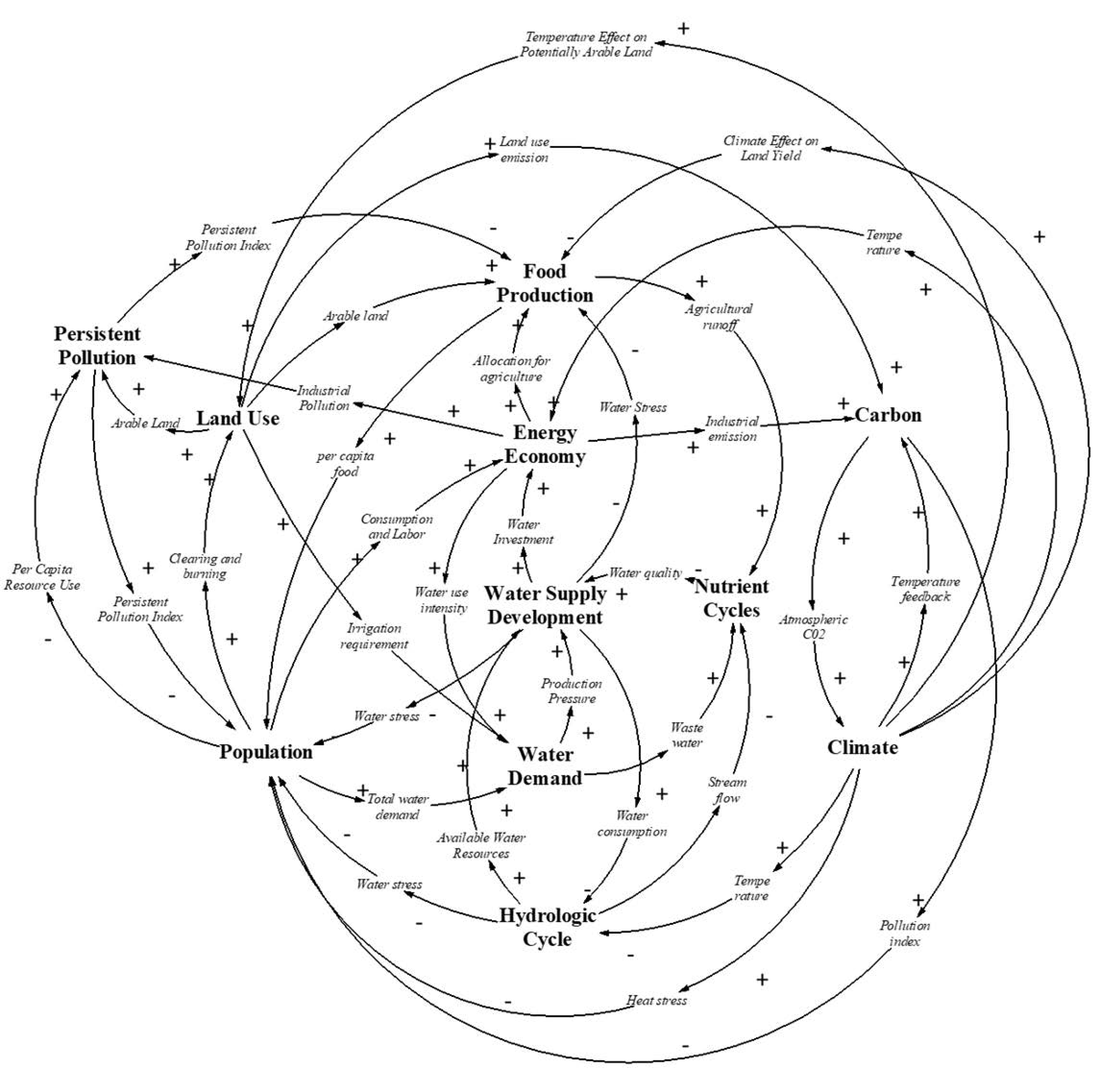
The highly endogenous structure and coupling of sub-systems in the ANEMI3 model are part of its novelty in the realm of integrated assessment modelling. Because of this, feedback processes are responsible for the behavior that is exhibited in model runs. The model sectors that comprise the ANEMI3 model are that of the climate system, carbon, nutrient and hydrologic cycles, population dynamics, land use, food production, sea level rise, energy production, global economy, persistent pollution, water demand and water supply development as shown in Figure 1. The model includes over 2000 variables and 700 equations. Presentation in Figure 1 is focused on illustrating the high-level model sectoral structure and relationships. Feedback loops between sectors or intersectoral feedback loops are responsible for global change in this Earth system. Intersectoral feedbacks in the ANEMI3 model allow for the representation of various aspects of global change. In the Figure 1 diagram alone there is a total of 89 possible intersectoral feedback loops. The size of the feedback loops range from 2 to 9 sectors included out of the 10 that are shown. An example is that of a growing global economy, which drives energy production and industrial growth, thereby resulting in more greenhouse gas emissions and climate change. This in turn results in negative feedbacks on economic growth through climate damages, which can represent economic damages because of land and structures lost to coastal flooding, for example. Creating a causal loop diagram from these connections between model sectors allows us to view the feedbacks that are created by combining model sectors in this way.

The main difference between ANEMI1, ANEMI2 and ANEMI3 is addition of intersectoral feedback loops used to (a) analyze water supply development within the Earth system, (b) include of water quality degradation and its impact on the development of surface water supplies and (c) assess of global scale feedback related to water supply development. These main modifications are introduced to represent the dynamics of global change at the global scale with an emphasis on the development of water supplies.

The ANEMI model is developed using Vensim (https://vensim.com/ last accessed 20 November 2020) system dynamics simulation software. The current model code is archived using Zenodo (https:doi.org/10.5281/zenodo.4025424) and details on how to run the model, modify inputs and view the outputs in graphical or tabular formats are provided in the repository and discussed in Reference [19]. Work presented in this paper is building on the work and data from previous versions of the model [15,16,19].

2.1. Integrated Assessment of Global Water Resources

The new water supply sector in ANEMI3 was developed by incorporating water supply as a new production sector within the newly added energy-economy sector [19,20,23]. This has been achieved by adding capital stocks to produce water supply in the form of surface, ground, wastewater reclamation and desalination water sources.

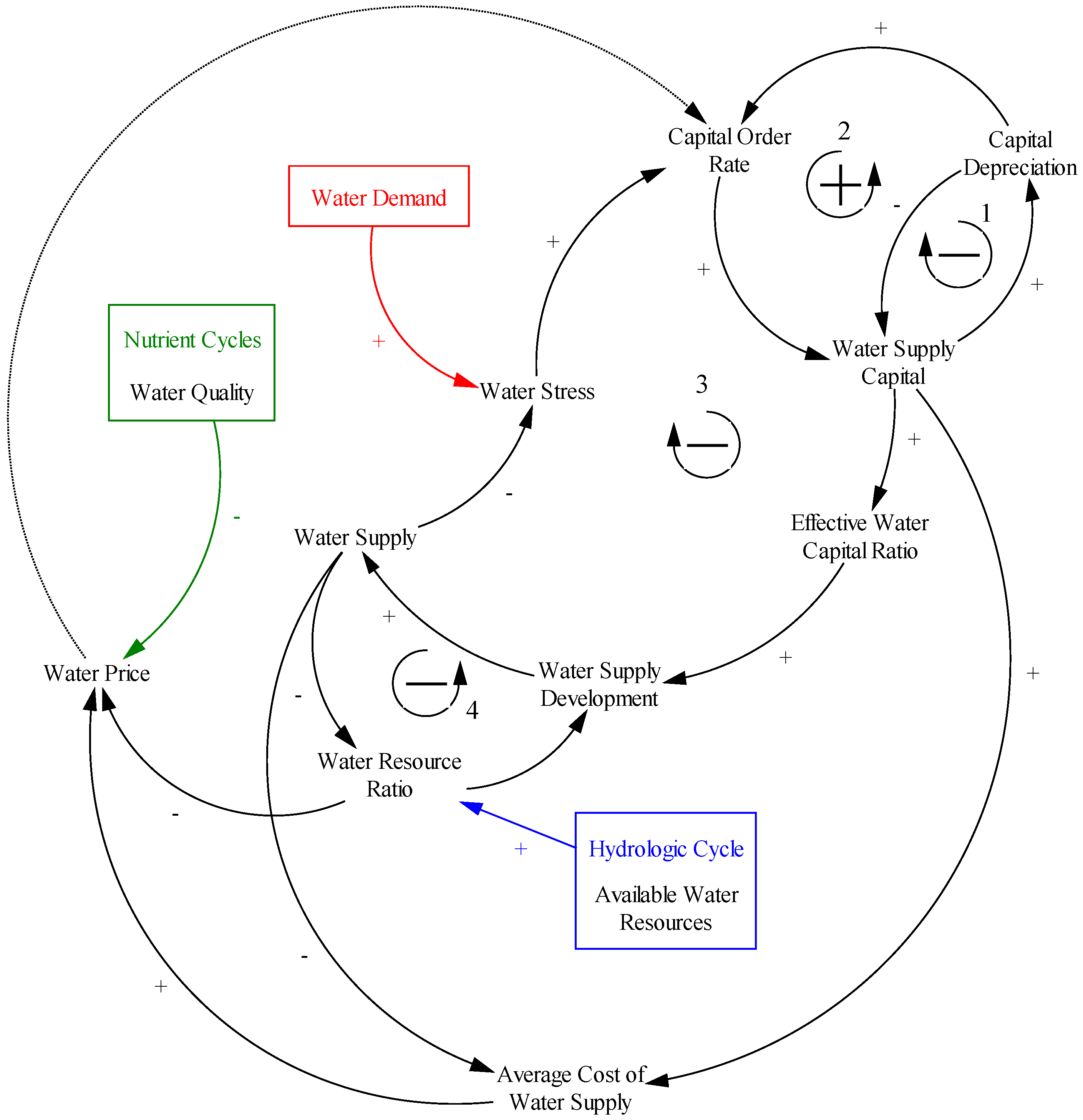
As available water resources become depleted, the water supply is reduced for the same input intensity. This means that more effort is required to produce the same rate of water supply, which also makes a given type of water supply that is depleted more expensive. For example, when the groundwater elevation decreases from over abstraction, more pumping energy is required to extract the same amount of water resource. The effect of saturation is also included in this relationship, assuming the best or most cost-effective sites are used first for water supply infrastructures. An example of which could include the construction of additional reservoirs, source water intakes, of groundwater wells in areas that are less suitable or cost effective than those that were previously constructed.

The dotted causal link from water price to the capital order rate in Figure 2 indicates a connection that is neither positive nor negative. Instead, this link is used to determine the amount of investment that is made in the capital stocks of the different supply types (surface, ground, wastewater reclamation and desalination water sources). Inputs from the nutrient cycle, hydrologic cycle and water demand sectors are used to define the water price, water stress and water resource ratio variables respectively in the water supply development sector.

2.2. Mathematical Formulation of Water Supply Development Sector

Water resources, $R_i$ are used in the production of water supplies, where the subscript $i$, denotes the type of water supplies for which the water resources are being used.

$$R_{sw}=S_r\times TRF-URW\times WPF \left[{\mathrm{km}}^3/\mathrm{y}\right]$$

(1)

$$R_{gw}=Q_{perc}-Q_{discharge} \left[{\mathrm{km}}^3/\mathrm{y}\right]$$

(2)

$$R_{ww}=TDW+TIW \left[{\mathrm{km}}^3/\mathrm{y}\right]$$

(3)

$$R_{ds}=Oceans \left[{\mathrm{km}}^3\right],$$

(4)

where $R_{sw}$ = Surface water resources $\left[{\mathrm{km}}^3/\mathrm{y}\right]$; $R_{gw}$ = Groundwater resources $\left[{\mathrm{km}}^3/\mathrm{y}\right]$; $R_{ww}$ = Wastewater resources $\left[{\mathrm{km}}^3/\mathrm{y}\right]$; $R_{ds}$ = Desalination water resources; $S_r$ = Stable and reusable runoff fraction; TRF = Total renewable flow $\left[{\mathrm{km}}^3/\mathrm{y}\right]$; WPF = Wastewater pollution factor; $Q_{perc}$ = Percolation to groundwater $\left[{\mathrm{km}}^3/\mathrm{y}\right]$; $Q_{discahrge}$ = Groundwater discharge $\left[{\mathrm{km}}^3/\mathrm{y}\right]$; TDW = Treated domestic wastewater $\left[{\mathrm{km}}^3/\mathrm{y}\right]$; TIW = Treated industrial wastewater $\left[{\mathrm{km}}^3/\mathrm{y}\right]$; URW = Untreated Returnable Waters $\left[{\mathrm{km}}^3/\mathrm{y}\right]$.

The amount of water resources available for the development of water supplies is dependent on the hydrologic cycle, water demand and water quality sectors of the model. In the case of surface water, the stable and reusable portion of runoff is taken from the total renewable streamflow and is adjusted for untreated wastewater discharge. The adjustment for wastewater discharge is based on [24] which estimates that for every cubic meter of contaminated wastewater discharged into water bodies and streams, makes unsuitable 8–10 cubic meters of fresh water. The difference in groundwater percolation and discharge is used for the consideration of groundwater resources as this refers to renewable groundwater. Only renewable groundwater resources are considered for the global scale. The inclusion of non-renewable or fossil groundwater resources should be considered at the regional scale. For the potential reuse of wastewater, industrial and domestic wastewaters are considered. Although the reuse of wastewater is highly dependent on the type of wastewater and the use for which it is being treated, it is considered here as a supplementary type of water supply in the case of groundwater and surface water depletion. Water resources used for desalination are considered primarily from the ocean stock in the hydrologic cycle. This results in a virtually limitless supply; however, it is very energy intensive resulting in a high effective input intensity thereby limiting production.

The concept of resource depletion in energy production is also applicable to water supply development. For example, in the case of surface water and groundwater resources, depleted water resources will mean less suitable locations for water extraction and treatment plants. This might mean that source waters could be further from where the water is being used, thus increasing distribution costs. Pumping costs could also be increased by using deeper aquifers or surface water supplies that have a greater difference in elevation from their point of use. Water resource depletion factors into the water supply development process in much the same way as energy production, however there is one key difference. The depletion effect for energy production is based on the ratio of current energy resources remaining to the initial amount. In contrast, water resources are renewable to varying degrees. Therefore, simply taking the ratio of the available water resources to the initial water resources is insufficient. Here, the ratio of available water resources to the current production level is used. In order to accomplish this structure, water production was changed to a stock variable to avoid creating an indeterminate system (introduction of a new negative feedback by making water production a function of itself).

$$W{S}_i=\int W{S}_{i,0}{\left({\alpha }_{w_i}{\left(\frac{W{S}_i}{A{W}_i}\right)}^{{\rho }_w{}_i}+\left(1-{\alpha }_{w_i}\right)EWI{I}_i^{{\rho }_w{}_i}\right)}^{\frac{1}{{\rho }_{w_i}}}\times dt\left[{\mathrm{km}}^3/\mathrm{y}\right],$$

(5)

where $W{S}_i$ = Water supply from water resource i $\left[{\mathrm{km}}^3/\mathrm{y}\right]$; $W{S}_{i,0}$ = Initial water production $\left[{\mathrm{km}}^3/\mathrm{y}\right]$; $A{W}_i$ = Available water resource remaining $\left[{\mathrm{km}}^3/\mathrm{y}\right]$; $EWI{I}_i$ = Effective water input intensity; ${\alpha }_w{}_i$ = Water resource share; ${\rho }_w{}_i$ = Resource substitution coefficient.

In the case of surface water, the available water resources are a rate (runoff minus water quality depletion effects) rather than a stock that can be depleted over time. If production equals this rate, then there is no more surface water that can be utilized at this time step. For wastewater reuse if the rate of reuse is equal to that of the amount of treated wastewater, then no more wastewater can be reused unless wastewater treatment percentage increases.

In the energy capital sub-system of the energy-economy sector, the desired energy capital for each source is determined by the perceived return on investment and the production pressure defined as the ratio of the energy order rate or demand to energy production for each source [19,20]. In the case of water supply, the term for perceived return on investment is removed, thereby making the primary drive for new water supply capital based on production pressure, which resembles the definition of water stress (withdrawal or demand to availability ratio). This value is multiplied by the current water capital stocks to obtain the desired water capital stocks,

$$DK{W}_i=K{W}_i\times \frac{W_d{}_i}{W{S}_i}\left[\$\right],$$

(6)

where $DK{W}_i$. = Desired water capital for water source i $\left[{\mathrm{km}}^3/\mathrm{y}\right]$; $W_{d_i}$ = Demand for water supply i $\left[{\mathrm{km}}^3/\mathrm{y}\right]$; $W{S}_i$ = Water supply from water source i $\left[{\mathrm{km}}^3/\mathrm{y}\right]$.

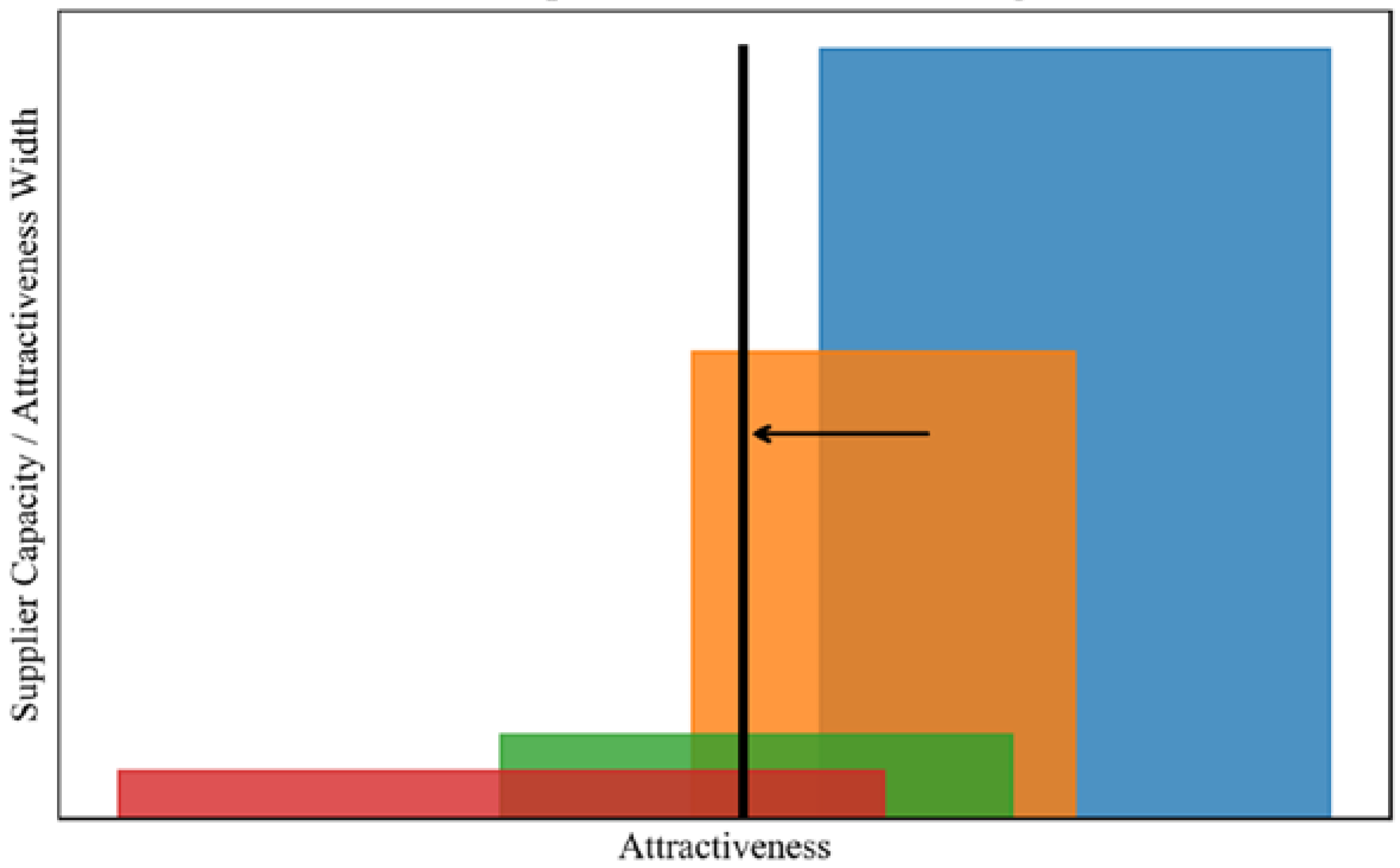
Where $i$ denotes the type of water supply for which desired water capital is being determined. In order to obtain the demand for water supply from each source, Wood’s algorithm [21] is used to allocate the total water demand (sum of domestic, industrial and agricultural water demand) to each supplier. The geometric illustration of Wood’s algorithm is shown in Figure 3, where each rectangle represents a different supplier (blue-surface, orange-ground, green-wastewater reclamation and red-desalination water supplies). The area of each rectangle represents the capacity for a given supplier to fulfil the demand for a product, while the position and width of each rectangle is based on the “attractiveness” value and “width” parameters respectively. Here, the inverse water supply price is used to represent the attractiveness value and the area of each rectangle would be the water supply capacity for a given supply type. The total water demand is allocated to each supplier by the black line in Figure 3 which moves from right to left until the area to the right of the line fulfils the demand. The area of each rectangle that lies on the right of the black line represents the level of demand satisfied by each supplier, therefore a water supply type with a high price would be placed farther to the left on the attractiveness scale and would receive less of the total water demand.

The inverse water supply price was chosen as the main driver for changes in supplier attractiveness as this will vary with technological improvements, depletion, saturation and water quality in the case of surface water supply. This formulation encapsulates the effects of global changes in technology, water resource availability and water quality on the allocation of capital investments in different types of water supply. The width factor determines how this allocation is distributed to suppliers which are not necessarily the cheapest option. For example, on the global scale, although the use of surface water supplies is likely the most cost-effective option in many regions, groundwater, water reuse and desalination supplies are all being used simultaneously.

The concept of endogenous technological change applied to energy production [19,20] has analogies to water supply development. In the case of surface water and groundwater supplies, it is assumed that pumping, distribution and treatment technologies will remain largely the same but will show some improvement over time. However, alternative water supplies such as wastewater reuse and desalination are likely to see vast improvements in the near future. Factoring technological change into the water supply development process is what will help make alternative water supplies more feasible in the future, along with depletion and saturation of conventional water supplies.

A unique attribute of water resources when considering water supply development is water quality. Degraded water quality can impact the functioning of water treatment facilities as well as maintenance costs and the necessary configuration of unit processes [22]. This may also influence the ability to secure adequate source waters for extraction of water resources in the future as a result of pollution and climate change. This could negatively impact production of conventional water supplies by increasing the cost of implementing new capital as well as variable inputs needed for treatment and distribution including energy, chemicals and labor.

In ANEMI3, nutrient concentrations in surface waters are used as an indicator of water quality on a global scale [19,20,22]. Wastewater and agricultural inputs are used as the main contributors to water quality degradation and changes in the levels of nutrients in the form of total nitrogen and phosphorus are used as indicators of water quality from the nutrient cycle sector of the model. The ratio of current to initial nutrient concentrations for surface water resources is used as a multiplier on the water supply price,

$$P_{w_{sw}}=P{P}_{w_{sw}}\times {\left(\frac{NCE}{NC{E}_0}\right)}^{{\gamma }_w}\left[\$/{\mathrm{km}}^3\right],$$

(7)

where $P_{w_{sw}}$ = Water supply price for surface water $\left[\$/{\mathrm{km}}^3\right]$; $P{P}_{w_{sw}}$ = Producer price for surface water $\left[\$/{\mathrm{km}}^3\right]$; NCE = Nutrient concentration effect $\left[\left(nN\times nP\right)/{\left({\mathrm{km}}^3/\mathrm{y}\right)}^2\right]$; $NC{E}_0$ = Initial nutrient concentration effect $\left[\left(nN\times nP\right)/{\left({\mathrm{km}}^3/\mathrm{y}\right)}^2\right]$; ${\gamma }_w$ = Influence of water quality on surface water supply price.

The nutrient concentration effect takes into consideration the concentration of both total nitrogen and phosphorus,

$$NCE=\frac{N_{N_{River}}\times N_{P_{River}}}{S{F}^2}\left[\left(nN\times nP\right)/{\left({\mathrm{km}}^3/\mathrm{y}\right)}^2\right],$$

(8)

where $N_{N_{River}}$ = Nitrogen content of river stock [nN]; $N_{P_{River}}$ = Phosphorus content of river stock [nP]; SF = Streamflow $\left[{\mathrm{km}}^3/\mathrm{y}\right]$.

2.3. Integrating Water Supply Development Sector into ANEMI3 Structure

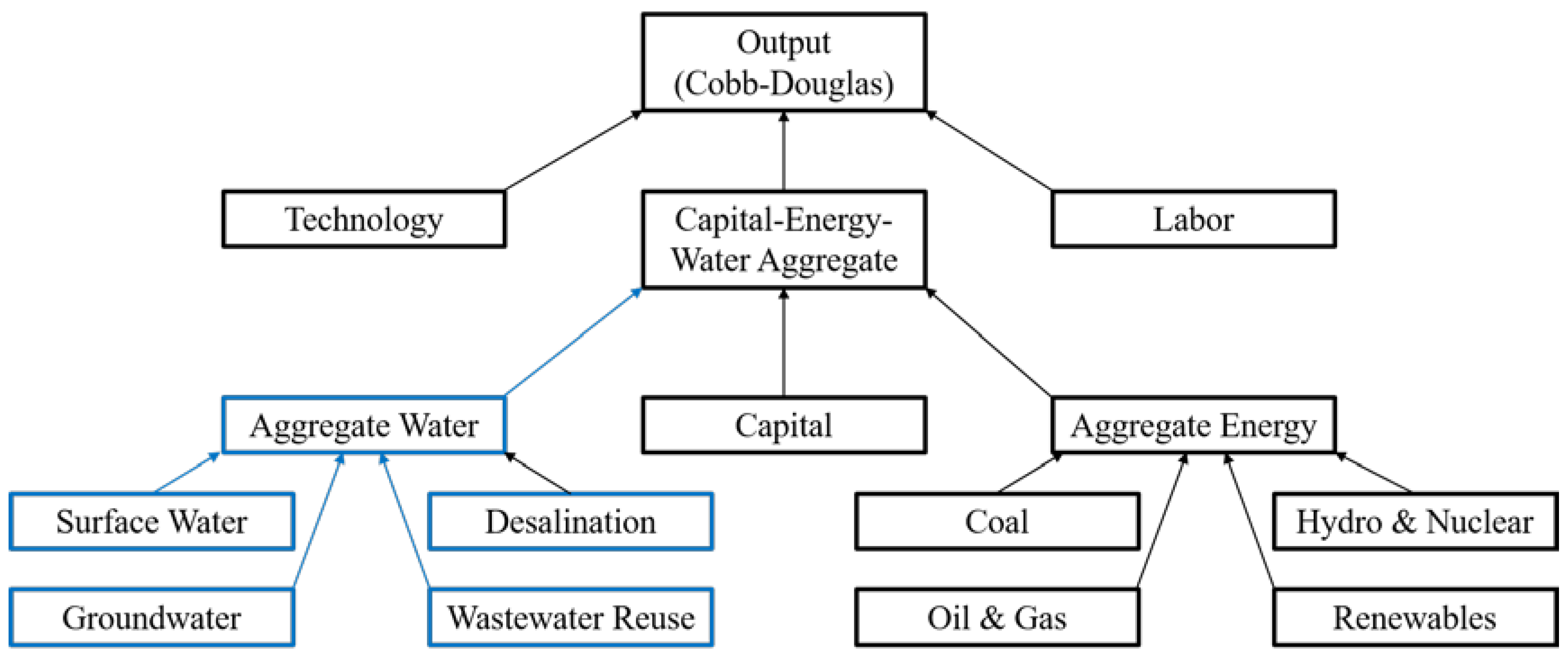
In order to include water supply development as an additional component within the energy-economy sector, key connections needed to be made with the energy-economy sector of the model. Those connections are detailed in Figure 4. Establishing these connections effectively closes several feedback loops for water supply development to fit into this sector. Water supply development is treated as an additional horizontal disaggregation of the global capital stock alongside the energy sector.

To accomplish this production structure, water production, capital, technological change and pricing structures were replicated from that of the energy economy sector. Capital stocks were created to represent water supply infrastructures for surface water, groundwater, wastewater reuse and desalination. The level of capital for each source refers to any infrastructure that relates to the global capacity of the system to provide water supply. This includes reservoirs, pumping systems, treatment systems and distribution networks. Economic output in the energy-economy sector is distributed amongst energy and water production, investment and consumption. The inclusion of water supply development adds an additional consumer of economic output (Figure 5).

3. Model Experiments

To assess future levels of water stress and the role of alternative water supplies and water quality, three experiments are used with ANEMI3 model. In the first, different formulations of water stress are compared to examine the driving factors of water stress on a global scale. The second experiment focusses on development pathways of alternative water supplies including water reclamation and reuse and desalination. Different development pathways are examined to estimate whether it is possible that sufficient supplies can be developed to alleviate global water stress. The final experiment is used to examine the potential effect of water quality on surface water supply. Here an indicator of global water quality is used to alter the production of surface water supplies, assuming that significantly lower water quality source waters are more costly to make available to the population. Each of the three experiments is discussed in detail below.

3.1. Experiment 1—Examination of Future Global Water Stress

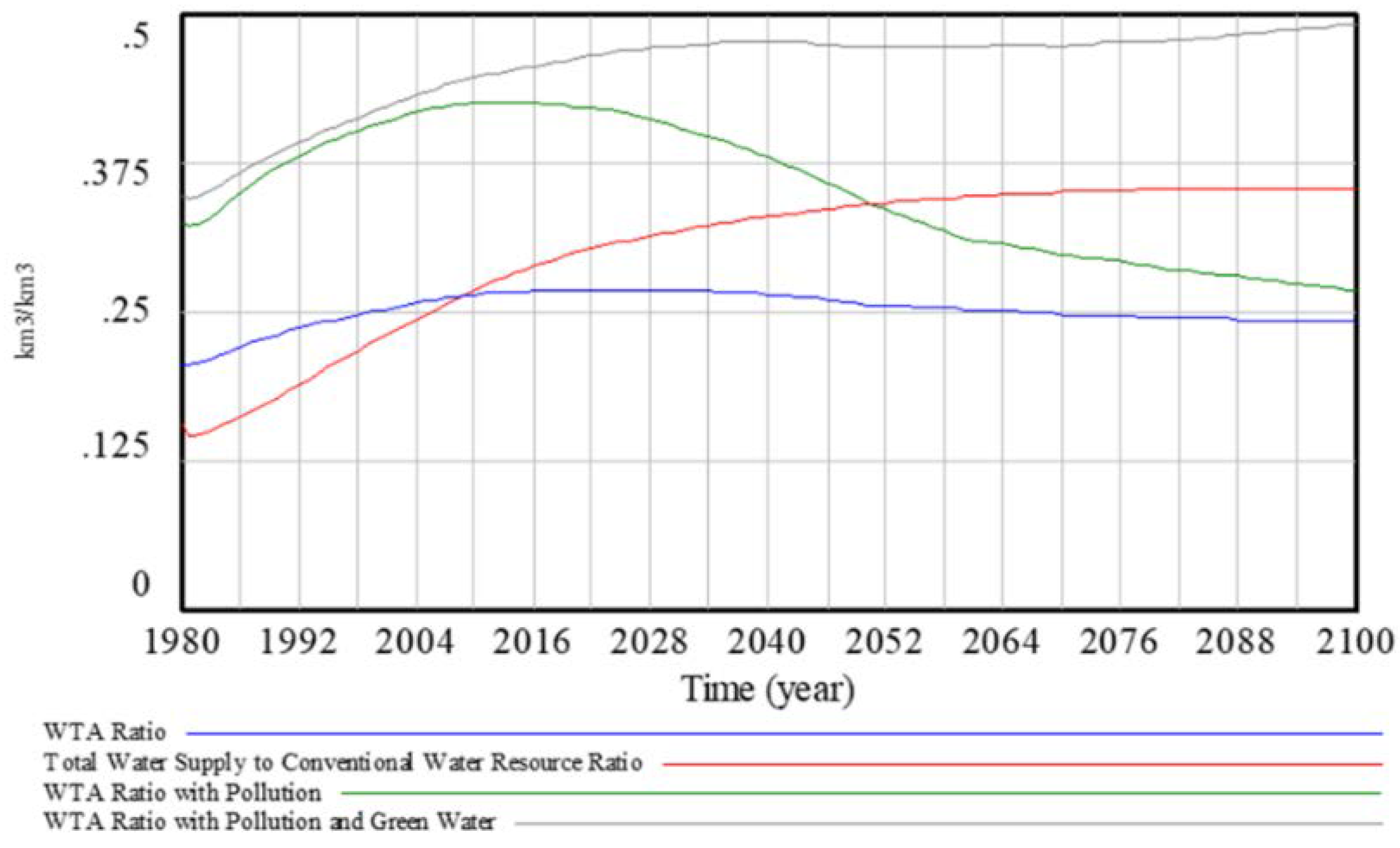
Thresholds of water stress have been defined by Reference [23]. Low, moderate, medium-high and high levels of water stress corresponds to values of less than 0.1, 0.1 to 0.2, 0.2 to 0.4 and greater than 0.4 respectively, where water stress ($WTA$) is defined as the ratio of surface water withdrawals ($SWW$) to availability ($ASW$),

$$WTA=\frac{SWW}{ASW}.$$

(9)

In the ANEMI3 model, water stress can be calculated using different formulations. Water pollution and green water dilution effects ($WT{A}_{poll}$ and $WT{A}_{poll+gw}$ can be applied to the WTA ratio in order to gain a more conservative measure of water stress [24].

$$WT{A}_{pollution}=\frac{SWW+URW\times WDF}{TotalRenewableFlow}$$

(10)

$$WT{A}_{pollution+gw}=\frac{SWW+URW\times WDF+GWR}{TotalRenewableFlow},$$

(11)

where URW = Untreated returnable water $\left[{\mathrm{km}}^3/\mathrm{y}\right]$; WPF = Water pollution factor; GWR = Green water requirement for crops and pasture $\left[{\mathrm{km}}^3/\mathrm{y}\right]$.

In this work, an additional representation is used based on the ratio of total water supply to the amount of available conventional water resources of surface water ($R_{sw}$) and groundwater ($R_{gw}$).

$$WT{A}_{watersupply}=\frac{\sum W{S}_i}{R_{sw}+R_{gw}}.$$

(12)

The total amount of water supply includes both, conventional and alternative water resources, allowing for increased alternative water resources to reduce water stress.

3.2. Experiment 2—The Role of Alternative Water Supplies

Growing populations and industrial output will increase the demand for water in the domestic, industrial and agricultural sectors, thereby increasing the pressure on freshwater resources. It is expected that these resources will become increasingly stressed over time, such that the ratio of demand to available water resources will increase. To overcome water stress, alternative supplies in addition to conventional surface water and groundwater will be needed, such as desalinated water and the wastewater reuse. The ability to analyze the distribution of water supplies through time will provide insight as to when the water resources become stressed and to what degree alternative water supplies will be needed in the future.

Alternative water supplies are represented in ANEMI3 in the same way as conventional water supplies including surface water and groundwater. However, the supply price starts at a higher value initially and is gradually reduced through improvements to the technology over time. The cost of producing alternative water supplies has decreased historically and is expected to decrease further. The rate at which technology improves in a complex system cannot be simply calculated, therefore the role of alternative water supplies in reducing future levels of water stress is examined through a Monte Carlo sensitivity analysis. The parameters used to specify technological change rates for alternative water resources is expressed using a probability distribution and the ANEMI3 model is then simulated 200 times to evaluate a range of pathways for alternative water supply development.

3.3. Experiment 3—Water Quality Effects on Surface Water Supplies

Water quality in ANEMI3 is represented by the changing concentrations of nutrient levels in surface waters. It acts as a multiplier that increases the supply price of surface water resources through hypothesized cost of increased treatment. This hypothesis is supported by the studies mentioned previously [22] but the extent of this effect is unknown and has never been looked at on a global scale. In addition to increased nutrients, wastewater inputs also render a portion of water resources unusable for the purpose of water supply, thereby contributing directly to water stress. If water quality becomes severely degraded in the future on a global scale, costs to produce water supplies could increase if technology does not progress fast enough to address potential treatment issues. Because of this, it is hypothesized that alternative water supplies may become more attractive and play a larger role in the future.

In ANEMI3, nutrient concentrations in surface waters are used as an indicator of water quality on a global scale. Wastewater and agricultural inputs are used as the main contributors to water quality degradation and changes in the levels of nutrients in the form of total nitrogen and phosphorus are used as indicators of water quality from the nutrient cycle sector of the model. The ratio of current to initial nutrient concentrations for surface water resources is used as a multiplier on the water supply price,

$$P_{w_{sw}}=P{P}_{w_{sw}}\times {\left(\frac{NCE}{NC{E}_0}\right)}^{{\gamma }_w}\left[\$/{\mathrm{km}}^3\right],$$

(13)

where $P_{w_{sw}}$ = Water supply price for surface water $\left[\$/{\mathrm{km}}^3\right]$; $P{P}_{w_{sw}}$ = Producer price for surface water $\left[\$/{\mathrm{km}}^3\right]$; NCE = Nutrient concentration effect $\left[\frac{nN·nP}{{\left({\mathrm{km}}^3/\mathrm{y}\right)}^2}\right]$; $NC{E}_0$ = Initial nutrient concentration effect $\left[\frac{nN·nP}{{\left({\mathrm{km}}^3/\mathrm{y}\right)}^2}\right]$; ${\gamma }_w$ = Influence of water quality on surface water supply price. The nutrient concentration effect takes into consideration the concentration of both total nitrogen and phosphorus,

$$NCE=\frac{N_{N_{River}}\times N_{P_{River}}}{S{F}^2}\left[\left(nN\times nP\right)/{\left({\mathrm{km}}^3/\mathrm{y}\right)}^2\right],$$

(14)

where $N_{N_{River}}$ = Nitrogen content of river stock [nN]; $N_{P_{River}}$ = Phosphorus content of river stock [nP]; SF = Streamflow $\left[{\mathrm{km}}^3/\mathrm{y}\right]$.

The effect of water quality on water supply development is examined by comparing development pathways under different levels of nutrient inputs to surface waters via wastewater. Wastewater treatment rates are set constant and compared to the baseline wastewater treatment levels.

4. Results

This section presents the results of ANEMI3 model simulations performed to address the three research questions.

4.1. Experiment 1

The projected water stress values using the formulations mentioned above are shown in Figure 6. When the effects of pollution and green water dilution are included, water stress values are much higher. Using only the WTA ratio (Equation (9)), water stress values start initially at a value of 0.21 and rise up to 0.24, which is on the low end of the medium-high water stress category. In contrast, when pollution and green water effects are considered (Equation (11)), the starting values range between 0.32 to 0.35.

As the simulation progresses, water stress with only pollution effects considered (Equation (10)) on top of the WTA reaches a peak in the year 2010 and declines afterwards. This is because in this case the pollution effects are represented only through wastewater inputs, which decrease as domestic and industrial water demands decrease in the model due to reduced water intensities with greater global economic output. When water pollution in the form of agricultural runoff or green water is included, water stress values continue to rise to a value of 0.5 by the end of the simulation. This indicates severe levels of water stress. Using the ratio of water supply to available water resource levels as an indicator of water stress results in a starting value of 0.15 which follows S-shaped growth to 0.35. This indicates a shift from low levels of water stress to the high end of the medium-high water stress category.

4.2. Experiment 2

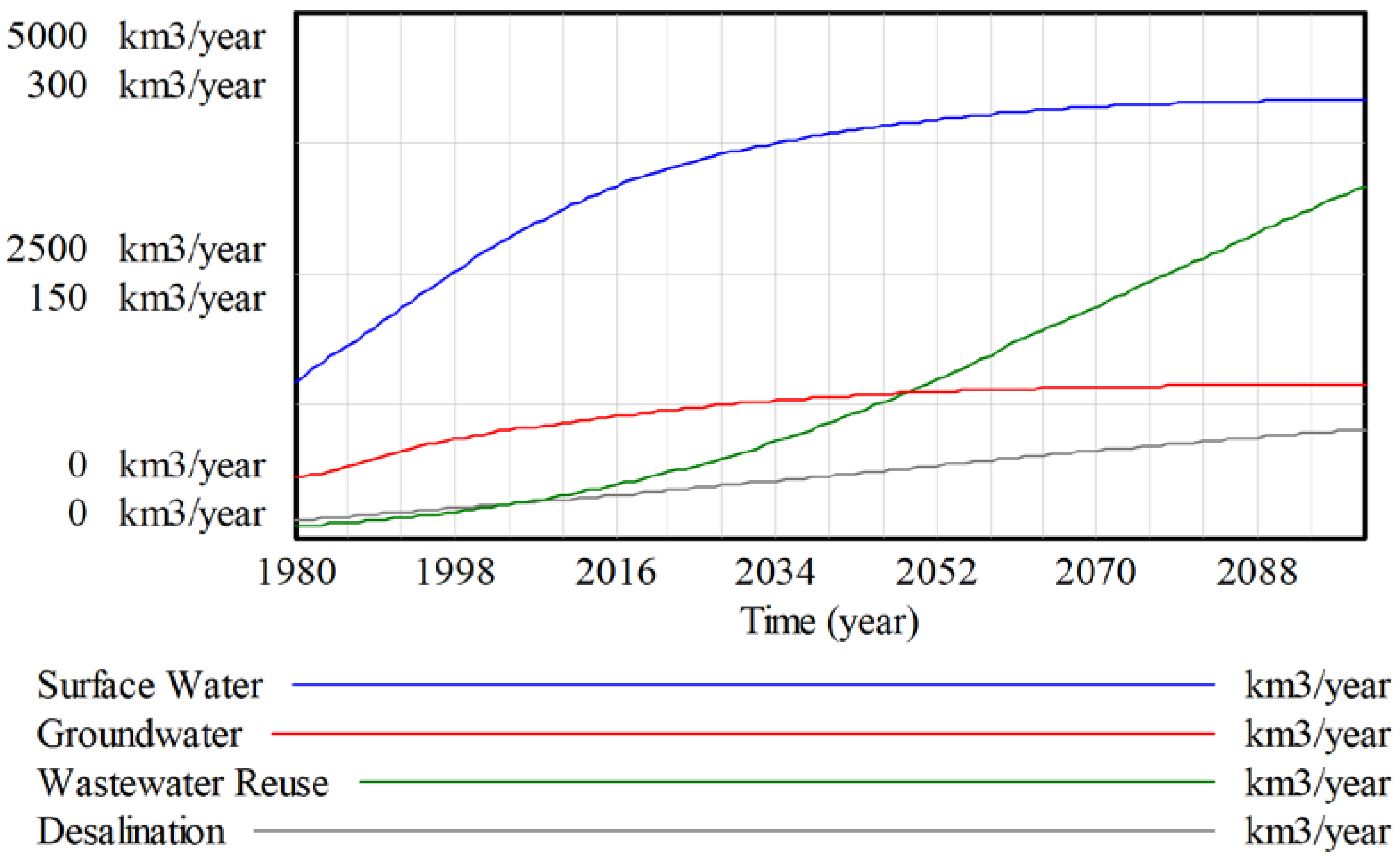
The development of water supplies for surface water, groundwater, wastewater reuse and desalination under the ANEMI3 baseline scenario are shown in Figure 7. Surface water supplies on a global scale have made up the largest fraction of water supply along with groundwater resources. They are the least costly to find and extract and there is much more capital currently invested in these supply types. However, in places where rivers or streams are not present, groundwater may be a less costly option, especially if the quality of the surface water is poor. Surface water supplies start at an initial value of 1504 km³/year and climb to a maximum of 4422 km³/year. Groundwater supplies increase at a much slower rate from 877 km³/year to 1439 km³/year. Both wastewater reuse and desalination supplies increase at a rate that is much faster than surface and groundwater, however the amounts of which are also much smaller initially, with wastewater reuse and desalination reaching 292 and 87 km³/year by the end of the century, respectively.

Surface water supplies are the dominant source of water supply globally for the ANEMI3 baseline run. This is because the supply is relatively inexpensive and abundant, compared to the other water sources on a global scale. However, this is not always the case on a regional level. There are many areas of the world where either surface or groundwater resources are currently depleted or unavailable in time and space, thus prompting the use of alternative water resources, such as desalination and wastewater reuse.

4.3. Experiment 3

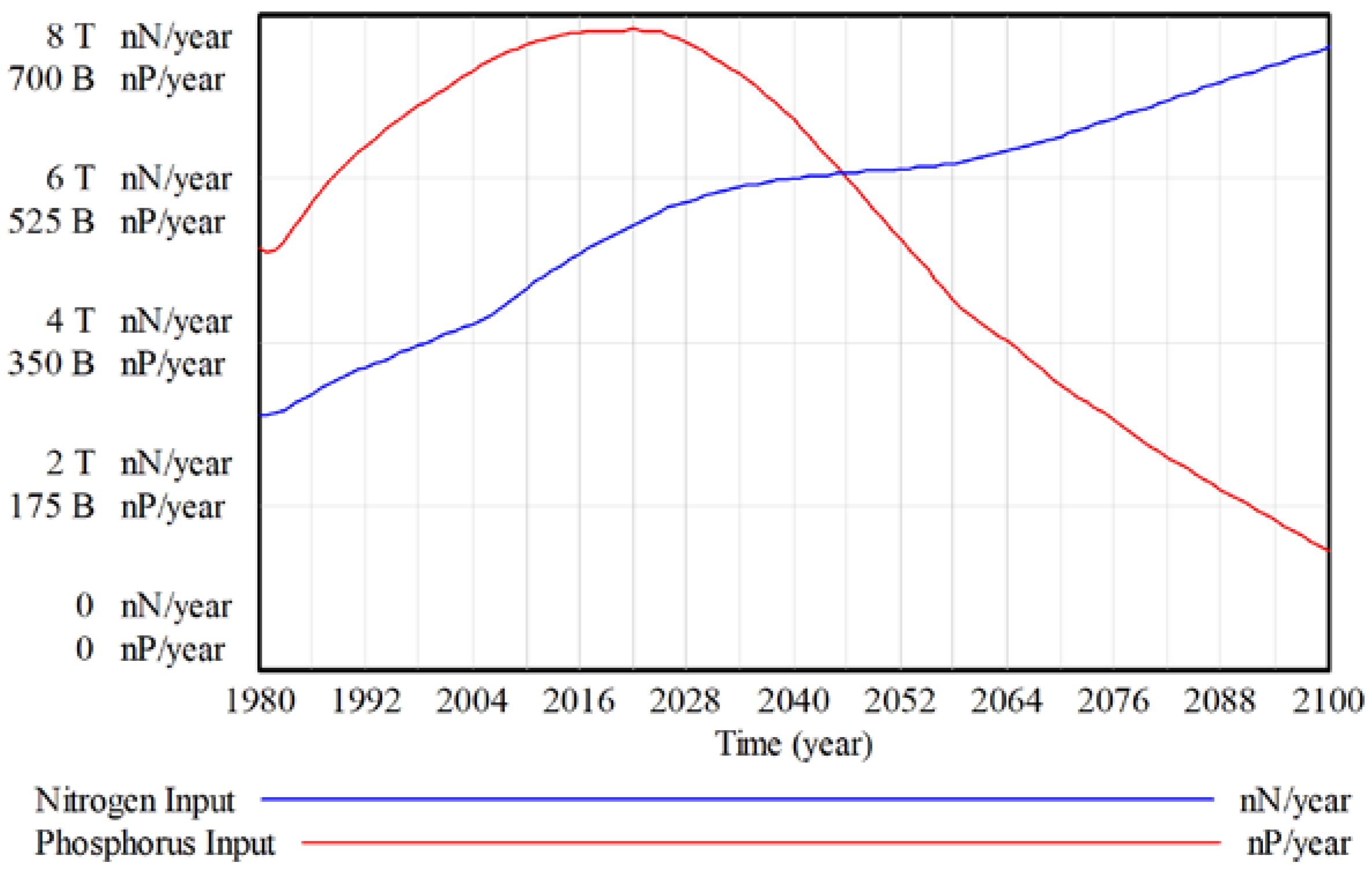
The input of nitrogen to surface waters is increasing throughout the baseline simulation starting at an initial rate of 3.1 trillion moles or 4.3 Mt per year to a rate of 7.6 trillion moles or 10.5 Mt per year (Figure 8). Input of phosphorus to surface waters on the other hand, increases from 451 billion moles or 13.5 Mt per year to a peak value of 681 billion moles or 20.4 Mt per year in the year 2025. After this point phosphorus input decreases significantly, down to 126 billion moles per year.

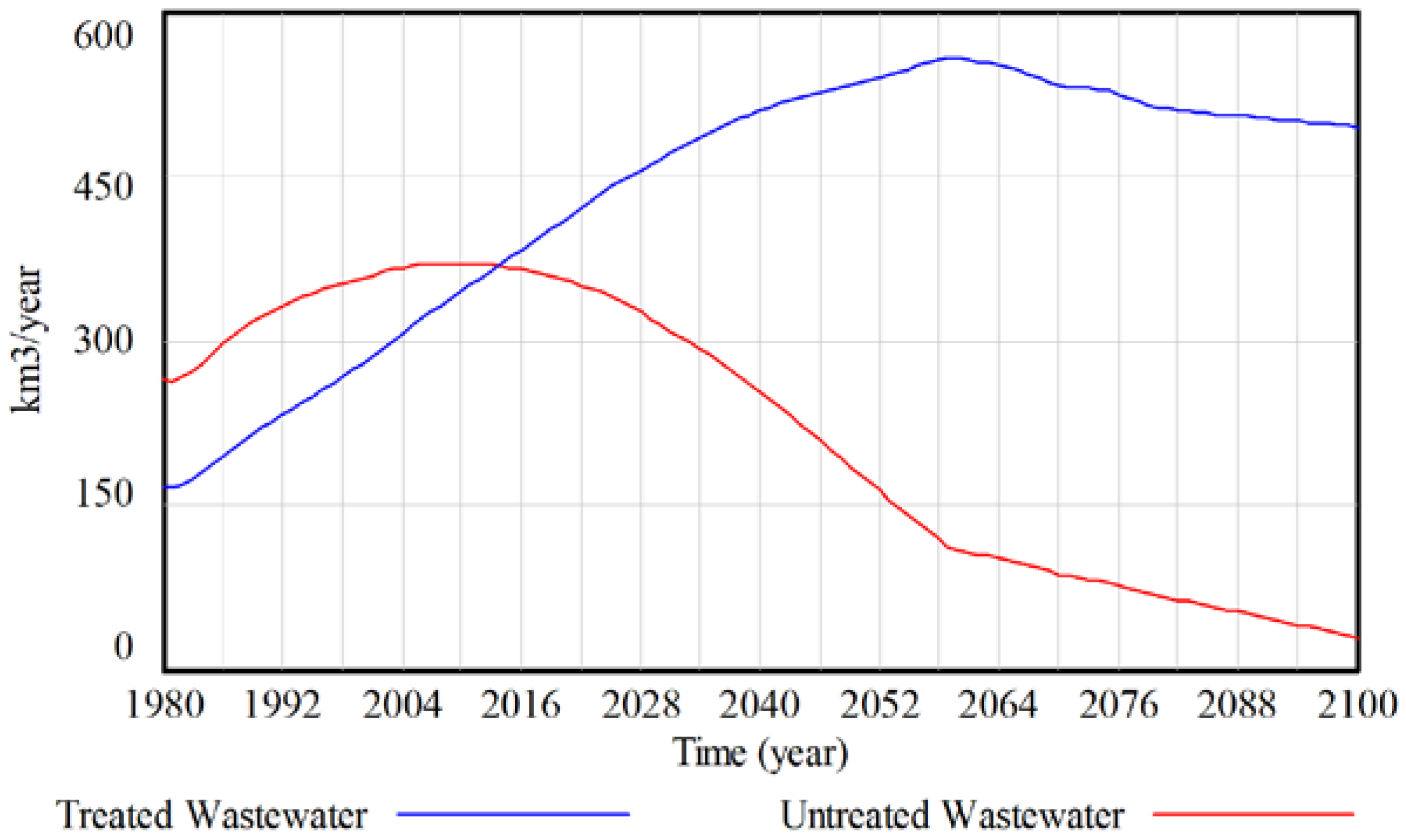
The explanation for the difference in the pattern of nitrogen and phosphorus inputs lies in their respective amounts in different sources. For nitrogen, on a global scale, agriculture is the main anthropogenic source of nutrients to surface waters, while domestic and industrial wastewaters are the main source of phosphorus. Phosphorus input decreases after the year 2025 due to increasing levels of wastewater treatment on a global scale, which reduces the input significantly. The levels of treated and untreated wastewater are shown in Figure 9. Initially, the amount of untreated wastewater is greater than treated on a global scale in 1980. Under the ANEMI3 baseline scenario, wastewater treatment increases from the initial rate of 160 km³/year and surpasses that of the untreated percentages in 2010. After this point, treatment rate increases further to approximately 550 km³/year.

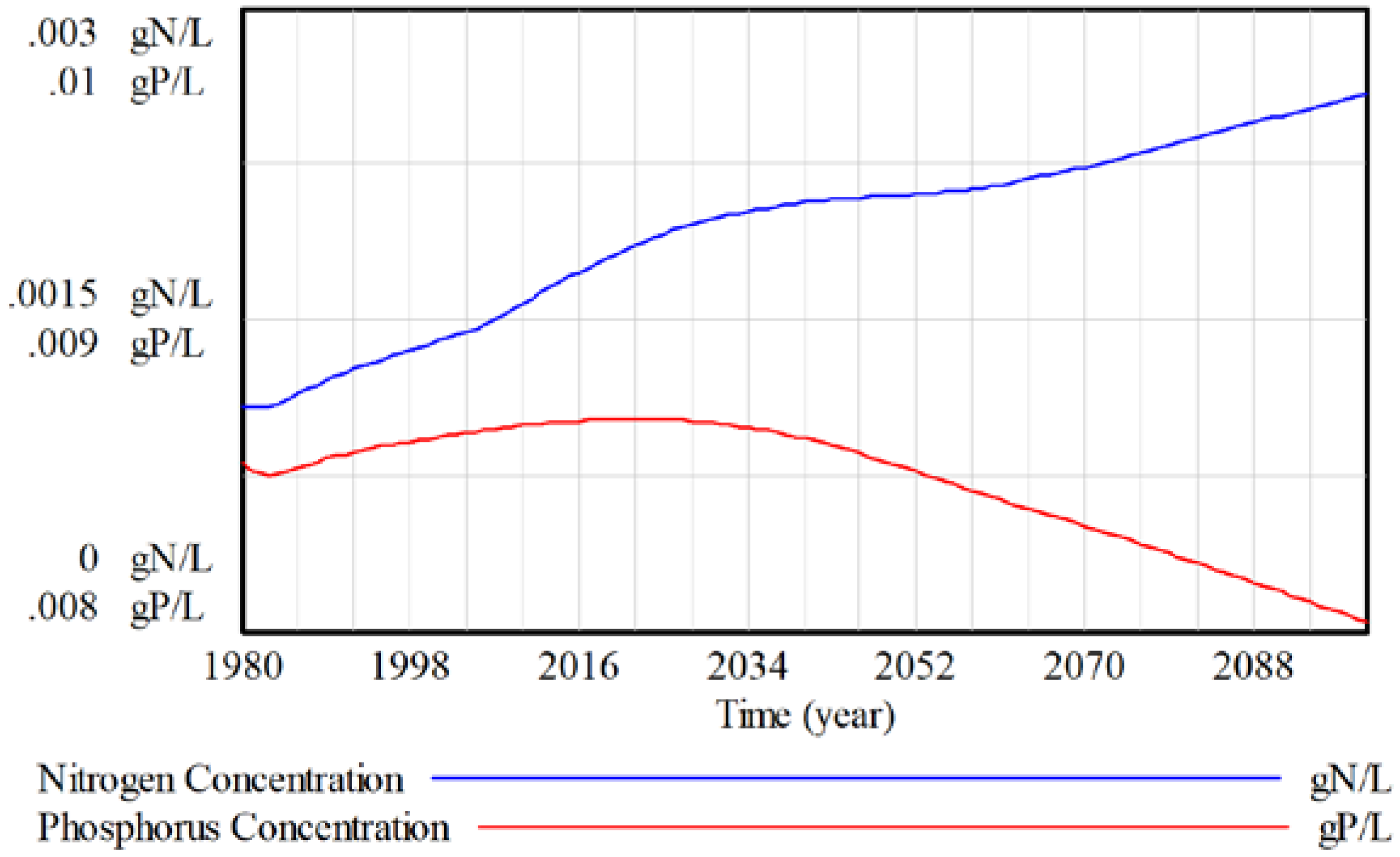
Nutrient inputs act as an additional rate that affects the surface water stock in the nutrient cycle model. Combining this with the stock of surface water in the hydrologic cycle model allows for the concentrations of nutrients in surface water on a global scale to be examined, as shown in Figure 10. The concentration considers changes in hydrologic cycle. The patterns are almost the same because the global amount of streamflow does not change very much due to climate change increase and surface water consumption having a balancing effect in the ANEMI3 baseline scenario.

Nutrient concentrations are higher when constant wastewater treatment is implemented, rather than exogenous increase in the ANEMI3 baseline scenario. Nutrient concentrations are used as an indicator for water quality in the production of surface water supplies, whereby higher concentrations act as a multiplier to the surface water production costs. The effect of constant wastewater treatment on water supply development is shown in Figure 11. Under this scenario, the establishment of surface water supplies is only slightly affected by the change in surface water quality on a global scale (Figure 11a). Under the ANEMI3 baseline parameterization scheme, water quality does not appear to play a significant role in the establishment of surface water supplies, even if wastewater treatment levels are held at constant 1980 values for the entire simulation. Both wastewater reuse and desalination supplies show major increases from 1980 to the year 2100. Wastewater reuse increases from 10 to 280 km³/year, while desalination increases from 10 to 75 m³/year, although the absolute numbers are small in comparison to conventional water supplies. With reduced wastewater treatment rates there is a major difference in the level of wastewater reuse, as there is less available wastewater resource to be used (Figure 11b). Due to scarce wastewater for reuse there is a drop from 274 km³/year to 143 km³/year by the year 2100.

5. Discussion

The paper explores the utility of adding the feedback-driven, economically based water supply development sector in ANEMI3 global change model. Capital stocks for each type of water supply grow over time with investment, which is made based on the inverse supply prices and allocated using Wood’s algorithm. Endogenous technological change is also incorporated for the desalination and wastewater reuse technologies, as well as the effects of depletion and diminishing water quality of conventional supplies.

In the ANEMI3 baseline scenario, water stress values are decreasing due to technological change and investments in water supply capital over time. The ANEMI3 baseline simulation for the development of water supplies shows that surface water resources are dominating the share of water supply during the entire simulation period from the year 1980 to 2100. This is because surface water resources are by far the least expensive option for water supply in the ANEMI3 baseline scenario. When only the global scale is considered, there is enough stable and renewable surface water resources to satisfy the demand of a growing population by the year 2100.

The potential for water quality impacts on the development of surface water supplies is assessed. Nutrient concentrations in surface water resources is calculated using the global cycles of water, nitrogen and phosphorus. The difference in sources of nitrogen and phosphorus inputs to the nutrient cycles, result in different long-term behaviors in their respective surface water concentrations.

6. Conclusions and Future Work

The ANEMI3 model structure is novel in that global water supply is able to evolve endogenously and allows for the development of conventional and alternative water supplies, while including effects of water quality on surface water resources. The development of water supply infrastructure is assessed from an economic perspective.

6.1. Main Conclusions

Under the current parameterization scheme, water quality is not shown to be a significant factor for the development of surface water supplies. When wastewater treatment rates are fixed at their initial values, surface water nutrient concentrations increase but not enough to show large impacts on surface water production.

Using increased nutrient concentrations as an indicator for water quality provides a way to represent the impact of different sources of water pollution but on a globally aggregated scale these impacts are averaged and likely understated. The reduced wastewater treatment scenario did however influence wastewater reuse. The lower quantity of treated wastewater available for reuse resulted in a greater saturation effect on the development of water supplies from wastewater reuse, thereby reducing its potential to develop as an alternative water resource.

6.2. Future Work

There are some limitations in presenting dynamics of the water supply development sector incorporated into ANEMI3 model on the global scale in the baseline ANEMI3 scenario. This is because surface water resources were enough to sustain the water demand when the available water resources consider the entire amount on Earth. This was also true for water quality, as it is averaged across the globe as well.

If the water supply development model is regionalized or adapted for use in a grid-based model, the effects of resource depletion and water quality effects on surface water supply could be explored in more detail. This is selected to be the major direction for future work. In doing this, location specific details with regards to water supply development could be considered, such as distribution costs for areas that are further away from coastlines in the case of desalination or the depth of regional aquifers for groundwater extraction costs.

References

- Steffen, W.; Sanderson, R.A.; Tyson, P.D.; Jäger, J.; Matson, P.A.; Moore III, B.; Oldfield, F.; Richardson, K.; Schellnhuber, H.J.; Turner, B.L.; et al. Global Change and the Earth System: A Planet under Pressure; Springer: Berlin/Heidelberg, Germany, 2004. [Google Scholar]
- Davies, E.G. Modelling Feedback in the Society-Biosphere-Climate System. Ph.D. Thesis, University of Western, London, ON, Canada, 2007; p. 359. Available online: http://citeseerx.ist.psu.edu/viewdoc/download?doi=10.1.1.615.378&rep=rep1&type=pdf (accessed on 19 October 2020).
- Cox, P.; Nakicenovic, N. Assessing and Simulating the Altered Functioning of the Earth System in the Anthropocene. In Earth System Analysis for Sustainability; Schellnhuber, H., Crutzen, P., Clark, W., Claussen, M., Held, H., Eds.; MIT Press: Cambridge, MA, USA, 2004; pp. 293–3124. [Google Scholar]
- Rogers, P.; Bhatia, R.; Huber, A. Water As a Social and Economic Good: How to Put the Principle into Practice; Global Water Partnership Technical Advisory Committee, Global Water Partnership/Swedish International Development Cooperation Agency: Stockholm, Sweden, 1988. [Google Scholar]
- United Nations. World Population Prospects 2019: Highlights. Dep. Econ. Soc. Aff. 2019, 1–46. Available online: https://population.un.org/wpp/Publications/Files/WPP2019_Highlights.pdf (accessed on 8 October 2020).
- Trimarchi, M.; Gleim, S. 1 Billion People May Become Climate Refugees by 2050. HowStuffWorks. 22 September 2020. Available online: https://science.howstuffworks.com/environmental/green-science/climate-refugee.htm (accessed on 8 October 2020).
- Alcamo, J.; Döll, P.; Henrichs, T.; Kaspar, F.; Lehner, B.; Rösch, T.; Siebert, S. Development and testing of the WaterGAP 2 global model of water use and availability. Hydrol. Sci. J. 2003, 48, 317–337. [Google Scholar] [CrossRef]
- Alcamo, J.; Döll, P.; Henrichs, T.; Kaspar, F.; Lehner, B.; Rösch, T.; Siebert, S. Global estimates of water withdrawals and availability under current and future “business-as-usual” conditions. Hydrol. Sci. J. 2003, 48, 339–348. [Google Scholar] [CrossRef]
- Simonović, S.P. Managing Water Resources: Methods and Tools for a Systems Approach; UNESCO, Paris and Earthscan James & James: London, UK, 2012. [Google Scholar]
- Schlosser, C.A.; Strzepek, K.; Gao, X.; Fant, C.; Blanc, É.; Paltsev, S.; Jacoby, H.; Reilly, J.; Gueneau, A. The Future of Global Water Stress: An Integrated Assessment. Earth’s Future 2014, 2, 341–361. [Google Scholar] [CrossRef]
- Aulakh, R. China wakes up to its water crisis. Toronto Star. 2014. Available online: https://www.thestar.com/news/world/2014/05/12/china_wakes_up_to_its_water_crisis.html (accessed on 18 October 2020).
- Eikebrokk, B.; Vogt, R.D.; Liltved, H. NOM increase in Northern European source waters: Discussion of possible causes and impacts on coagulation/contact filtration processes. Water Sci. Technol. Water Supply 2004, 4, 47–54. [Google Scholar] [CrossRef]
- Advisian Worley Group. The Cost of Desalination. 2019. Available online: https://www.advisian.com/en/global-perspectives/the-cost-of-desalination (accessed on 18 October 2020).
- Rotmans, J.; Dowlatabadi, H. Integrated Assessment of Climate Change: Evaluation of Methods and Strategies. In Human Choices and Climate Change: A State of the Art Report; Rayner, S., Malone, E.L., Eds.; Tol and Vellinga; Roger Jones Publishing: Harpenden, UK, 1998. [Google Scholar]
- Breach, P. Water Supply Capacity Development in the Context of Global Change; Electronic Thesis and Dissertation Repository; The University of Western: London, ON, Canada, 2020; Available online: https://ir.lib.uwo.ca/etd/6930 (accessed on 19 October 2020).
- Breach, P.; Simonovic, S.P. ANEMI 3: Tool for investigating impacts of global change. In Water Resources Research Report No. 108; Facility for Intelligent Decision Support, Department of Civil and Environmental Engineering, Eds.; The University of Western Ontario: London, ON, Canada, 2020; 134p, ISBN 978-0-7714-3146-3. Available online: https://www.eng.uwo.ca/research/iclr/fids/publications/products/108.pdf (accessed on 19 October 2020).
- Davies, E.G.R.; Simonovic, S.P. ANEMI: A new model for integrated assessment of global change. Interdiscip. Environ. Rev. 2010, 11, 127–161. [Google Scholar] [CrossRef]
- Akhtar, M.K.; Wibe, J.; Simonovic, S.P.; MacGee, J. Integrated assessment model of society-biosphere-climate-economy-energy system. Environ. Model Softw. 2013, 49, 1–21. [Google Scholar] [CrossRef]
- Breach, P.; Simonovic, S.P. ANEMI3: An updated tool for global change analysis. PLoS ONE 2020. under review. [Google Scholar]
- International Hydrological Programme. World Freshwater Resources; UNESCO: Paris, France, 2000; Volume 25, pp. 11–32. [Google Scholar]
- Wood, A.; Wollenberg, B. Power Generation, Operation and Control, 2nd ed.; Wiley: New York, NY, USA, 1996. [Google Scholar]
- Breach, P.A.; Simonovic, S.P. Wastewater Treatment Energy Recovery Potential for Adaptation to Global Change: An Integrated Assessment. Envir. Manag. 2018, 61, 624–636. [Google Scholar] [CrossRef] [PubMed]
- United Nations. Comprehensive Assessment of the Freshwater Resources of the World; Stockholm Environment Institute: Stockholm, Sweden, 1997. [Google Scholar]
- Davies, E.G.R.; Simonovic, S.P. Global water resources modeling with an integrated model of the social-economic-environmental system. Adv. Water Resour. 2011, 34, 684–700. [Google Scholar] [CrossRef]
Figure 1.
High-level feedback structure of the ANEMI3 model illustrated as a causal loop diagram (+ signs along causal relationships indicate change of connected variables in the same direction; − sign indicates change in opposite direction).
Figure 2.
Causal loop diagram of the ANEMI3 water supply development sector. The dotted arrow from water price to water supply indicates a causality that is neither positive nor negative. Different colors identify inputs coming from different model sectors. Clockwise arrow with − sign designates negative feedback loop and counter clockwise arrow with + sign designates positive feedback loop.
Figure 3.
Illustration of Wood’s algorithm.
Figure 4.
Production structure of water supply within the energy-economy-water sector of the ANEMI3.
Figure 5.
Goods allocation in the energy-water-economy sector of theANEMI3.
Figure 6.
ANEMI3 simulated levels of water stress using the withdrawal to availability ratio and alternate formulations.
Figure 7.
Development of water supplies in the ANEMI3 model. The upper scale labels are used for surface water and groundwater supply while the lower labels are for wastewater reuse and desalination.
Figure 8.
Total nitrogen and phosphorus input to surface water under the ANEMI3 baseline scenario. Left axis represents number of moles of nitrogen and phosphorus inputs to surface water per year.
Figure 9.
Treated and untreated wastewater inputs to the nutrient cycles over time.
Figure 10.
Surface water nutrient concentrations of nitrogen and phosphorus.
Figure 11.
Development of water supplies under the baseline and constant wastewater treatment scenarios for (a) conventional water supplies and (b) alternative water supplies.
Publisher’s Note: MDPI stays neutral with regard to jurisdictional claims in published maps and institutional affiliations. |
© 2020 by the authors. Licensee MDPI, Basel, Switzerland. This article is an open access article distributed under the terms and conditions of the Creative Commons Attribution (CC BY) license (http://creativecommons.org/licenses/by/4.0/).
Share and Cite
MDPI and ACS Style
Simonovic, S.P.; Breach, P.A. The Role of Water Supply Development in the Earth System. Water 2020, 12, 3349. https://doi.org/10.3390/w12123349
AMA Style
Simonovic SP, Breach PA. The Role of Water Supply Development in the Earth System. Water. 2020; 12(12):3349. https://doi.org/10.3390/w12123349
Chicago/Turabian StyleSimonovic, Slobodan P., and Patrick A. Breach. 2020. "The Role of Water Supply Development in the Earth System" Water 12, no. 12: 3349. https://doi.org/10.3390/w12123349
Note that from the first issue of 2016, this journal uses article numbers instead of page numbers. See further details here.