CliGAN: A Structurally Sensitive Convolutional Neural Network Model for Statistical Downscaling of Precipitation from Multi-Model Ensembles


Department of Geography and Environmental Studies, Wilfrid Laurier University, Waterloo, ON N2L 3C5, Canada
*
Author to whom correspondence should be addressed.
Water 2020, 12(12), 3353; https://doi.org/10.3390/w12123353
Submission received: 22 October 2020
/
Revised: 16 November 2020
/
Accepted: 25 November 2020
/
Published: 30 November 2020
(This article belongs to the Section Hydrology)
Abstract
:Despite numerous studies in statistical downscaling methodologies, there remains a lack of methods that can downscale from precipitation modeled in global climate models to regional level high resolution gridded precipitation. This paper reports a novel downscaling method using a Generative Adversarial Network (GAN), CliGAN, which can downscale large-scale annual maximum precipitation given by simulation of multiple atmosphere-ocean global climate models (AOGCM) from Coupled Model Inter-comparison Project 6 (CMIP6) to regional-level gridded annual maximum precipitation data. This framework utilizes a convolution encoder-dense decoder network to create a generative network and a similar network to create a critic network. The model is trained using an adversarial training approach. The critic uses the Wasserstein distance loss function and the generator is trained using a combination of adversarial loss Wasserstein distance, structural loss with the multi-scale structural similarity index (MSSIM), and content loss with the Nash-Sutcliff Model Efficiency (NS). The MSSIM index allowed us to gain insight into the model’s regional characteristics and shows that relying exclusively on point-based error functions, widely used in statistical downscaling, may not be enough to reliably simulate regional precipitation characteristics. Further use of structural loss functions within CNN-based downscaling methods may lead to higher quality downscaled climate model products.
1. Introduction
Despite over twenty years of studies developing statistical downscaling methodologies, there remains a lack of methods that can downscale from AOGCM precipitation to regional level high resolution gridded precipitation [1,2]. Compared to other climate variables, such as temperature or barometric pressure, precipitation is more fragmented in space, and interactions of different atmospheric scales (local, meso, synoptic) and terrestrial features are more apparent in observed precipitation patterns. It is very difficult for continuous functions used in traditional statistical downscaling methods to simulate these types of local patterns. Recent advances in machine learning (ML) methods, such as convolutional neural networks, have started to address these long-standing issues [3]. However, widely used loss functions, such as mean absolute error (MAE) and Nash-Sutcliffe efficiency (NS), consider overall simulation performance but ignore the spatial structure of precipitation; a key property if replicating observed local patterns is an objective [4]. Narrowly defined loss functions inhibit the potential of machine learning methods in downscaling, leading to the poor performance of models at regional scales.
Synoptic scale climate variables are commonly simulated by coupled atmosphere–ocean global climate models (AOGCMs), which provide a numerical framework of climate systems based on the physio-chemical and biological characteristics of their components and feedback interactions [5]. Coupled AOGCMs are computational frameworks that can simulate an estimate of the spatio-temporal behavior of different climatic variables under the effects of variable concentrations of greenhouse gases (GHG) in the atmosphere [6]. Physically-based representations of the physics and chemistry of the atmosphere and oceans make these models one of the most reliable tools for deriving future projections of meteorological variables (temperature, humidity, precipitation, wind speed, solar radiation, pressure, etc.). AOGCMs can simulate estimates of atmospheric variables which can be treated as possible representations of future climate [7].
AOGCMs degrade at higher spatial and temporal scales [8]. AOGCMs typically run with a spatial resolution of 250 km to 600 km, the scale at which AOGCMs can capture synoptic-scale circulation patterns and correctly simulate smoothly varying fields, such as surface pressure. As the physical assumptions underlying the various parameterizations in AOGCMs target this scale of “variable resolving resolution”, we can place a high level of confidence on the estimates over those scales. However, as we move from the synoptic scale into finer hydrologically relevant scales and analyze highly spatially heterogeneous fields such as precipitation, AOGCM skill quickly deteriorates [9] The coarse resolution of AOGCMs tends to distort the representation of regional variations of precipitation which, in turn, can alter the formation of site-specific precipitation conditions by affecting the sub-grid-scale processes. Various assumptions in the parametrization of different processes, different resolutions of land covers and topography, and their representations [10], and varying solution methods of different AOGCMs (FEM, FVM, etc.) can affect their estimation of climatic variables. As such, ensemble methods attempt to capture a suite of AOGCMs by collating outputs from multiple models, which in turn aims to reduce sensitivity to individual model biases through a quantitative framework [11]. Failure of models in predicting highly variable processes driving, for example, daily precipitation, limits their utility in several applied and management settings [12,13].
To study a climatic variable at hydrological or regional scales, we need to reduce the scale of the outputs from climate models. The method used to reduce the scale of the AOGCM’s output is broadly referred to as “downscaling”. As per the design and methodology, downscaling procedures are broadly classified into two different types, namely dynamical downscaling and statistical downscaling. In dynamic downscaling the most common approach is to use a regional circulation model (RCM) or limited area model (LAM) that are designed to operate at a higher spatial resolution to simulate climatic variables of interest using AOGCM simulated fields as initial and boundary conditions [13]. But experimental design complexity and computational effort make this approach infeasible when multiple ensembles of AOGCMs are required in the study [14,15]
Useful features of statistical downscaling are its simple architecture and less computational burden compared to the dynamic downscaling [15]. Statistical downscaling can produce synthetic variables of any prescribed length which makes it very popular in studies of climate change impacts [16]. The statistical downscaling draws the empirical relationships between the regional scale predictants (variables of interest) and predictors (AOGCMs) and constructs regional-scale atmospheric variable structure from large-scale simulated patterns. [17] explained the underlying assumptions which created the basis of subsequent statistical downscaling methods. The robustness of statistical downscaling to study climate change impact of any region can partly be attributed to its methodology to incorporate historical observations that carry the location-specific climatic signature. The comparison of statistical and dynamic downscaling methods over Northern Canada by [18] showed that the biases in precipitation estimates were lower in statistical downscaling and the distributions of maximum and minimum temperatures were well estimated.
Statistical downscaling methods are broadly classified into three different categories based on their design of processing the predictors and predictants [19,20]: (i) weather generators, (ii) weather typing, and (iii) transfer functions. Stochastic weather generators are essentially complex random number generators, which can be used to produce a synthetic series of data [21]. This feature enables researchers to address natural variability when studying the impact of climate change. Brissette et al., 2007 classified weather generators into three types, (i) parametric [22,23,24,25,26], (ii) semi-parametric or empirical [27,28] and (iii) non-parametric [29,30,31]. A detailed discussion of these methods is beyond the scope of this paper but it should be noted that one of the key advantages of weather generators is their ability to produce synthetic time series of climate data of the desired length based on the statistical characteristics of the observed weather. Weather typing approaches [32] involve the clustering of regional-scale meteorological variables and linking them with different classes of atmospheric circulation. Within this framework, future regional climate scenarios can be generated in two different ways: (i) by re-sampling from the observed variable distribution given the distribution of circulation pattern produced by a GCM, or (ii) by the Monte Carlo (MC) technique producing a synthetic sequence of weather patterns and based on that sequence re-sampling from the archived data. The relative frequency of different types of weather patterns are then weighed to estimate the moments or the frequencies of the distribution for the regional-scale climate.
Perhaps the most popular approach within statistical downscaling methods is transfer functions, which is a regression-based framework [33,34,35,36]. The method consists of developing a direct functional relationship between global large-scale variables (predictors) and local regional-scale variables (predictants) through the statistical fitting. One method can differ from the other on the choice of mathematical functions, predictor variables, and procedure of deriving relationship. There have been several studies focused on the application of neural networks [37,38], regression-based methods [38], support vector machine [36], and analog methods [39] in statistical downscaling. Artificial neural networks (ANN), due to their robust nature in capturing the nonlinear relationship between predictors and predictants, have gained wide recognition in the climate modeling community [33,38,40,41].
More recently, the use of machine learning and data science methods has increased in various fields owing to their superior performance and robust methods/software implementations. Specifically, convolution neural network (CNN) modeling has gained wide popularity because of lower computational requirements compared to the dense networks through the extraction of spatial information through kernel filters [42]. There is a wide range of applications of CNNs including image recognition [43], image segmentation [44], and satellite image change detection [45]. Image super-resolution [46] is another method where CNNs have been applied to increase the resolution of an image, an application analogous to the climate model downscaling context.
Among the climatological variables that are in general downscaled in practice, precipitation, perhaps, is most susceptible to various uncertainties [47]. The non-Gaussian nature of extreme precipitation owing to its localized nature creates problems for classical statistical estimators [48,49]. Some recent studies have utilized more advanced statistical techniques and Bayesian methods in particular to downscale extreme precipitation over data sparse regions [50,51]. An example of direct application of machine learning techniques in statistical downscaling of precipitation is [52] who used a generalized stacked super-resolution CNN to downscale daily precipitation over the US. Despite several limitations in their experiments, the result shows the efficiency and robustness of the approach over other methods in predicting extremes. [53] also recently introduced a novel residual dense block (RDB) into the Laplacian pyramid super-resolution network (LapSRN) to generate high-resolution precipitation forecast. [54] used super-resolution techniques to simulate high-resolution urban micrometeorology, while [55] proposed several CNN-based architectures to forecast high-resolution precipitation. Underlying all of these models is the treatment of two-dimensional fields such as climate model outputs and gridded observations as analogous to non-geographic images which makes CNNs an ideal candidate as transfer functions in statistical downscaling.
Recent advancements in machine learning strategies have developed several algorithms for image super-resolution, for example, attention-based training [56,57]. One such recent advance, generative adversarial training (GAN), was proposed by [58] where two networks compete in a zero-sum game that has been used widely to train deep neural networks in recent years. This method provides a superior training of network and can produce outputs that look superficially close to reality to human observers and address the gradient problem in an intuitive way. Ref. [59] used adversarial learning to downscale wind and solar output from several AOGCM climate scenarios to regional level high-resolution. Cheng et al., 2020 also used adversarial learning to downscale precipitation. Their result shows the promising performance of the generative adversarial network in downscaling climate data.
In this paper, we develop a novel downscaling method using GAN, which can downscale an ensemble of large-scale annual maximum precipitation given by several AOGCMs to the regional-level gridded annual maximum precipitation. The objectives of our study are the following;
- Develop a methodology to downscale large-scale precipitation, given by several AOGCMs, to regional-scale precipitation by statistical downscaling using convolution neural network and generative adversarial training.
- Propose a novel loss function which is a combination of content loss, structural loss, and adversarial loss, which improves the prediction of global and regional qualities of the downscaled precipitation.
2. Methods
2.1. Study Area and Datasets
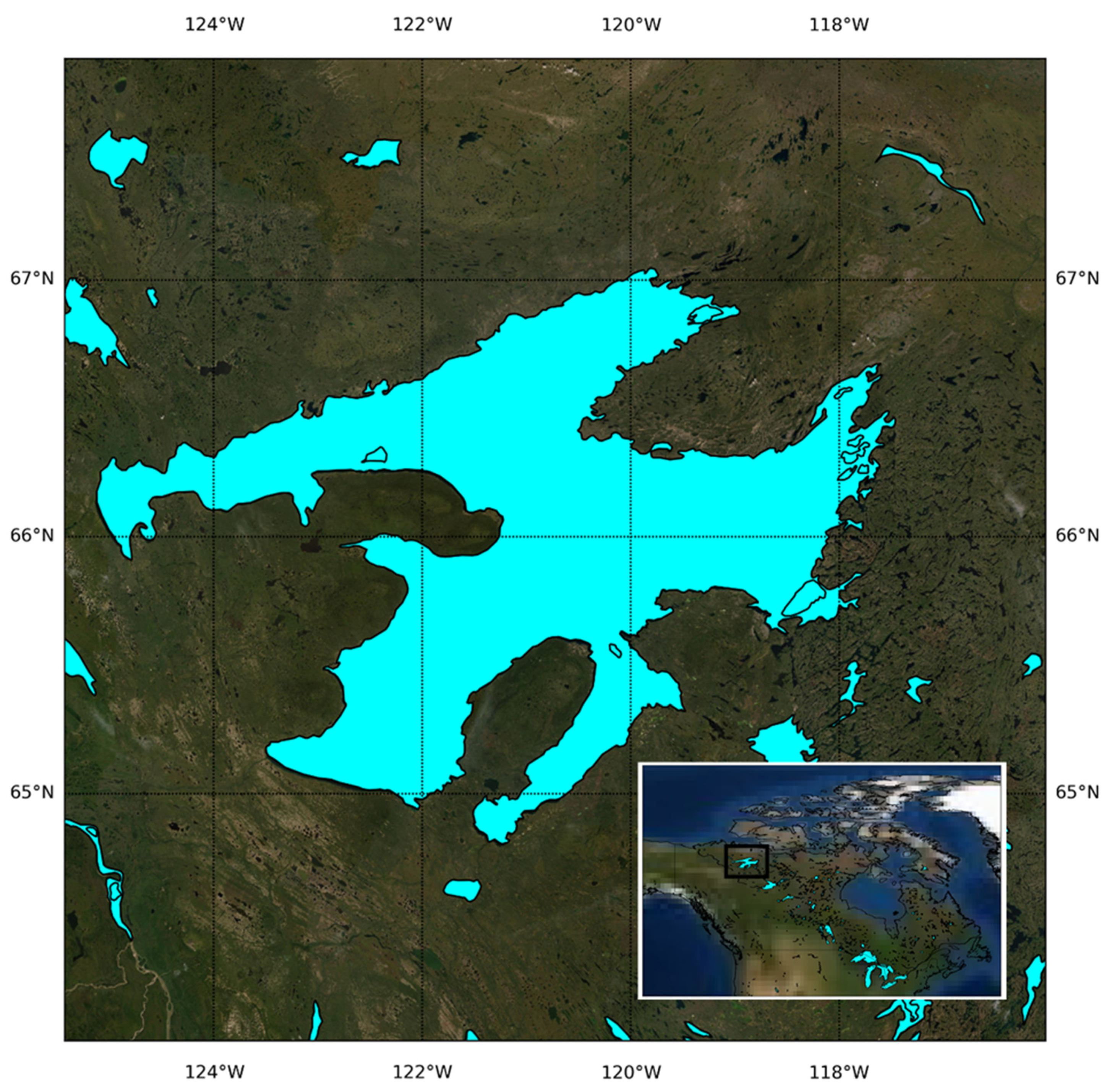
The Tsá Túé Biosphere Reserve is situated around Great Bear Lake in Northwest Territories, Canada. Great Bear Lake is the last large pristine arctic lake, covering an area over 31,000 km2. The rate of environmental change in northern Canada has been widely documented, including landform transformation [60], shrub expansion in the tundra [61], permafrost thaw and related hydrological impacts [62], wildlife declines [63], and changes affecting local communities and culture [64]. Furthermore, scarce weather data due to sparse observational stations make the estimation of the change through in-situ observation more difficult. It is evident the local communities in Canada’s north need to adapt and prepare for the anticipated impacts of climate change with help of the climatic data at hydrologically-relevant scales. This sets up a critical need for better climate impact prediction and estimation at regional scales. Figure 1 shows Great Bear Lake and its adjacent regions within Tsá Túé Biosphere Reserve, which is used as a downscaling region of interest in this study.
We developed this downscaling methodology using annual maximum daily precipitation as our target variable. Annual maximum daily precipitation data during 1950–2010 were extracted from the NRCANMET daily gridded precipitation dataset [65]. While gridded data derived from a sparse observation network in northern Canada are not ideal validation data, these are the best available for the region and should replicate regional patterns. [38], and [66], in their studies discussed the properties of any predictor in statistical downscaling. They should be (1) reliably simulated by GCMs, (2) readily available from the archives of GCM outputs, and (3) strongly correlated with the surface variables of interest (rainfall in the present case). The simulated rainfall by GCMs contains the dynamical information of the atmosphere as well as the information of the effects of climate change on rainfall, through different physical parameterizations. We therefore utilized the AOGCM simulated precipitation as a predictor of the observed (i.e., gridded) precipitation. Our statistical framework will not only create the fine resolution precipitation but will correct the biases of the AOGCM simulated precipitations as well.
Nine AOGCMs from the CMIP6 archive were selected for this study (Table 1). Different AOGCMs have different grid resolutions and many are represented in Gaussian grids, which makes it hard to treat them within a common mathematical framework. To overcome this difficulty, we interpolated precipitation from different AOGCMs onto 10 km resolution grids using bi-linear interpolation method.
2.2. Downscaling Method
We train a generating network which can transform coarse resolution AOGCM extreme precipitation (PGCM) to regional scale fine resolution extreme precipitation (Pobs). The technical difficulties of the problem involve increment of the resolution, bias correction, and regional scale precipitation feature corrections. The number of training years y=1,…, n then the θG is obtained through solving the minimization of the downscaling total loss function :
We designed the downscaling total loss as a weighted combination of several components. We discuss these components in detail later.
2.2.1. Adversarial Training
We used Wasserstein GAN (WGAN) [67] as a discriminative network. It uses the Earth-Mover (also called Wasserstein-1) distance W(q, p), which is informally defined as the minimum cost of transporting mass to transform the distribution q into the distribution p (where the cost is mass times transport distance).
Formally, the game between the generator and the discriminator is a minimax objective. The WGAN value function is constructed using the Kantorovich–Rubinstein [68] duality to obtain:
where is the set of 1-Lipschitz functions. To enforce the Lipschitz constraint on the WGAN, [67] propose to clip the weights of the WGAN to lie within a compact space [−c, c]. The set of functions satisfying this constraint is a subset of the k-Lipschitz functions for some k which depends on c and the WGAN architecture.
2.2.2. Downscaling Total Loss
The total loss is designed as a linear combination of 3-loss components: adversarial loss, content loss, and structural loss.
Adversarial loss:
The adversarial loss is given by the approximate earth moving distance between the observation and generator output. It is given by:
Content loss:
The Nash–Sutcliffe model efficiency coefficient (NSE) is a widely popular loss estimate which assesses the predictive ability of any hydrology model. We have taken (1-NSE) as content loss:
This loss can take range 0 to . 0 loss means a perfect match with the observation. The loss value 1 means that the model is as accurate as of the average of the observed values. The loss greater than 1 signifies that the observed mean is a better predictor than the model.
Structural Loss:
The overall low error may not conserve the regional relevant details common to high-resolution precipitation. To address this problem and conserve the regional details we introduced a structural loss function. Multi-scale structural similarity index (MSSIM) [69] compares the luminance, contrast, and structure of two 2D fields. We compared this metric on multiple scales to preserve the regional scale structure of the precipitation at those scales. We defined our loss based on structural dissimilarity (DSSIM) which is defined by (1 − MSSIM)/2;
where the highest scale or the window size is given by M. , , and are weights of luminance, contrast, and structure components respectively at scale i. We used α = β = γ = 1. For any given scale the luminance comparison is given by:
The contrast comparison is given by:
and the structure comparison is given by:
where and are the mean of observation and generated values, respectively; and are the standard deviation of observation and generated values, respectively; and is the co-variance between observation and generated values. , , and are small constants to stabilize the divisions with weak denominator. We used , , where , , and is the dynamic range of the input which we have taken as 100.
2.2.3. Networks
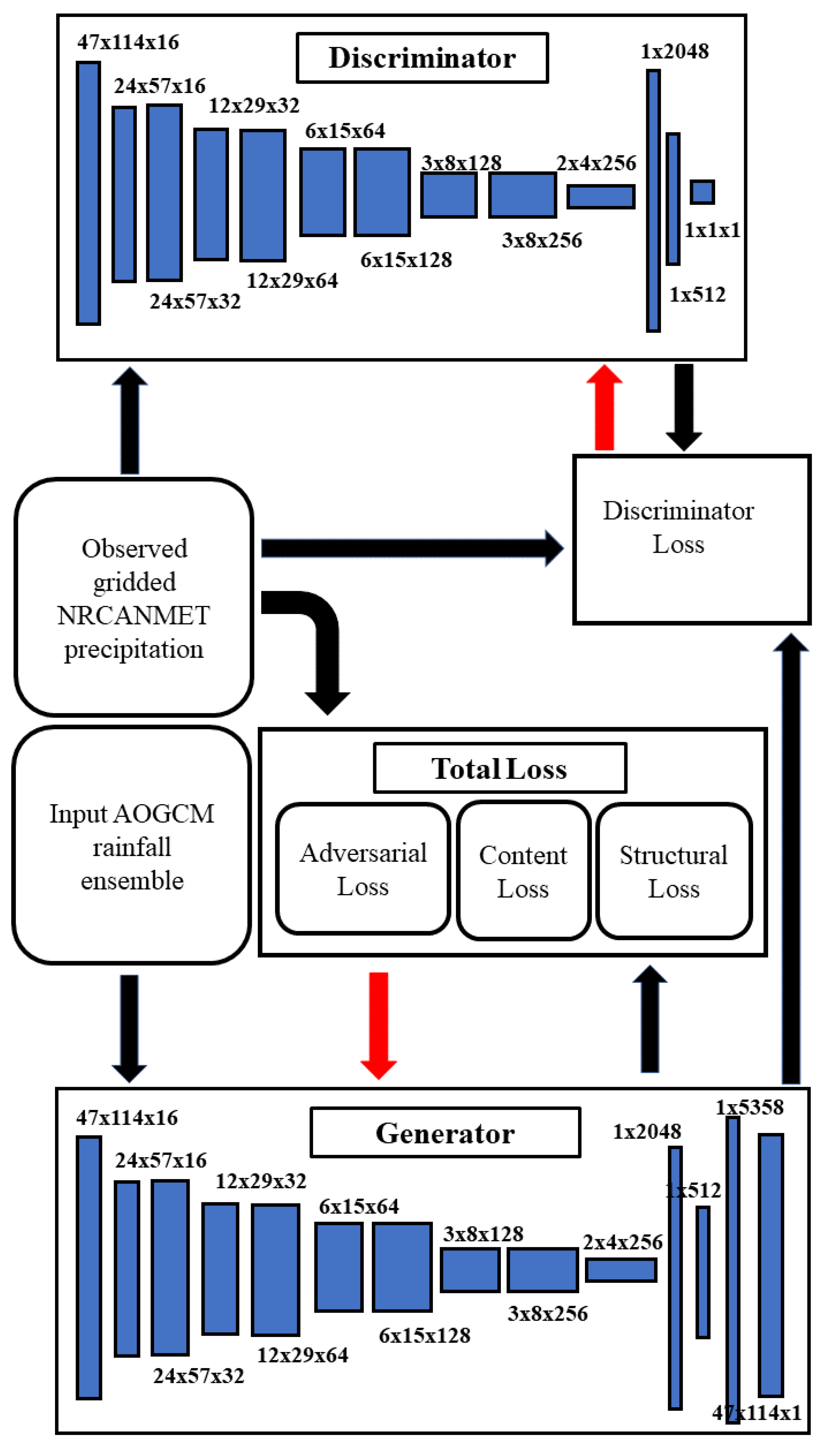
The generative network is built in the style of convolution encoder and dense decoder. We used LeakyReLU with momentum 0.2 to activate the hidden layers and used strided convolution for downsampling. ReLU has been used in the last layer of the Generator. We used L2-norm regularization with weights 1−5 on model weights and biases to prevent over-fitting.
Like the generative network, the discriminative network has a convolution encoder with a strided convolution downsampler. We used the LeakyReLU with momentum 0.2 as activation in the hidden layer and ReLU activation is used in the output layer. Batch normalization with momentum 0.8 is used after every convolutional layer to stabilize the training. The discriminative network computes the approximate earth moving distance (Wasserstein distance) between the observed and predicted precipitation. Following the recommendation of WGAN, we created compact support for layer weights by clipping them between [−1, 1]. The schematic for the networks and training procedure is shown in Figure 2. The CliGAN model was implemented in python and is available via request from the authors.
2.2.4. Training Details
Model training was performed on the NVIDIA Quadro 4000 GPU (Santa Clara, CA, USA). The l2-norm regularization was used on both weight and bias of the generator to prevent over-fitting. Furthermore, we employed a random sub-sampling strategy to train the network to capture the stochasticity of the entire population. The entire dataset is temporally split into random training and testing set for each training epoch. The network is trained using the training set and the performance is tested on the testing set. We used 66%/33% training/testing data divide, which resulted in 41 temporal points for training and 20 temporal points for testing. We avoided any kind of rescaling of the input or output data and allowed the model to learn and evolve the climate signal present in the different model datasets and observations. The generator was optimized using Adam first-order gradient-based optimization [70] based on the Linf norm (Adamax) [71] with initial learning rate m = 0.02 and decay 0.5. We wanted the discriminator to compute the gradient-based on an adaptive window near the present iteration and did not want to use all the previous generator results of the gradient information. Therefore, we used a moving window update of the gradient in Adam (Adadelta) [72] to train the discriminator Wasserstein distance computer. The initial 500 iterations were discarded as burn-in and subsequently the model was trained for 10,000 iterations until convergence. These settings were found to be more than adequate for simulating realistic high-resolution precipitation patterns.
To compare the performance of generative adversarial training we trained two more models. In the 1st alternative network traditional mean absolute error has been used to train the generator instead of a combination of loss applied in the CliGAN. We also trained a second alternative model inspired by [2]. In this model, the first 10 principal components with the largest eigenvalues from each of the nine climate models are mapped to the 20 principal components (~99% variance explained) of the observation using a single layer neural network. The overfitting of the network is prevented using a 0.5 neuron dropout rate between the layers. More details on the climate model eigen spectra, observation eigen spectra, and training performance of the network are given in the reference section of the paper.
3. Results and Discussion
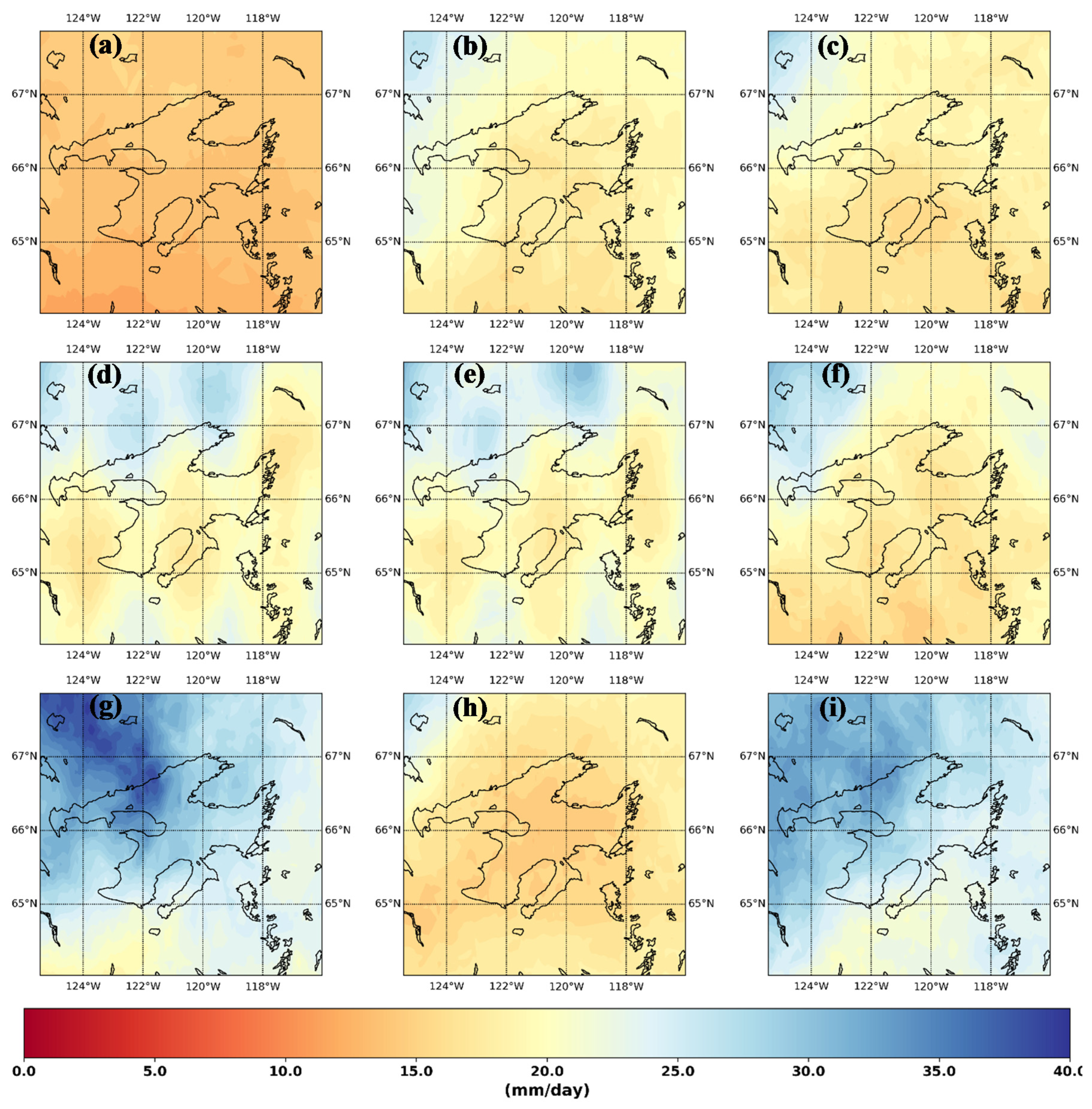
The median annual maximum rainfall generated by the various AOGCMs examined in this study varied considerably (Figure 3), indicating significant inter-model uncertainty and the need for an ensemble approach [73]. One of the major challenges in downscaling these precipitation variables to any region is to correct these biases (or differences) according to the observed pattern [74]. An ideal downscaling method not only generates a higher resolution regional level realization of the climatic variable but should also reproduce both patterns and magnitudes. The models examined here show the need for downscaling methods that can produce a spatial and temporally coherent observed climatic distribution.
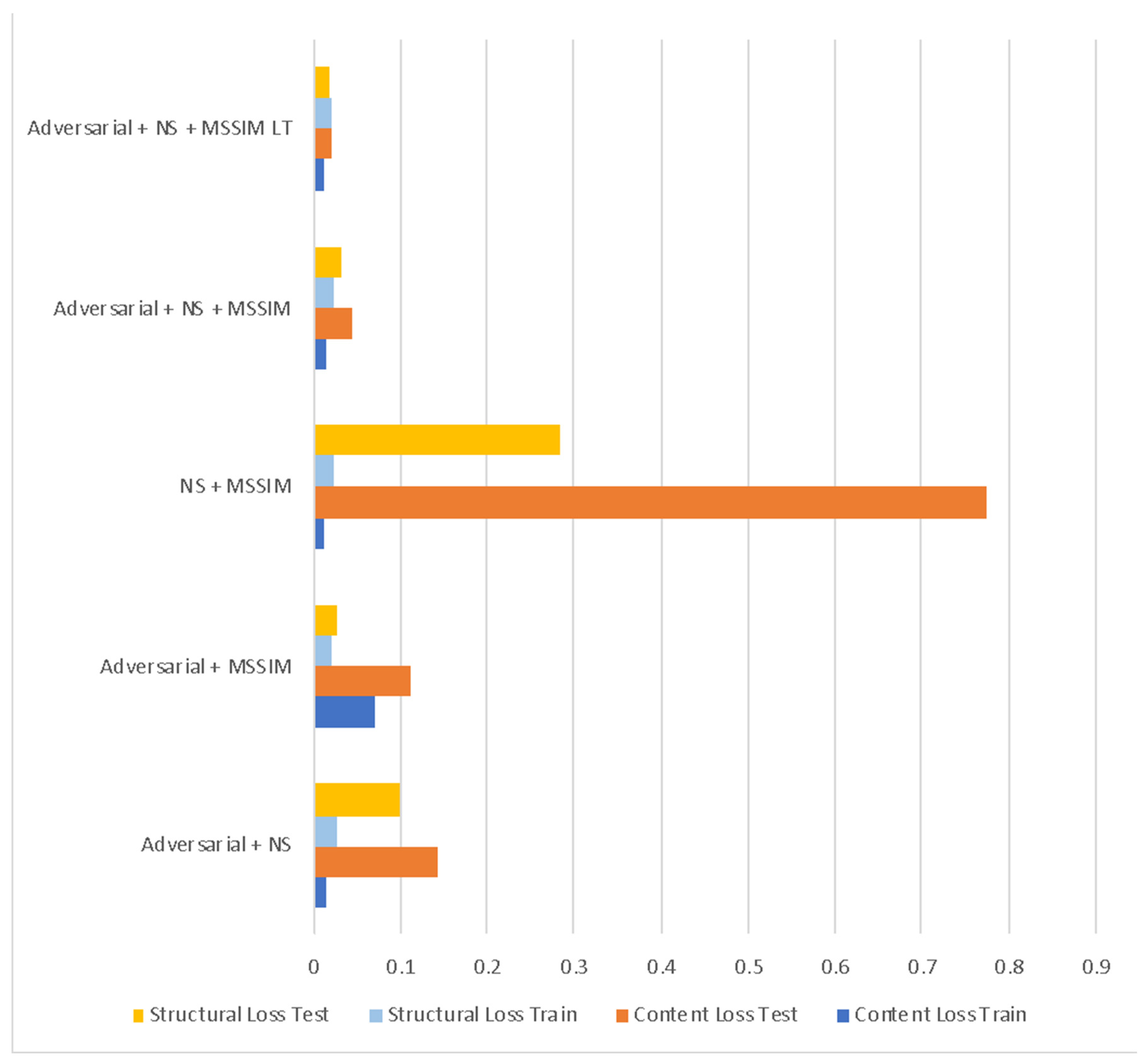
A key contribution in the CliGAN modeling framework is the development of a novel loss training method incorporating the spatial structure of rainfall. To validate our use of the total loss functions, we experimented with different combinations of loss functions (Table 2). Each model is trained with a different permutation of loss functions for 10,000 iterations; and the median training and testing loss of the last 50 iterations is reported in the table. The combination of all three— adversarial loss, NS loss, and MSSIM loss—has content errors of 0.015 and 0.043, and structural error of 0.024 and 0.033 for training and testing, respectively. It can also be noticed the adversarial loss plays a vital role in stabilizing the performance of the network (Figure 4). Even though the training results are similar magnitude for all the experiments, the inclusion of the adversarial loss function in the combination of loss functions, have produced testing results order of magnitude improved results for the testing set. The total loss combination is found to be producing a balanced error for both content and structural error and performed stable for both training and testing. Thus, we go forward with this total loss combination. To validate the model, we trained the total loss combination for 20,000 iterations the content losses are found to be 0.011 and 0.020, and structural losses are found to be 0.021 and 0.017 for training and testing, respectively. This justifies our choice of using this loss function.
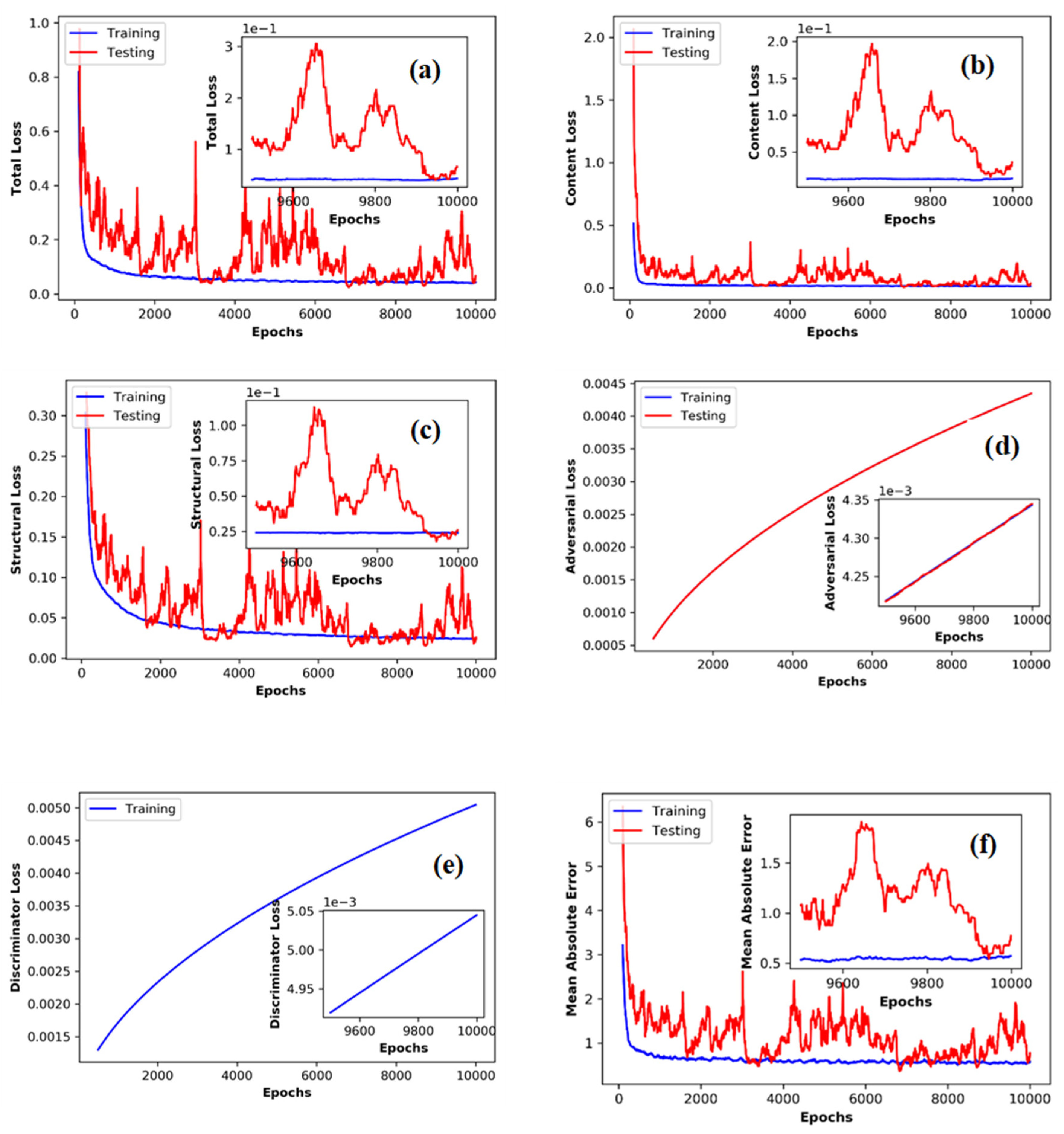
Figure 5 shows the trace of different training and testing losses for all the loss function combination error function for 10,000 iterations. For total, content, structural loss first 100 iteration results are discarded as part of generator warm-up and for adversarial loss and discriminator loss first 500 iterations are discarded as part of discriminator spin up. Figure 5a shows the trace of the total loss. Considering this is a combination of three types of errors—adversarial error, content error, and structural error—it does not have any meaningful unit. Figure 5b shows the trace of content loss and Figure 5c shows the trace of the structural loss. Notice the stable training trace and fluctuating testing trace. However, overall, the testing error is showing a decreasing trend for both content and structural loss. The adversarial loss keeps on increasing (Figure 5d) for both training and testing. This signifies the ability of the discriminator to distinguish generator output and observation. The training loss of the discriminator (Figure 5e) shows the increasing trace. However, it is marginally greater in magnitude than adversarial loss. This means the generator is doing a good job of emulating the observed patterns. Mean absolute error trace (Figure 5f) shows a pattern like content loss.
For the final simulation, we trained the model with all the available input data. This also enabled us to compare the model against other models effectively. For the total loss of the model, error continued to decrease even after 10,000 iterations (Figure 6a). The content loss stabilized around a value 1−3 after 10,000 iterations (Figure 6b), while the structural loss stabilized around a value of 2.4−2 (Figure 6c). The adversarial loss in Figure 6d keeps on increasing after 10,000 iterations indicating the discriminator is resolving the differences between the observed and predicted precipitation patterns. The discriminator error also keeps on increasing (Figure 6e), signifying the good performance of the generator. However, the loss of the discriminator is still lower than the adversarial error. As an extra diagnostic, we also tracked a widely popular loss metric mean absolute error. Figure 6f shows the trace of mean absolute error which stabilized around a value of 0.1 mm/day after 10,000 iterations.
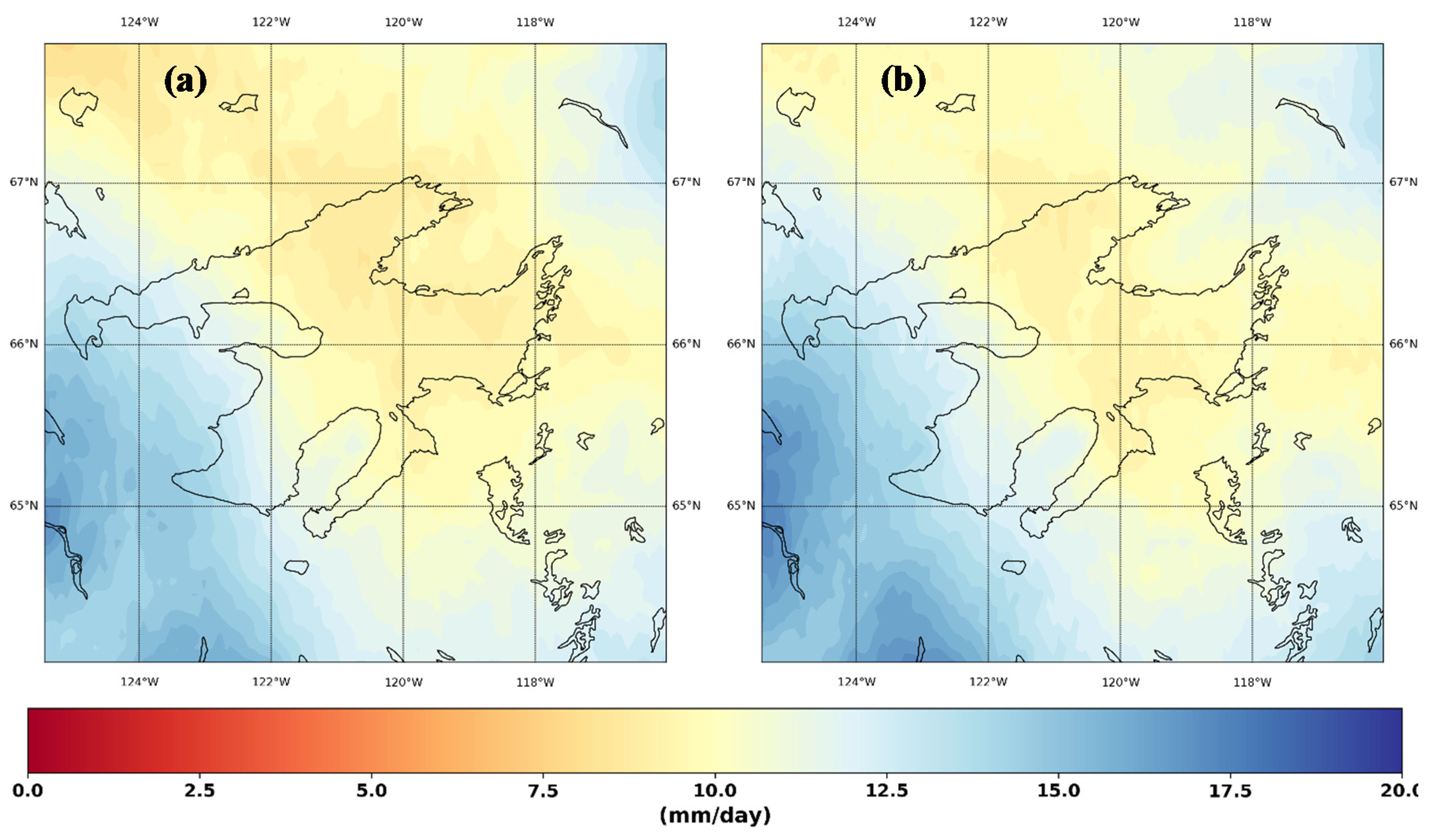
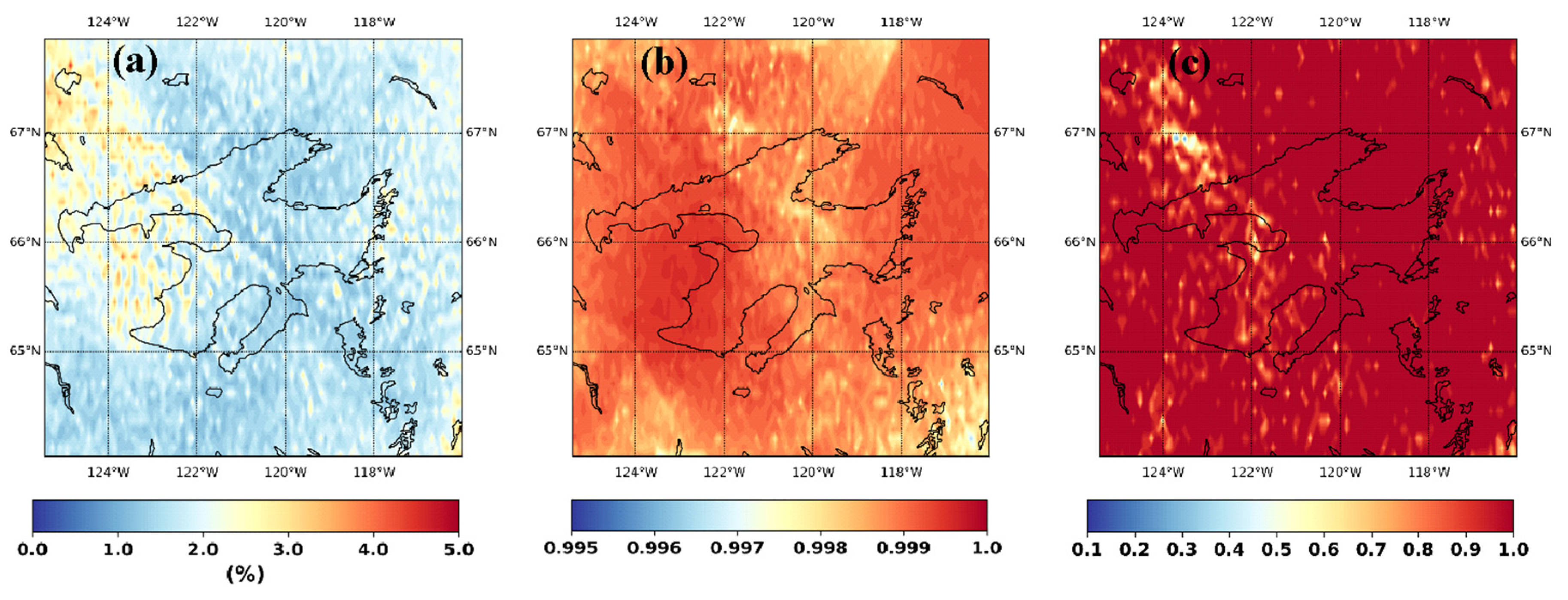
Figure 7 shows the temporal mean of observed (Figure 7a) and downscaled (Figure 7b) annual maximum precipitation. The regional patterns are well captured by the model. The observed pattern of high rainfall in the southwestern high region with orographic influences and the low rainfall over the lake is captured by the model. While more work is required to understand the performance of structural loss training of climate model outputs in different geographic contexts, the results here show that different processes are captured that yield more accurate overall output products. This is evident in the error diagnostics of the downscaling performance outlined in Figure 8. For the temporal mean absolute percent error (Figure 8a), the maximum error is around 5%, however, this error is mostly confined to the north-western part of the domain. We think this is due to the low observed rainfall without any special features in the models (which can again be attributed to the absence of orographic or land cover features) in this region attributed to this high percent error. Figure 8b shows the temporal correlation between the observed and downscaled precipitation. The minimum correlation is 0.995, which is well beyond the acceptable limit. However, interestingly, the correlation values show geometrical rectilinear orientation. We hypothesized that this is an artifact of the convolution filters used in the generator for downscaling, thus this result should be interpreted with caution. Calculating p-values for the Kolmogorov-Smirnov test for equivalency of temporal distribution of observed and downscaled annual maximum (Figure 8c) indicates that we cannot reject the equivalency of the distributions between the observed and downscaled (null hypothesis) at 90% confidence limit.
Table 3 shows the performance of different models and loss functions. The generative adversarial network is compared against the model trained using traditional mean absolute error and another network with principal component mapping. The performance functions are mean absolute error (MAE), NS coefficient, correlation coefficient, and p-value of the two sample KS tests. In all the performance measures the performance of GAN is superior followed by MAE based model. PCA based model performed poorly compared to the other model. However, all models performed reasonably well.
4. Conclusions
To our knowledge, this is the first attempt to downscale spatial fields of climate variables using a CNN with adversarial training. The major conclusions from our study are summarized below.
- Our framework can utilize diverse information present in different AOGCM simulations to create a spatially coherent field similar to observational data. The approach is similar in spirit to reliability ensemble averaging (REA) proposed by [75], within a CNN and adversarial training context.
- The MSSIM index allowed us to get an insight into the model’s regional characteristics and suggest relying solely on point-based error functions that are widely used in statistical downscaling and may not be enough to simulate regional characteristics of precipitation variables reliably.
- Further use of total loss function, which is a combination of adversarial, content, and structural loss within a CNN-based downscaling method, may lead to higher quality downscaled products.
- The adversarial loss can provide a meaningful gradient to weight optimization when traditional loss functions fail in near convergence variabilities.
These results hold considerable potential for fields investigating climate change impacts and climate processes. In many sectors, the scale mismatch between AOGCMs and spatial scales at the level of impacts (e.g., hydrological, ecological, economic) makes studying direct linkages and outcomes of climate models difficult. Downscaling methods in general help to bridge this divide by making climate model information more meaningful and useful for scientists working across disciplines at more localized geographic scales. Our analysis shows that incorporating the structure into the training of CNN-based statistical downscaling models reproduces observational gridded data for annual daily maximum rainfall in northern Canada, where station observational data are sparse and where climate change information is greatly needed. Further work developing and evaluating the CliGAN modeling framework in different geographic and thematic contexts is needed to realize the benefits to the wider scientific community.
Author Contributions
Conceptualization, C.C. and C.R.; methodology C.C. and C.R.; software, C.C. and C.R.; validation, C.C. and C.R.; formal analysis, C.C. and C.R.; investigation, C.C. and C.R.; resources, C.C. and C.R.; data curation, C.C. and C.R.; writing—original draft preparation, C.C. and C.R.; writing—review and editing, C.C. and C.R.; visualization, C.C. and C.R.; supervision, C.R.; project administration, C.R.; funding acquisition, C.R. All authors have read and agreed to the published version of the manuscript.
Funding
This work was funded in part by the Global Water Futures research program.
Conflicts of Interest
The authors declare that there is no competing interest.
Availability of Data and Material
Any data that support the findings of this study, not already publicly available, are available from the corresponding author, C. Chaudhuri, upon reasonable request.
Code Availability
The custom code used in this study, not already publicly available, are available from the corresponding author, C. Chaudhuri, upon reasonable request.
References
- Tryhorn, L.; DeGaetano, A. A comparison of techniques for downscaling extreme precipitation over the Northeastern United States. Int. J. Clim. 2011, 31, 1975–1989. [Google Scholar] [CrossRef]
- Chaudhuri, C.; Srivastava, R.; Srivastava, R. A novel approach for statistical downscaling of future precipitation over the Indo-Gangetic Basin. J. Hydrol. 2017, 547, 21–38. [Google Scholar] [CrossRef]
- Shi, X.; Chen, Z.; Wang, H.; Yeung, D.-Y.; Wong, W.; Woo, W. Convolutional LSTM Network: A Machine Learning Approach for Precipitation Nowcasting. Adv. Neural Inf. Process. Syst. 2015, 28, 802–810. [Google Scholar]
- Plouffe, C.C.; Robertson, C.; Chandrapala, L. Comparing interpolation techniques for monthly rainfall mapping using multiple evaluation criteria and auxiliary data sources: A case study of Sri Lanka. Environ. Model. Softw. 2015, 67, 57–71. [Google Scholar] [CrossRef]
- IPCC. Climate Change 2007: Impacts, Adaptation and Vulnerability. Contribution of Working Group II to the Fourth Assessment Report of the Intergovernmental Panel on Climate Change; Parry, M.L., Canziani, O.F., Palutikof, J.P., van der Linden, P.J., Hanson, C.E., Eds.; Cambridge University Press: Cambridge, UK, 2007; 976p. [Google Scholar]
- Prudhomme, C.; Jakob, D.; Svensson, C. Uncertainty and climate change impact on the flood regime of small uk catchments. J. Hydrol. 2003, 277, 1–23. [Google Scholar] [CrossRef]
- Smith, R.L.; Tebaldi, C.; Nychka, D.; Mearns, L.O. Bayesian modeling of uncertainty in ensembles of climate models. J. Am. Stat. Assoc. 2009, 104, 97–116. [Google Scholar] [CrossRef]
- Randall, D.; Wood, R.; Bony, S.; Colman, R.; Fichefet, T.; Fyfe, J.; Kattsov, V.; Pitman, A.; Shukla, J.; Srinivasan, J.; et al. Cilmate models and their evaluation. In Climate Change 2007: The Physical Science Basis, in Contribution of Working Group I to the Fourth Assessment Report of the Intergovernmental Panel on Climate Change; Solomon, S., Qin, D., Manning, M., Chen, Z., Marquis, M., Averyt, K., Tignor, M., Miller, H., Eds.; Cambridge University Press: Cambridge, UK; New York, NY, USA, 2007. [Google Scholar]
- Hughes, J.P.; Guttorp, P. A class of stochastic models for relating synoptic atmospheric patterns to regional hydrologic phenomena. Water Resour. Res. 1994, 30, 1535–1546. [Google Scholar] [CrossRef]
- Widmann, M.; Bretherton, C.S.; Salathé, E.P., Jr. Statistical precipitation downscaling over the north-western united states using numerically simulated precipitation as a predictor. J. Clim. 2003, 16, 799–816. [Google Scholar] [CrossRef]
- Knutti, R.; Furrer, R.; Tebaldi, C.; Cermak, J.; Meehl, G.A. Challenges in Combining Projections from Multiple Climate Models. J. Clim. 2010, 23, 2739–2758. [Google Scholar] [CrossRef] [Green Version]
- Trigo, R.M.; Palutikof, J.P. Precipitation scenarios over iberia: A comparison between direct gcm output and different downscaling techniques. J. Clim. 2001, 14, 4422–4446. [Google Scholar] [CrossRef]
- Brissette, F.; Khalili, M.; Leconte, R. Efficient stochastic generation of multisite synthetic precipitation data. J. Hydrol. 2007, 345, 121–133. [Google Scholar] [CrossRef]
- Maurer, E.P. Uncertainty in hydrologic impacts of climate change in the Sierra Nevada, California under two emissions scenarios. Clim. Chang. 2007, 82, 309–325. [Google Scholar] [CrossRef] [Green Version]
- Trzaska, S.; Schnarr, E. A Review of Downscaling Methods for Climate Change Projections; CIESIN, the Center for International Earth Science Information Network, Columbia University, Based at Columbia’s Lamont campus in Palisades: New York, NY, USA, 2014. [Google Scholar]
- Maraun, D.; Wetterhall, F.; Ireson, A.M.; Chandler, R.E.; Kendon, E.J.; Widmann, M.; Brienen, S.; Rust, H.W.; Sauter, T.; Themeßl, M.; et al. Precipitation downscaling under climate change: Recent developments to bridge the gap between dynamical models and the end user. Rev. Geophys. 2010, 48, RG3003. [Google Scholar] [CrossRef]
- Hewitson, B.; Crane, R.G. Crane Regional-scale climate prediction from the GISS GCM. Palaeogeogr. Palaeoclim. Palaeoecol. 1992, 97, 249–267. [Google Scholar] [CrossRef]
- Dibike, Y.B.; Coulibaly, P. Hydrologic impact of climate change in the Saguenay watershed: Comparison of downscaling methods and hydrologic models. J. Hydrol. 2005, 307, 145–163. [Google Scholar] [CrossRef]
- Murphy, J.M.; Sexton, D.; Barnett, D.N.; Jones, G.S.; Webb, M.J.; Collins, M.; Stainforth, D.A. Quantifying uncertainties in climate change from a large ensemble of general circulation model predictions. Nature 2004, 430, 768–772. [Google Scholar] [CrossRef]
- Wilby, R.L.; Harris, I. A framework for assessing uncertainties in climate change impacts: Low-flow scenarios for the river thames, UK. Water Resour. Res. 2006, 42, W02419. [Google Scholar] [CrossRef]
- Katz, R.W.; Parlange, M.B. Mixtures of stochastic processes: Applications to statistical downscaling. Clim. Res. 1996, 7, 185–193. [Google Scholar] [CrossRef] [Green Version]
- Richardson, C.W. Stochastic simulation of daily precipitation, temperature, and solar radiation. Water Resour. Res. 1981, 17, 182–190. [Google Scholar] [CrossRef]
- Kuchar, L. Using wgenk to generate synthetic daily weather data for modelling of agricultural processes. Math. Comput. Simul. 2004, 17, 69–75. [Google Scholar] [CrossRef]
- Schoof, J.T.; Arguez, A.; Brolley, J.; O’Brien, J. A new weather generator based on spectral properties of surface air temperatures. Agric. For. Meteorol. 2005, 135, 241–251. [Google Scholar] [CrossRef]
- Hanson, C.L.; Johnson, G.L. Gem (generation of weather elements for multiple applications): Its application in areas of complex terrain. Hydrol. Water Resour. Ecol. Headwaters 1998, 248, 27–32. [Google Scholar]
- Soltani, A.; Hoogenboom, G. A statistical comparison of the stochastic weather generators wgen and simmeteo. Clim. Res. 2003, 24, 215–230. [Google Scholar] [CrossRef] [Green Version]
- Semenov, M.A.; Barrow, E.M. Use of a stochastic weather generator in the development of climate change scenarios. Clim. Chang. 1997, 35, 397–414. [Google Scholar] [CrossRef]
- Wilks, D.S.; Wilby, R.L. The weather generation game: A review of stochastic weather models. Prog. Phys. Geogr. 1999, 23, 329–357. [Google Scholar] [CrossRef]
- Sharif, M.; Burn, D.H. Simulating climate change scenarios using an improved k-nearest neighbor model. J. Hydrol. 2006, 325, 179–196. [Google Scholar] [CrossRef]
- Brandsma, T.; Buishand, T.A. Buishand Simulation of extreme precipitation in the rhine basin by nearest-neighbour resampling. Hydrol. Earth Syst. Sci. 1998, 325, 195–209. [Google Scholar] [CrossRef]
- Yates, D.; Gangopadhyay, S.; Rajagopalan, B.; Strzepek, K. A technique for generating regional climate scenarios using a nearest-neighbour algorithm. Water Resour. Res. 2003, 39, 1199–1213. [Google Scholar] [CrossRef] [Green Version]
- Brown, B.G.; Katz, R.W. Regional analysis of temperature extremes: Spatial analog for climate change? J. Clim. 1995, 8, 108–119. [Google Scholar] [CrossRef] [Green Version]
- Crane, R.G.; Hewitson, B.C. Doubled co2 precipitation changes for the susquehanna basin: Down-scaling from the genesis general circulation model. Int. J. Climatol. 1998, 18, 65–76. [Google Scholar] [CrossRef]
- Cannon, A.J.; Whitfield, P.H. Downscaling recent streamflow conditions in British Columbia. Canada using ensemble neural network models. J. Hydrol. 2020, 259, 136–151. [Google Scholar] [CrossRef]
- Wilby, R.L.; Dawson, C.; Barrow, E. Sdsm—A decision support tool for the assessment of regional climate change impacts. Environ. Model. Softw. 2002, 17, 147–159. [Google Scholar] [CrossRef]
- Tripathi, S.; Srinivas, V.V.; Nanjundiah, R.S. Downscaling of precipitation for climate change scenarios: A support vector machine approach. J. Hydrol. 2006, 330, 621–640. [Google Scholar] [CrossRef]
- Zorita, E.; von Storch, H. The analog method—A simple statistical downscaling technique: Comparison with more complicated methods. J. Clim. 1999, 12, 2474–2489. [Google Scholar] [CrossRef]
- Wilby, R.L.; Hassan, H.; Hanaki, K. Statistical downscaling of hydrometeorological variables using general circulation model output. J. Hydrol. 1998, 205, 1–19. [Google Scholar] [CrossRef]
- Gutierrez, J.M.; Cofiño, A.S.; Cano, R.; Rodríguez, M.A. Clustering methods for statistical downscaling in short-range weather forecasts. Mon. Weather Rev. 2004, 132, 2169–2183. [Google Scholar] [CrossRef]
- Haylock, M.R.; Cawley, G.C.; Harpham, C.; Wilby, R.L.; Goodess, C.M. Downscaling heavy precipitation over the United Kingdom: A comparison of dynamical and statistical methods and their future scenarios. Int. J. Climatol. 2006, 26, 1397–1415. [Google Scholar] [CrossRef]
- Anh, D.T.; Van, S.P.; Dang, T.D.; Hoang, L.P. Downscaling rainfall using deep learning long short-term memory and feedforward neural network. Int. J. Clim. 2019, 39, 4170–4188. [Google Scholar] [CrossRef]
- LeCun, Y.; Bengio, Y. Convolutional networks for images, speech, and time series. In The Handbook of Brain Theory and Neural Networks; Arbib, M.A., Ed.; MIT Press: Cambridge, MA, USA, 1998; pp. 255–258. [Google Scholar]
- Krizhevsky, A.; Sutskever, I.; Hinton, G.E. ImageNet classification with deep convolutional neural networks. In Advances in Neural Information Processing Systems, Proceedings of the 25th International Conference on Neural Information Processing Systems—Volume 1; ACM: New York, NY, USA, 2012; pp. 1097–1105. [Google Scholar]
- Ronneberger, O.; Fischer, P.; Brox, T. U-net: Convolutional networks for biomedical image segmentation. In International Conference on Medical Image Computing and Computer-Assisted Intervention; Springer: Berlin/Heidelberg, Germany, 2015; pp. 234–241. [Google Scholar]
- Wang, Q.; Yuan, Z.; Du, Q.; Li, X. GETNET: A General End-to-End 2-D CNN Framework for Hyperspectral Image Change Detection. IEEE Trans. Geosci. Remote Sens. 2019, 57, 3–13. [Google Scholar] [CrossRef] [Green Version]
- Dong, C.; Loy, C.C.; He, K.; Tang, X. Learning a Deep Convolutional Network for Image Super-Resolution. In Computer Vision—ECCV 2014; Fleet, D., Pajdla, T., Schiele, B., Tuytelaars, T., Eds.; Lecture Notes in Computer Science; Springer: Cham, Switzerland, 2014; Volume 8692. [Google Scholar]
- Hashmi, M.Z.; Shamseldin, A.Y.; Melville, B.W. Statistical downscaling of precipitation: State-of-the-art and application of bayesian multi-model approach for uncertainty assessment. Hydrol. Earth Syst. Sci. Discuss. 2009, 6, 6535–6579. [Google Scholar] [CrossRef]
- Benestad, R.E. Downscaling precipitation extremes. Theor. Appl. Clim. 2010, 100, 1–21. [Google Scholar] [CrossRef] [Green Version]
- Wilks, D.S. Statistical Methods in the Atmospheric Sciences; Academic Press: San Diego, CA, USA, 1995; 467p. [Google Scholar]
- Sungkawa, I.; Rahayu, A. Extreme Rainfall Prediction using Bayesian Quantile Regression in Statistical Downscaling Modeling. Procedia Comput. Sci. 2019, 157, 406–413. [Google Scholar] [CrossRef]
- Zorzetto, E.; Marani, M. Extreme value metastatistical analysis of remotely sensed rainfall in ungauged areas: Spatial downscaling and error modelling. Adv. Water Resour. 2020, 135, 103483. [Google Scholar] [CrossRef]
- Vandal, T.; Kodra, E.; Ganguly, S.; Michaelis, A.; Nemani, R.; Ganguly, A.R. Deepsd: Generating high resolution climate change projections through single image super-resolution. In Proceedings of the 23rd ACM Sigkdd International Conference on Knowledge Discovery and Data Mining, Halifax, NS, Canada, 13–17 August 2017; pp. 1663–1672. [Google Scholar]
- Cheng, J.; Kuang, Q.; Shen, C.; Liu, J.; Tan, X.; Liu, W. ResLap: Generating High-Resolution Climate Prediction through Image Super-Resolution. IEEE Access 2020, 8, 39623–39634. [Google Scholar] [CrossRef]
- Onishi, R.; Sugiyama, D.; Matsuda, K. Super-Resolution Simulation for Real-Time Prediction of Urban Micrometeorology. SOLA 2019, 15, 178–182. [Google Scholar] [CrossRef] [Green Version]
- Ji, Y.; Zhi, X.; Tian, Y.; Peng, T.; Huo, Z.; Ji, L. Downscaling of Precipitation Forecasts Based on Single Image Super-Resolution. In EGU General Assembly EGU General Assembly Conference Abstracts; EGU2020-8533; European Geophysical Union General Assembly: Vienna, Austria, 2020. [Google Scholar] [CrossRef]
- Niu, B.; Wen, W.; Ren, W.; Zhang, X.; Yang, L.; Wang, S.; Zhang, K.; Cao, X.; Shen, H. Single Image Super-Resolution via a Holistic Attention Network. arXiv 2020, arXiv:2008.08767. [Google Scholar]
- Ai, W.; Tu, X.; Cheng, S.; Xie, M. Single Image Super-Resolution via Residual Neuron Attention Networks. arXiv 2020, arXiv:2005.10455. [Google Scholar]
- Goodfellow, I.; Pouget-Abadie, J.; Mirza, M.; Xu, B.; Warde-Farley, D.; Ozair, S.; Courville, A.; Bengio, Y. Generative adversarial nets. In Advances in Neural Information Processing Systems (NIPS), Proceedings of the 27th International Conference on Neural Information Processing Systems—Volume 2; ACM: New York, NY, USA, 2014; pp. 2672–2680. [Google Scholar]
- Stengel, K.; Glaws, A.; Hettinger, D.; King, R.N. Adversarial super-resolution of climatological wind and solar data. Proc. Natl. Acad. Sci. USA 2020, 117, 16805–16815. [Google Scholar] [CrossRef]
- Lantz, T.C.; Kokelj, S.V. Increasing rates of retrogressive thaw slump activity in the Mackenzie Delta region, N.W.T., Canada. Geophys. Res. Lett. 2008, 35. [Google Scholar] [CrossRef]
- Wilcox, E.J.; Keim, D.; De Jong, T.; Walker, B.; Sonnentag, O.; Sniderhan, A.E.; Mann, P.; Marsh, P. Tundra shrub expansion may amplify permafrost thaw by advancing snowmelt timing. Arct. Sci. 2019, 5, 202–217. [Google Scholar] [CrossRef] [Green Version]
- Quinton, W.; Hayashi, M.; Chasmer, L. Permafrost-thaw-induced land-cover change in the Canadian subarctic: Implications for water resources. Hydrol. Process. 2011, 25, 152–158. [Google Scholar] [CrossRef]
- Vors, L.S.; Boyce, M.S. Global declines of caribou and reindeer. Glob. Chang. Biol. 2009, 15, 2626–2633. [Google Scholar] [CrossRef]
- Ford, J.D.; McDowell, G.; Pearce, T. The adaptation challenge in the Arctic. Nat. Clim. Chang. 2015, 5, 1046–1053. [Google Scholar] [CrossRef]
- Hutchinson, M.F.; McKenney, D.W.; Lawrence, K.; Pedlar, J.H.; Hopkinson, R.F.; Milewska, E.; Papadopol, P. Development and Testing of Canada-Wide Interpolated Spatial Models of Daily Minimum–Maximum Temperature and Precipitation for 1961–2003. J. Appl. Meteorol. Clim. 2009, 48, 725–741. [Google Scholar] [CrossRef]
- Wetterhall, F.; Halldin, S.; Xu, C.-Y. Statistical precipitation downscaling in central sweden with the analogue method. J. Hydrol. 2005, 306, 174–190. [Google Scholar] [CrossRef]
- Arjovsky, M.; Chintala, S.; Bottou, L. Wasserstein gan. arXiv 2017, arXiv:1701.07875. [Google Scholar]
- Villani, C. Optimal Transport: Old and New; Springer Science & Business Media: Berlin/Heidelberg, Germany, 2008; Volume 338. [Google Scholar]
- Wang, Z.; Simoncelli, E.P.; Bovik, A.C. Multiscale structural similarity for image quality assessment. In Proceedings of the Thrity-Seventh Asilomar Conference on Signals, Systems & Computers, Pacific Grove, CA, USA, 9–12 November2003; Volume 2, pp. 1398–1402. [Google Scholar]
- Kingma, D.P.; Ba, J. Adam: A Method for Stochastic Optimization. In Proceedings of the 3rd International Conference on Learning Representations (ICLR), San Diego, CA, USA, 7–9 May 2015. [Google Scholar]
- Ruder, S. An overview of gradient descent optimization algorithms. arXiv 2016, arXiv:1609.04747. [Google Scholar]
- Zeiler, M.D. Adadelta: An Adaptive Learning Rate Method. arXiv 2012, arXiv:1212.5701. [Google Scholar]
- Chen, H.; Sun, J.; Chen, X. Projection and uncertainty analysis of global precipitation-related extremes using CMIP5 models. Int. J. Clim. 2014, 34, 2730–2748. [Google Scholar] [CrossRef]
- Manzanas, R.; Lucero, A.; Weisheimer, A.; Gutiérrez, J.M. Can bias correction and statistical downscaling methods improve the skill of seasonal precipitation forecasts? Clim. Dyn. 2018, 50, 1161–1176. [Google Scholar] [CrossRef] [Green Version]
- Giorgi, F.; O Mearns, L. Probability of regional climate change calculated using the reliability ensemble averaging (REA) method. Geophys. Res. Lett. 2003, 30. [Google Scholar] [CrossRef]
- Frei, C.; Schöll, R.; Fukutome, S.; Schmidli, J.; Vidale, P.L. Future change of precipitation extremes in Europe: Intercomparison of scenarios from regional climate models. J. Geophys. Res. 2006, 111, D06105. [Google Scholar] [CrossRef] [Green Version]
- Hundecha, Y.; Bárdossy, A. Statistical downscaling of extremes of daily precipitation and temperature and construction of their future scenarios. Int. J. Climatol. 2008, 28, 589–610. [Google Scholar] [CrossRef]
Figure 1.
Study domain over the Tsa Tue Bio-reserve, located in Northwest Territories, Canada. In the inset, the location is shown in the box in the perspective of the entire Canada. The basemap is downloaded from ESRI© using opensource python package.
Figure 1.
Study domain over the Tsa Tue Bio-reserve, located in Northwest Territories, Canada. In the inset, the location is shown in the box in the perspective of the entire Canada. The basemap is downloaded from ESRI© using opensource python package.

Figure 2.
Schematic of the generative adversarial network.

Figure 3.
Temporal median of AOGCM annual maximum precipitation of (a) BCC ESM, (b) CAN ESM5, (c) CESM2, (d) CNRM CM6.1, (e) CNRM ESM2, (f) GFDL CM4, (g) HAD GEM3, (h) MRI, and (i) UK ESM1.
Figure 3.
Temporal median of AOGCM annual maximum precipitation of (a) BCC ESM, (b) CAN ESM5, (c) CESM2, (d) CNRM CM6.1, (e) CNRM ESM2, (f) GFDL CM4, (g) HAD GEM3, (h) MRI, and (i) UK ESM1.

Figure 4.
Different loss functions, used for training and their training and testing error.

Figure 5.
(a) Total loss of training, (b) content loss, (c) structural loss, (d) adversarial loss, (e) discriminator loss, (f) mean absolute error of the training.
Figure 5.
(a) Total loss of training, (b) content loss, (c) structural loss, (d) adversarial loss, (e) discriminator loss, (f) mean absolute error of the training.

Figure 6.
(a) Total loss of training, (b) content loss, (c) structural loss, (d) adversarial loss, (e) discriminator loss, (f) mean absolute error of the training.
Figure 6.
(a) Total loss of training, (b) content loss, (c) structural loss, (d) adversarial loss, (e) discriminator loss, (f) mean absolute error of the training.

Figure 7.
The temporal median of annual maximum precipitation (a) observed and (b) simulated.

Figure 8.
Performance of the downscaling (a) mean absolute percentage error, (b) temporal correlation, and (c) P-value for Kolmogorov-Smirnov test of temporal distribution equivalency.
Figure 8.
Performance of the downscaling (a) mean absolute percentage error, (b) temporal correlation, and (c) P-value for Kolmogorov-Smirnov test of temporal distribution equivalency.


Table 1.
Features of different input atmosphere–ocean global climate models (AOGCMs).
| AOGCM | Institution | Grid Type | Horizontal Dimension (Lon/Lat) | Vertical Levels |
|---|---|---|---|---|
| BCC ESM | Beijing Climate Center | T42 | 128 × 64 | 26 |
| CAN ESM5 | Canadian Centre for Climate Modelling and Analysis, Environment and Climate Change Canada | T63 | 128 × 64 | 49 |
| CESM2 | National Center for Atmospheric Research | 0.9 × 1.25 finite volume grid | 288 × 192 | 70 |
| CNRM CM6.1 | Centre National de Recherches Meteorologiques | T127 | 256 × 128 | 91 |
| CNRM ESM2 | Centre National de Recherches Meteorologiques | T127 | 256 × 128 | 91 |
| GFDL CM4 | Geophysical Fluid Dynamics Laboratory | C96 | 360 × 180 | 33 |
| HAD GEM3 | Met Office Hadley Centre | N96 | 192 × 144 | 85 |
| MRI | Meteorological Research Institute, Tsukuba, Ibaraki 305-0052, Japan | TL159 | 320 × 160 | 80 |
| UK ESM1 | Met Office Hadley Centre | N96 | 192 × 144 | 85 |
Table 2.
Performance of different objective functions for the model. The median of the last 50 iterations has been used to measure the performance.
Table 2.
Performance of different objective functions for the model. The median of the last 50 iterations has been used to measure the performance.
| Loss Combination | Content Loss | Structural Loss | ||
|---|---|---|---|---|
| Train | Test | Train | Test | |
| Adversarial + NS | 0.015 | 0.142 | 0.025 | 0.100 |
| Adversarial + MSSIM | 0.070 | 0.110 | 0.019 | 0.025 |
| NS + MSSIM | 0.011 | 0.774 | 0.024 | 0.283 |
| Adversarial + NS + MSSIM | 0.015 | 0.043 | 0.024 | 0.033 |
| Adversarial + NS + MSSIM LT | 0.011 | 0.020 | 0.021 | 0.017 |
Table 3.
Performance comparison of different downscaling models.
| Performance/Model | GAN | MAE | PCA |
|---|---|---|---|
| MAE | 1.71 | 1.85 | 2.7 |
| NS | 0.996 | 0.995 | 0.991 |
| Correlation | 0.9987 | 0.9986 | 0.995 |
| KS p-value | ~1−48 | ~1−25 | ~1−8 |
Publisher’s Note: MDPI stays neutral with regard to jurisdictional claims in published maps and institutional affiliations. |
© 2020 by the authors. Licensee MDPI, Basel, Switzerland. This article is an open access article distributed under the terms and conditions of the Creative Commons Attribution (CC BY) license (http://creativecommons.org/licenses/by/4.0/).
Share and Cite
MDPI and ACS Style
Chaudhuri, C.; Robertson, C. CliGAN: A Structurally Sensitive Convolutional Neural Network Model for Statistical Downscaling of Precipitation from Multi-Model Ensembles. Water 2020, 12, 3353. https://doi.org/10.3390/w12123353
AMA Style
Chaudhuri C, Robertson C. CliGAN: A Structurally Sensitive Convolutional Neural Network Model for Statistical Downscaling of Precipitation from Multi-Model Ensembles. Water. 2020; 12(12):3353. https://doi.org/10.3390/w12123353
Chicago/Turabian StyleChaudhuri, Chiranjib, and Colin Robertson. 2020. "CliGAN: A Structurally Sensitive Convolutional Neural Network Model for Statistical Downscaling of Precipitation from Multi-Model Ensembles" Water 12, no. 12: 3353. https://doi.org/10.3390/w12123353
Note that from the first issue of 2016, this journal uses article numbers instead of page numbers. See further details here.