Inventory and Connectivity Assessment of Wetlands in Northern Landscapes with a Depression-Based DEM Method


1
Department of Physical Geography, Stockholm University, SE-106 91 Stockholm, Sweden
2
Ecosystems and Environment Research Programme, and Helsinki Institute of Sustainability Science (HELSUS), Faculty of Biological and Environmental Sciences, University of Helsinki, FI-00014 Helsinki, Finland
3
Navarino Environmental Observatory, Costa Navarino, Navarino Dunes, 24001 Messinia, Greece
4
Department of Sustainable Development, Environmental Science and Engineering, KTH Royal Institute of Technology, SE-100 44 Stockholm, Sweden
*
Author to whom correspondence should be addressed.
Water 2020, 12(12), 3355; https://doi.org/10.3390/w12123355
Submission received: 18 September 2020
/
Revised: 19 November 2020
/
Accepted: 21 November 2020
/
Published: 30 November 2020
(This article belongs to the Special Issue Impact of Land-Use Changes on Surface Hydrology and Water Quality)
Abstract
:Wetlands, including peatlands, supply crucial ecosystem services such as water purification, carbon sequestration and regulation of hydrological and biogeochemical cycles. Peatlands are especially important as carbon sinks and stores because of the incomplete decomposition of vegetation within the peat. Good knowledge of individual wetlands exists locally, but information on how different wetland systems interact with their surroundings is lacking. In this study, the ability to use a depression-based digital elevation model (DEM) method to inventory wetlands in northern landscapes and assess their hydrological connectivity was investigated. The method consisted of three steps: (1) identification and mapping of wetlands, (2) identification of threshold values of minimum wetland size and depth, and (3) delineation of a defined coherent area of multiple wetlands with hydrological connectivity, called wetlandscape. The results showed that 64% of identified wetlands corresponded with an existing wetland map in the study area, but only 10% of the wetlands in the existing map were identified, with the F1 score being 17%. Therefore, the methodology cannot independently map wetlands and future research should be conducted in which additional data sources and mapping techniques are integrated. However, wetland connectivity could be mapped with the depression-based DEM methodology by utilising information on upstream and downstream wetland depressions, catchment boundaries and drainage flow paths. Knowledge about wetland connectivity is crucial for understanding how physical, biological and chemical materials are transported and distributed in the landscape, and thus also for resilience, management and protection of wetlandscapes.
1. Introduction
Wetlands play an important role in the world’s freshwater system [1]. As a result of changes in land and water use driven by humans and climate change, wetlands have declined globally [2,3]. According to Ramsar [4], 64% of the world’s wetlands disappeared in the 20th century, with 40% of them occurring in the last 50 years. Wetlands are crucial in supplying ecosystem services such as the regulation of hydrological cycles, including flood control [5], groundwater generation, soil moisture [6,7], purification of water [8] and regulation of biochemical cycles [9], and in supporting carbon sequestration [10] and biodiversity [11,12,13,14,15]. This potential to supply multiple ecosystem services makes wetlands relevant as nature-based solutions (NBS), with an ability to manage environmental, social and economic challenges [16] through nature [17]. There have been widespread calls for strategies to manage and sustain important wetland functions in northern landscapes [11,18,19,20,21,22,23].
In high-latitude northern landscapes, comprising Arctic, subarctic and northern boreal areas, approximately 60% of the surface is covered by freshwater systems, including wetlands [1]. Wetlands are an established concept but the specific definition varies, since wetlands are found in the area between terrestrial and aquatic systems [24]. Gunnarsson and Löfroth [25] defined wetlands as vegetation-covered water areas or land surfaces where water is close to, over or just below, the soil surface for most of the year [25].
According to several climate models, the greatest future warming will occur at high latitudes in the northern hemisphere [25,26,27]. In fact, significant warming in the climate of northern landscapes has been noted over the past 30 years [20]. This warming is causing the snowpack to melt during summer and recover less during winter, resulting in a loss of meltwater that feeds many wetlands, which may diminish or disappear [21]. Temperature rise also affects the water balance, due to higher evaporation rates and higher inputs of water to the landscape as a whole [21]. According to Land and Carson [22], there is a lack of knowledge of how future climate change will affect the functioning of northern wetland landscapes and thereby the people supported by these landscapes. Peatlands are the main type of wetland in northern landscapes and, although they cover less than 3% of the world’s surface, they hold about one-third of global soil carbon and are the largest natural source of methane to the atmosphere [28]. Peat consists of organic matter accumulated in waterlogged conditions, which leads to an anaerobic environment and slow decomposition rate [29]. The loss of water and permafrost in peatlands driven by global changes has impacts on peatland carbon storage and dynamics, potentially moving peatlands from being a sink of carbon to becoming a source of carbon [30,31].
Although northern wetland landscapes are key to achieving sustainable development in the region [22], the spatial loss of wetlands is unknown, since many parts of the region lack the inventories needed to estimate wetland loss over time [32]. Good knowledge of individual wetlands is available locally [33]. Wetland and peatland extent have been mapped with various remote sensing datasets and semi-automated land use/land cover classification approaches. The datasets typically used include optical satellite, aerial and drone images, which can capture spectral properties of vegetation and land cover, and satellite-based synthetic aperture radar data, which can capture differences in moisture, surface roughness and vegetation structure [34,35]. However, as trees cover many of northern wetland landscapes, remote sensing-based classifications often confuse peatlands with forests on mineral soil. Therefore, optical and radar data are often analysed together with topographic data derived e.g., from LIDAR-based digital elevation models (DEMs) [35]. It has also been shown that topographic data alone can model wet area extent accurately, for instance when using topographic indices such as topographic wetness and depth to water, which model how water flows in the landscape and where it possibly stays [36,37].
Wetlands are characterised by complex interconnected processes of fill and spill, leading to water fluctuations over the landscape [26]. These processes cause changes in hydrological connectivity, leading to transport of water, energy, material and organisms among elements of the hydrological cycle [27]. The flows of water and the inundation of wetlands vary spatially and temporally. Geographically isolated wetlands, which lack surface water connections, also affect the system connectivity by reducing the interconnection of the flows [26]. Hydrological connectivity has critical effects on wetland conditions, which in turn impacts upon the hydrological connectivity at landscape scale [26]. Based on the hydrological connectivity of multiple wetlands, Thorslund et al. [38] developed the “wetlandscape” concept, which links individual wetlands to the larger watershed scale by hydrological connectivity.
However, knowledge of how different wetland systems interact with their surroundings is lacking. Although previous studies have used technology to assess preferential water pathways in wetlands, such as dye tracer [39], computed tomography [40] and nuclear magnetic resonance [41], these methodologies are used at a small scale to understand the relationship between hydrological processes and soil properties. Few studies have focused on flow connectivity at a larger scale, based on field instrumentation, but still covering a relatively limited extent of the landscape [42]. Model frameworks have been developed recently to explore landscape permeability or dispersal characteristics within wetlands, but focusing on landscape connectivity for wildlife [43]. Existing models do not have the capacity to consider geometry or quantify subsurface connectivity in a wetlandscape perspective [32]. Comprehensive inventories of wetland areas would be useful in assessing the effectiveness of different regulatory and management activities, knowledge that could guide policymakers and stakeholders [22].
The aim of this study was to investigate the capability of a depression-based DEM method for mapping northern landscape wetlands and, in particular, to increase understanding of wetland dynamics through mapping hydrological connectivity among wetlands. Specific objectives were to: (1) identify wetland areas using a mapping technique based on DEM; (2) evaluate threshold values of size and depth to identify wetlands; and (3) assess the hydrological connectivity of wetlands between catchments. The method developed was based on the premise that surface depressions often give rise to temporary, seasonal or permanent wetlands, since runoff from upslope areas is retained at downslope sites within the landscape [44,45,46].
2. Material and Methods
2.1. Study Site
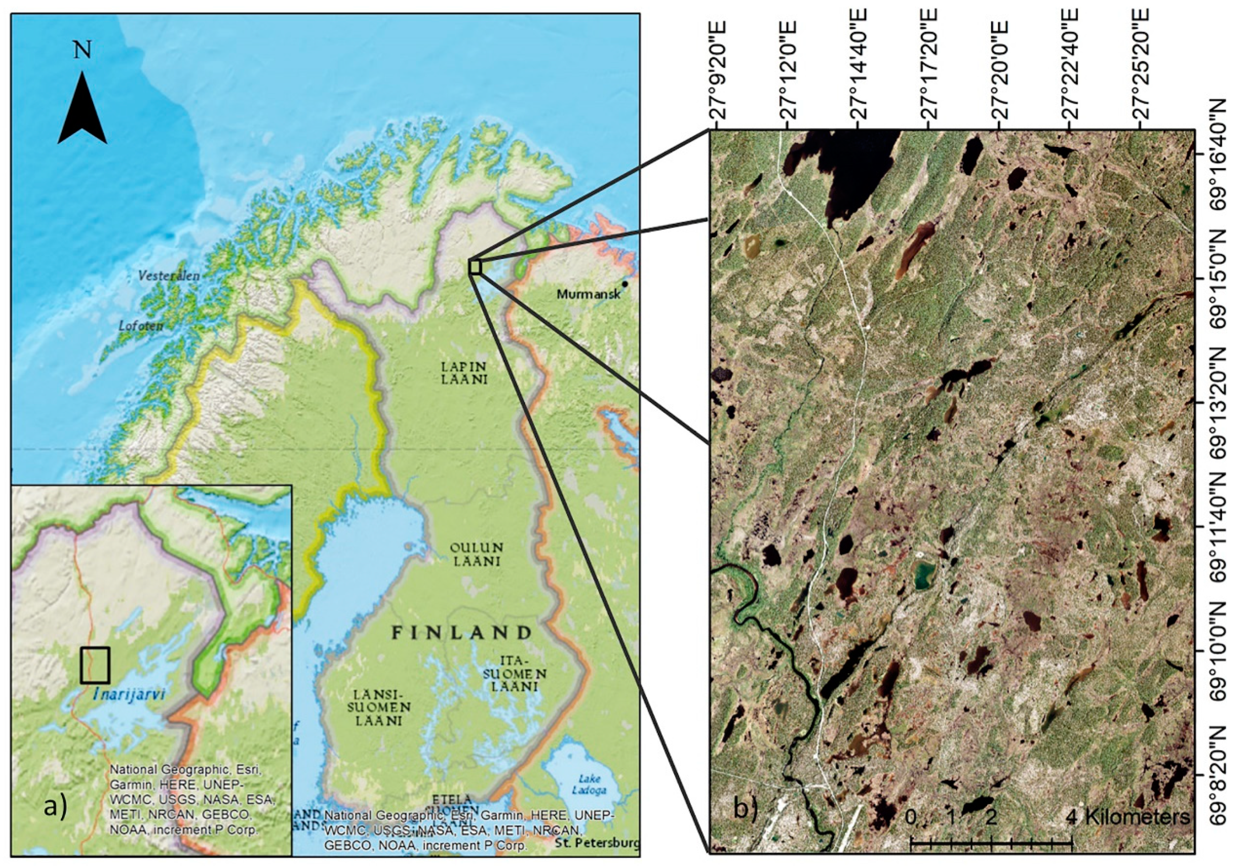
The study site was a 214 km2 area near the village of Kaamanen in the municipality of Inari in northern Finland (69°8.435′ N, 27°16.189′ E) (Figure 1). The region is located in the northern boreal vegetation zone and in the subarctic climate zone (Dfc zone in the Köppen climate classification system), which is characterised by a cold climate without dry seasons and cold summers [47]. The study site is adjacent to Lake Inari, the third largest lake in Finland (Figure 1) and just south of the Sammuttijänkä-Vaijoenjänkä mires, a Ramsar site. Based on data from the closest nearby weather station (Inari Ivalo airport; 68°36.65′ N, 27°24.833′ E) for the period 1981–2010, mean annual temperature at the site is −0.4 °C and mean annual precipitation is 472 mm [48]. There is no permafrost in the area, and the topography is flat, characterised by flat peatlands and some forested hills and esker ridges, with elevation varying between 138 and 242 m a.s.l. Managed pine (Pinus sylvestris) forests dominate the area, but birch (Betula pubescens) and mixed pine-birch forests are also present [49]. Lakes and ponds cover 8% of the study area, while approximately 36% is covered by peatlands, including both tree-covered and open peatlands.
2.2. Mapping Wetlands
The depression-based DEM method investigated for mapping wetlands and their hydrological connectivity included the following three steps: (1) identification and mapping of wetlands; (2) identification of threshold values; and (3) delineation of wetlandscapes using hydrological connectivity.
2.2.1. Data Acquisition and Pre-Processing
The data used consisted of a DEM, an aerial image and a topographic database managed by the National Land Survey (NLS) of Finland, which are freely available at https://tiedostopalvelu.maanmittauslaitos.fi/tp/kartta?lang=en. NLS produced the DEM from LIDAR data and manually inspected it using aerial image interpretation. The data had spatial resolution of 2 m × 2 m and vertical accuracy of 0.15–0.3 m, and were acquired on 12 July 2016. The NLS DEM was further pre-processed with a 3 × 3 cell moving window mean filter to remove artefacts which, unlike actual surface depressions, often have a more irregular shape and size and are shallower, and originate from construction operators when producing the DEM [50]. A four-band (blue, green, red, near infra-red) 0.5 m spatial resolution aerial image of the study area was acquired on 27 June 2016. The image was orthorectified by NLS and had positional accuracy of 0.5–2.0 m. The topographic database obtained included land cover information about lakes, streams and wetlands in a vector format and 1:10,000 scale. These terrain attributes were used as validation and comparison data specifically to identify threshold values, such as wetland minimum depth and size, to delineate wetlands.
2.2.2. Identification and Mapping of Wetlands
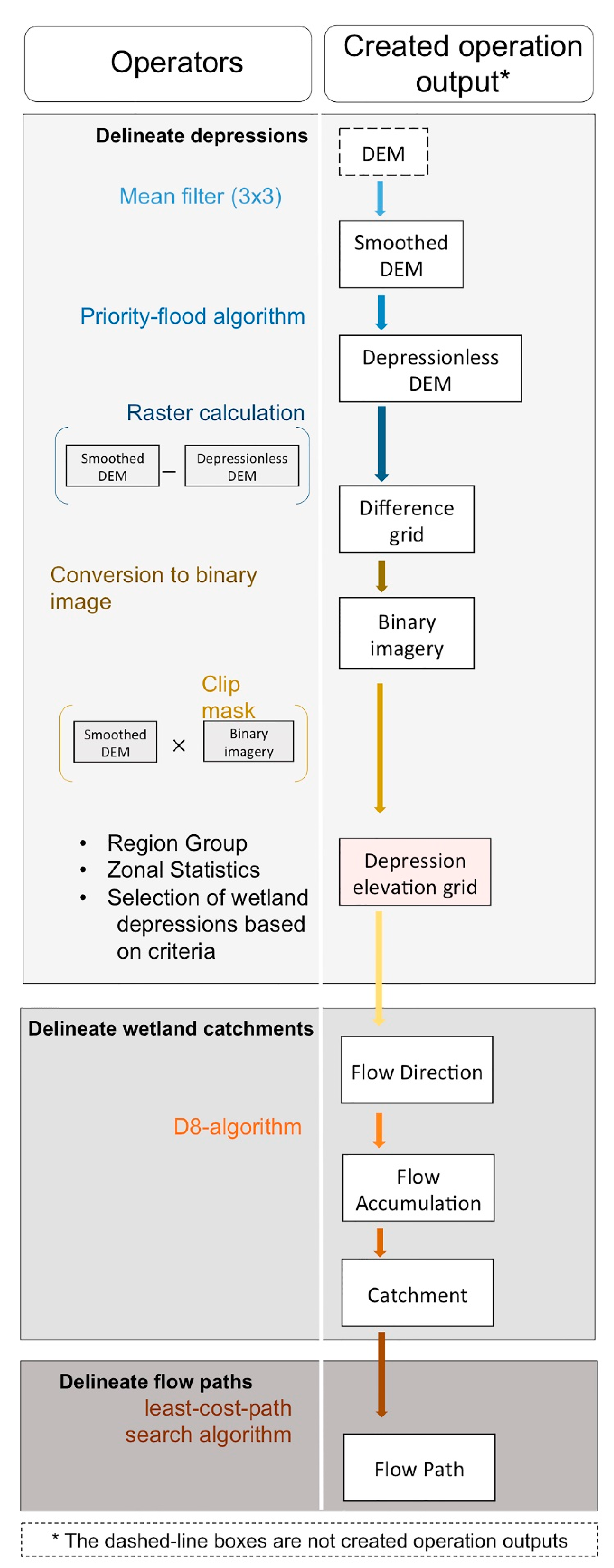
The procedure of delineating potential wetlands using depression-based DEM was done using an addition to the existing ArcGIS toolbox called Wetland Hydrology Analyst, developed by Wu and Lane [51], which is freely accessible for download at https://figshare.com/articles/software/Wetland_Hydrology_Analyst_Toolbox/8866025. The different steps followed in the modelling work in the toolbox are illustrated as a workflow in Figure 2, and described below.
Delineation of Wetlands
In the first modelling step, a depressionless DEM was generated by identifying and filling the depressions in the DEM. This task was performed using the priority-flood algorithm developed by Wang and Liu [52], where filling proceeds to the level where water would start to overflow from the perimeter. The geometrical boundary of the wetland was thereby defined by the “pond” created by flooding the depression. The filled depressions were then used as a template to subtract the depressions that led the defined threshold values, including minimum size and depth. This is a computationally more efficient procedure than searching for, identifying and selecting depressions from the original DEM [52]. In a second step, an elevation difference grid was obtained by subtracting the original DEM from the depressionless DEM, where each cell value represented the depression depth. In a third step, the difference grid was converted to a binary image where all cells with value greater than 0 (depressions) were set to 1 and all cells with 0 (non-depressions) were set to remain 0. In step four, the binary image was used as a template to subtract the original smoothed DEM data for the depression areas. In a fifth step, a region group algorithm was applied to the DEM subset, which is a method of connecting the continuous set of depression cells together, forming regions and naming them [53]. In step six, the zonal statistics of depressions were calculated from the input raster [54]. Once the grouping and statistics for each depression had been obtained, in step seven the potential wetlands were identified from the DEM subset using threshold values. Since depressions show many shapes and sizes in the landscape, defining the threshold values for minimum depression size and associated depth enabled depressions that are potential wetlands to be located. A separate vector file was obtained containing polygons with depressions that fulfilled the criteria, in other words potential wetlands.
Delineation of Wetland Catchments
Once the wetlands were defined, their corresponding potential catchment was delineated. This was done by first calculating the flow direction based on the DEM, where the flow direction from a cell was defined by its steepest downslope neighbour [55], i.e., the D8 algorithm by O’Callaghan and Mark [56]. All depressions that did not fulfil the threshold values were assumed to be filled, to prevent water from being trapped in these incorrect wetlands. The flow direction was used to obtain the flow accumulation, determined by the number of cells that flowed into each cell downstream [57], which in turn was used to delineate flow paths in the following step. Cells with high values are likely to represent channels where water will accumulate, whereas cells with low values are higher up and represent landforms such as ridges [57]. The wetland catchment was obtained by the surrounding cells with a flow direction towards the wetland.
Delineation of Drainage Flow Paths
The potential flow path is the path that water takes when a wetland is filled and water starts to spill out from the wetland as runoff. To obtain the flow path, the depressionless DEM was used together with the vector file of identified wetlands and a filling parameter, which was rainfall intensity. The rainfall intensity parameter only affected the time taken for each wetland to be filled in the model, the so-called ponding time, and not the actual flow path. The ponding time indicated the order in which a wetland was filled in relation to adjacent wetlands, which was used to determine the flow path. The rainfall intensity was assumed to be equally distributed over the study site, which meant that the value of rainfall intensity did not have an impact on the delineation of wetlands. The least-cost-path search algorithm was used to obtain the flow path that water takes from a wetland when it spills out [58]. The vector file was used to locate the centroid of each depression, which was used as the starting point for the least-cost-path search algorithm. The distance from the wetland centroid to its spilling point was later removed. The ponding time was calculated from the ratio between potential water storage of the wetland (maximum ponding volume before water spills out, determined through Equation (1), and catchment wetland area and rainfall intensity, determined according to Equation (2).
where V [m3] is potential water storage, n [-] is number of cells that fall within the depression, C [m] is elevation of the cell from which the water spills out, Zi [m] is the elevation of the grid cell and R [m] is the spatial resolution.
where T [h] is the ponding time, V [m3] is potential water storage, Ac [m2] is catchment wetland area and I [cm/h] is rainfall intensity.
2.2.3. Identification of Threshold Values
In order to identify potential wetlands using the model, the most representative thresholds of minimum wetland size and depth were (i) examined by first studying the output results from several model runs performed with varying threshold values randomly attributed, and (ii) compared with the NLS Finland map of wetlands in the study area. After initial parameter testing, in which the minimum wetland size varied from 50 m2 to 10,000 m2, the model was run with two values (minimum wetland sizes of 100 and 1000 m2) that showed correspondence with the previous mapping of wetlands by NLS Finland. Two minimum sizes were chosen so that comparison could be made between analysis that either included (minimum wetland size 100 m2) or excluded (minimum wetland size 1000 m2) small wetlands. Six values of minimum depth (0.1, 0.2, 0.3, 0.4, 0.5 and 0.6 m) were used to study the depth that showed the highest similarity with the existing mapping of wetlands by NLS Finland, resulting in 12 outputs. The coverage of potential wetlands obtained from each model run was compared against the NLS Finland map of wetlands and lakes in the study area [59]. Since identification of wetlands basically consists of finding depressions in the landscape, it is likely that wetlands will appear where lakes are located. However, the LIDAR technique used to obtain the DEM cannot penetrate water, which means that the water surface of lakes and ponds appeared as a solid surface when the model searched for depressions. Therefore, the wetlands that might coincide with lakes represented the volume that would be added if the lake were filled to the brim, before water poured out to a downstream depression. Based on the definition of wetland used in this study [25], the area that coincided with lakes was not included in wetland mapping.
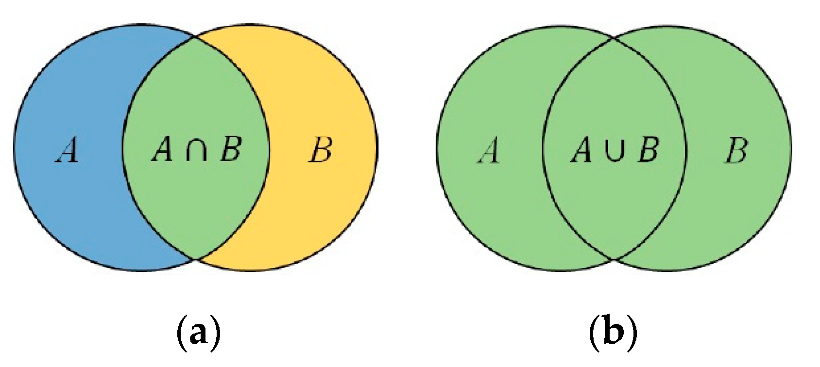
A comparison was made using Jaccard similarity index [60], a measurement of similarity, of how well the wetlands identified by the model coincided with those in existing maps created by NLS Finland. Jaccard similarity index is obtained by dividing the size of the intersection between two sets by the combined size of the same sets (Equation (3)), as illustrated in Figure 3.
where A is one set (here NLS Finland topographic database) and B another set (here wetlands identified by the model).
To further validate how accurately the modelled wetlands corresponded to wetlands mapped by NLS Finland, a confusion matrix was used. In addition, user accuracy (precision), producer accuracy (recall) and F1 score were calculated, using the following equations:
where TP is true positives, FP false positives and FN false negatives obtained from the confusion matrix.
2.2.4. Delineation of Wetlandscape Using Hydrological Connectivity
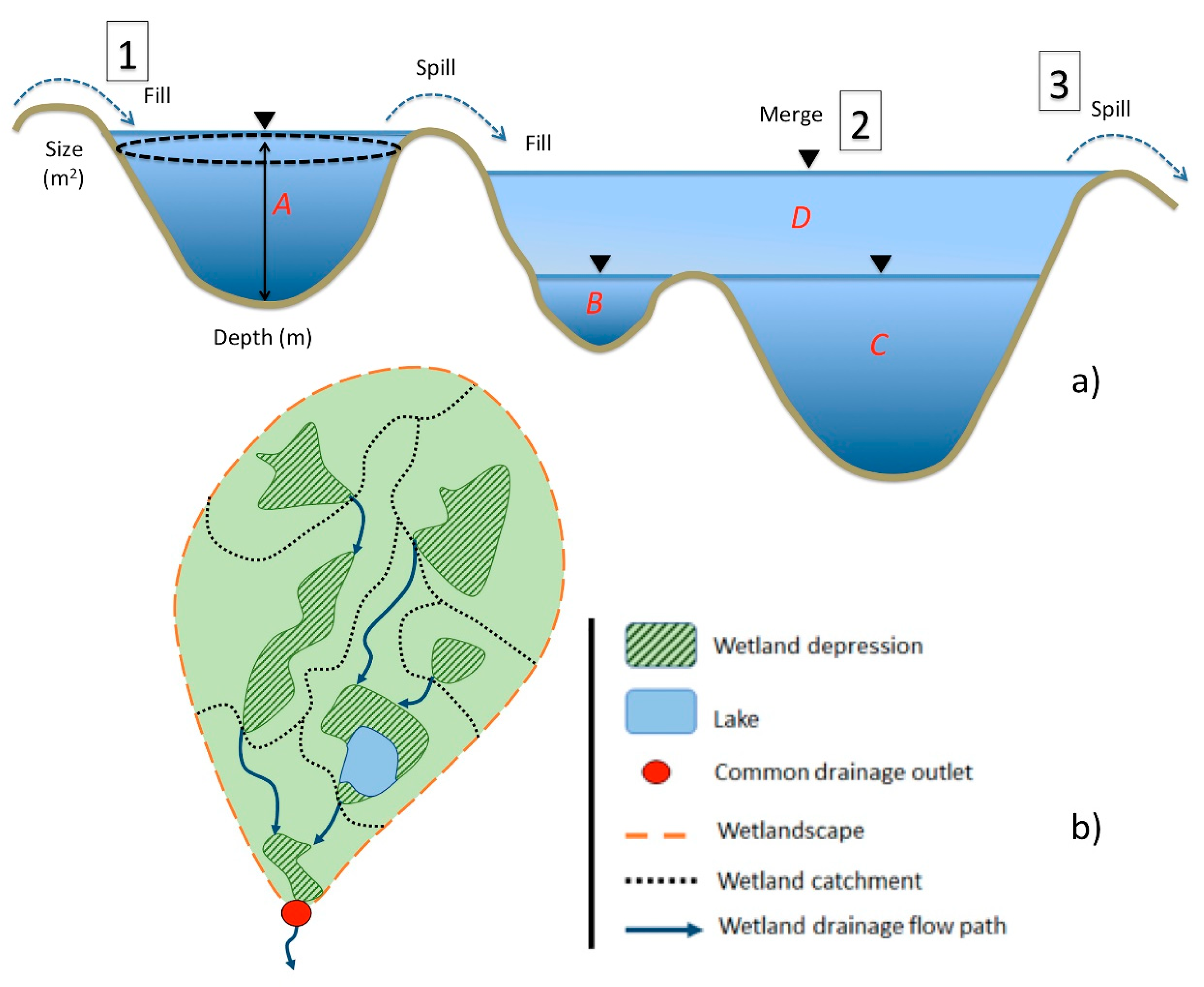
Surface depressions cause spatially varying and independently localised hydrological systems by trapping water, thereby breaking the connectivity in a landscape [61]. Since surface depressions can vary in size, they fill at different rates, affecting the hydrological connectivity by regulating the flow. Information on the filling-merging-spilling processes within a wetland is vital for characterising their hydrological connectivity [46]. When a wetland fills (step 1 in Figure 4a) with water and reaches its maximum storage, it can either merge (step 2 in Figure 4a) with an adjacent wetland or allow water to spill (step 3 in Figure 4a) to a downstream wetland (Figure 4b) [26].
In the methodology developed, the hydrological connectivity obtained by the delineated drainage flow paths represents the maximum water capacity of the system (i.e., maximum change over time), since the model fills the wetlands to the brim to produce drainage flow paths. The flow paths from each identified wetland together make up an interconnected set of drainage routes, where upstream wetlands drain to downstream wetlands. In this way, information on adjacent wetlands that are connected, and how, is obtained.
To validate the delineated drainage flow paths, stream waters mapped by NLS Finland were used for comparison. Since information about the spatial extent of each wetland within the catchment and the specific drainage flow path was acquired after running the model, the hydrologically coupled system and the total hydrological catchment were obtained. For each wetland identified, information on the wetland located downstream was used to track how the water flowed in the wetlandscape. Some wetlands did not have a direct drainage flow path connection to a downstream wetland, but information on the wetland located downstream was still obtained. The wetlandscape was determined by selecting the connected wetlands (located just upstream and releasing water to downstream wetlands, or located just downstream and receiving water from upstream wetlands), with their individual catchments (Figure 4). This information was obtained in the resulting file after executing the tool. The wetlandscape obtained was thereby a type of catchment or sub-catchment where all wetland catchments that had interconnections resulted in a watershed with a common drainage outlet. The delineation of the wetlandscape was not automated and involved manual tracing of the connections in the data.
3. Results
3.1. Identified Potential Wetlands
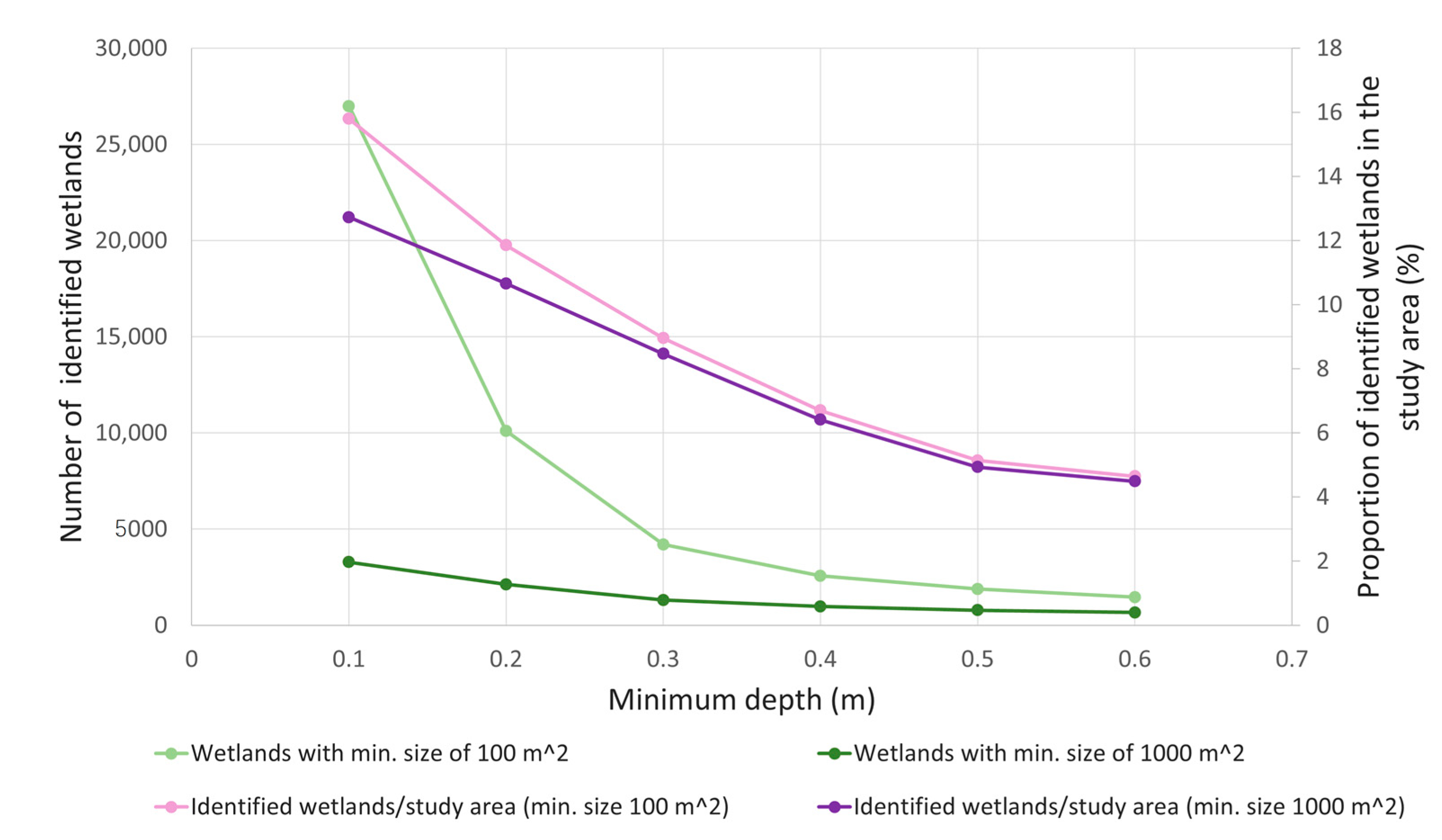
The number of wetlands detected by the model varied depending on the threshold values. When using small minimum wetland size (100 m2) and the shallowest minimum wetland depth (0.1 m), 27,000 wetlands were detected, covering 16% of the study area (Figure 5). When the threshold values were more constrained for both minimum wetland size (1000 m2) and depth (0.6 m), the number of wetlands detected decreased to around 700, covering around 4.5% of the study area (Figure 5). The number of detected wetlands did not vary greatly when changing the minimum depth from 0.3 to 0.6 m. Above a minimum wetland depth of 0.3 m, the proximity between the graphs representing the proportion and number of identified wetlands started to increase.
3.2. Similarity Analysis and Selection of Model Parameters
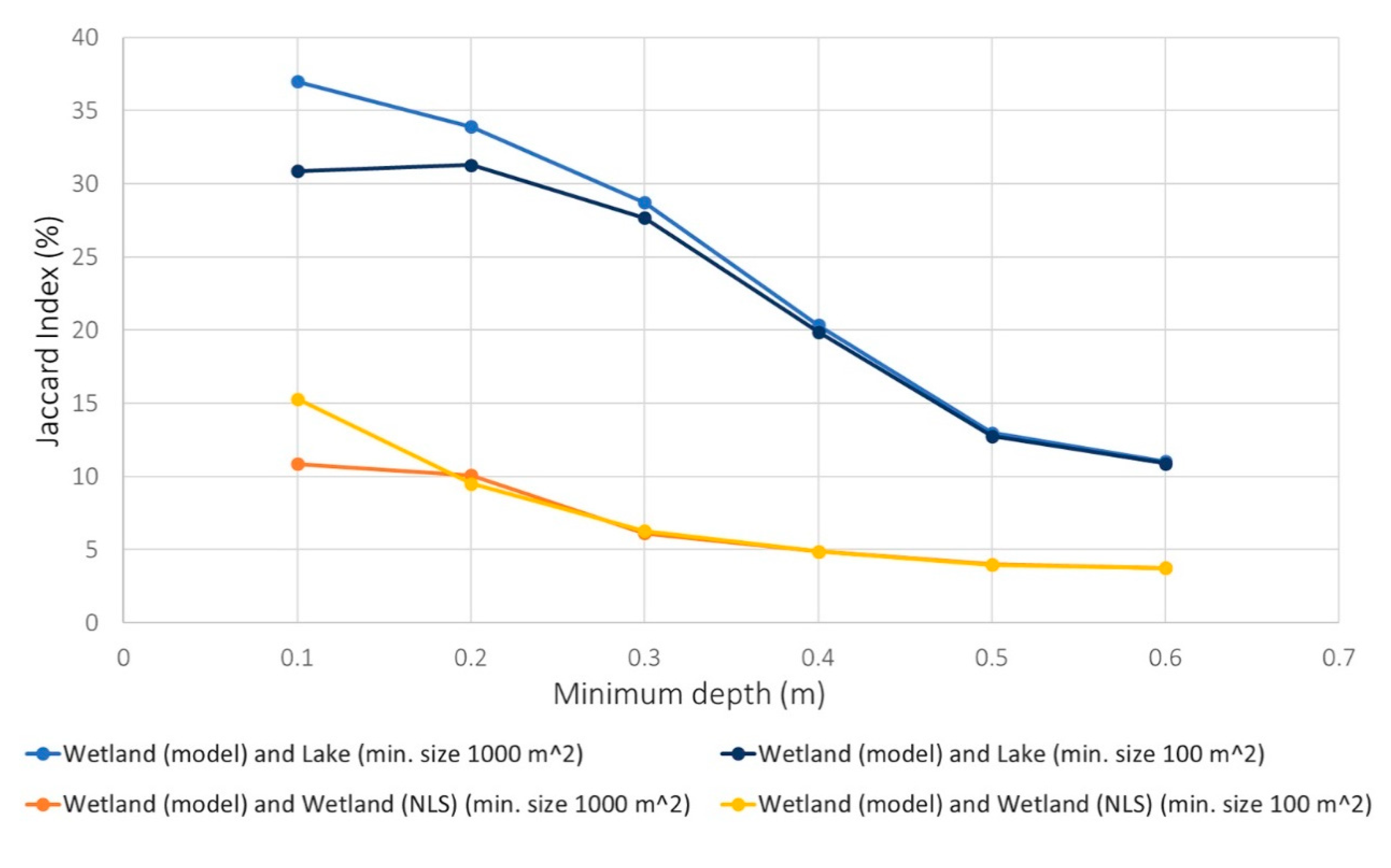
Wetlands identified by the model differed in spatial extent from the land cover map of wetlands from NLS Finland. Wetlands mapped by NLS Finland occupied 36% of the study area (Table 1) and coincided to 15% with the identified wetlands considering a minimum size of 100 m2 and depth of 0.1 m, and to around 11% with wetlands considering a minimum size of 1000 m2 and depth of 0.1 m (Figure 6). The lakes mapped by NLS Finland covered 8% of the study area (Table 1), and coincided to a greater extent with the identified wetlands, with almost 31% similarity when using threshold values of 100 m2 minimum size and 0.1 m depth, and 37% when using 1000 m2 minimum size and 0.1 m depth (Figure 6). When the minimum depth was ≤0.3 m, the similarity with lakes was higher for the minimum area of 1000 m2, while at minimum depths >0.3 m, the similarity with lakes was equally high for both minimum area thresholds. In general, similarities with both wetlands and lakes mapped by NLS Finland decreased when the minimum depth increased, except for minimum threshold values up to 0.2 m of minimum depth for wetlands and 0.3 m for lakes by NLS Finland.
Considering the vertical accuracy of the DEM (0.15–0.3 m) and the shallowness of a wetland with 0.1 m depth, it is not reliable to use this value as a minimum depth to detect potential wetlands. However, the vertical accuracy refers to absolute values, which indicates that within a small area, the relative vertical accuracy can be higher. Minimum depths ≥ 0.4 m did not affect the number of identified wetlands or significantly increase the similarity with the wetlands or lakes mapped by NLS Finland. A minimum depth of 0.2 m and 0.3 m showed relatively high similarity with both the NLS Finland wetlands and the lakes, although with slightly lower similarity for lakes. The difference in similarity when using 1000 m2 or 100 m2 was small, but a minimum wetland size of 1000 m2 showed higher similarity with the NLS Finland lakes and wetlands at a depth of 0.2 m. Based on these results, the thresholds of 0.2 m minimum depth and 1000 m2 minimum size were selected for further analyses of wetlands.
3.3. Mapping of Identified Wetlands
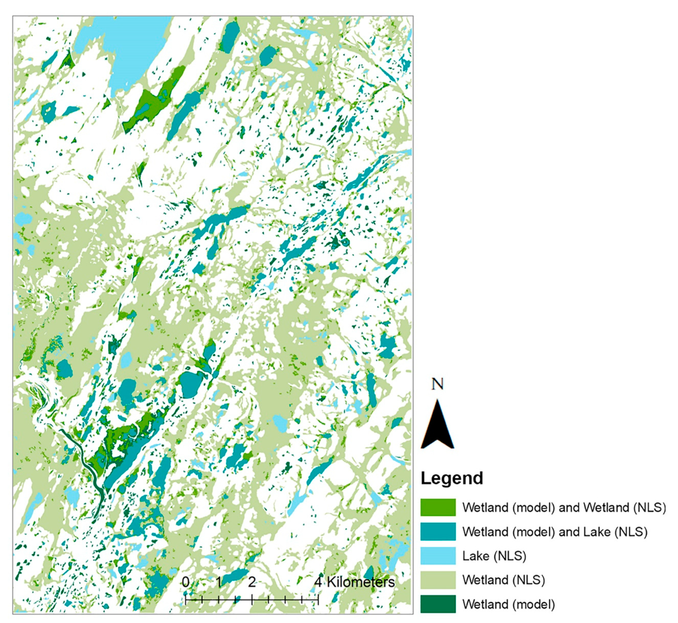
Overall, 2122 wetlands were identified in the study area by the model, covering an area of 23 km2. Areas where wetlands, lakes and rivers overlapped (11 km2) were not considered, resulting in total coverage of 12 km2 of wetlands (Table 2). Of these wetlands, 8 km2 corresponded to NLS Finland wetlands (64% user accuracy), while 69 km2 of the wetlands were missed (10% producer accuracy) (Table 2), with the F1 score for the wetland class being 17%. Figure 7 shows the cover of identified wetlands and their overlap with the wetlands and lakes mapped by NLS Finland.
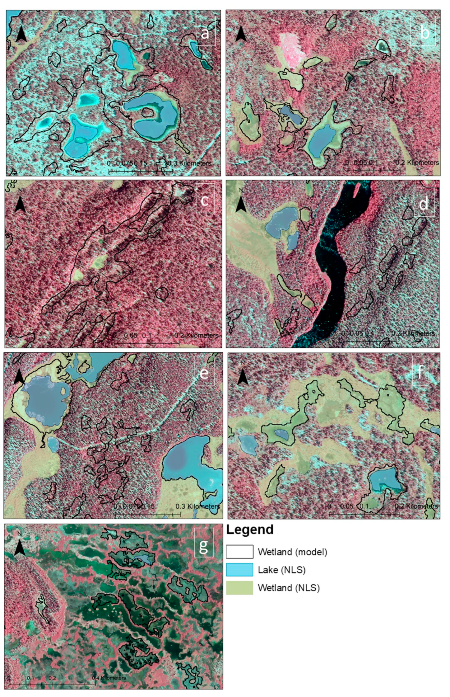
Figure 8 presents selected parts of the study area to illustrate the delineated potential wetlands on a smaller scale, with more details. On one hand, the methodology developed identified some potential wetland areas not mapped by NLS Finland. In Figure 8a, the terrain around lakes/ponds identified as wetland by the model, but not classified as wetland by NLS Finland, was partly peatland and partly upland forest, according to visual interpretation of the aerial image. In addition, four lakes/ponds observed in the aerial image to be inundated area (Figure 8a) were not identified by the NLS Finland mapping (as a lake or wetland), but they were correctly identified by the model. Figure 8b shows three small ponds that can give rise to wetlands, which were identified by the methodology, but left out of the NLS Finland map. Figure 8c shows an example of how the model sometimes covered larger areas than other mapping methods. In this example, the small patches of wetlands (NLS Finland) located at the bottom of the identified wetlands might be larger, according to visual interpretation of the aerial image. For example, the small pond located just above the wetland patches was not identified by NLS Finland, indicating that its mapping methodology missed some wetland areas. On the other hand, in some cases, the model failed to identify wetlands. Figure 8d,e show potential wetlands identified by the model that seem to be upland forest in visual interpretation of the aerial image. In addition, NLS Finland wetlands were not identified in the area. Figure 8f shows a situation where the identified wetlands coincided with wetlands by NLS Finland, but missed relatively large parts of the surrounding area, whereas the wetlands mapped by NLS Finland covered larger coherent areas of wetland. Figure 8g illustrates how the methodology sometimes had difficulty in mapping the wetland area, by identifying several patches spread within the study area. The wetlands by NLS Finland, which are not included in the images to enable the terrain below to be seen, provided coherent cover of the whole area.
3.4. Wetlandscape Connectivity
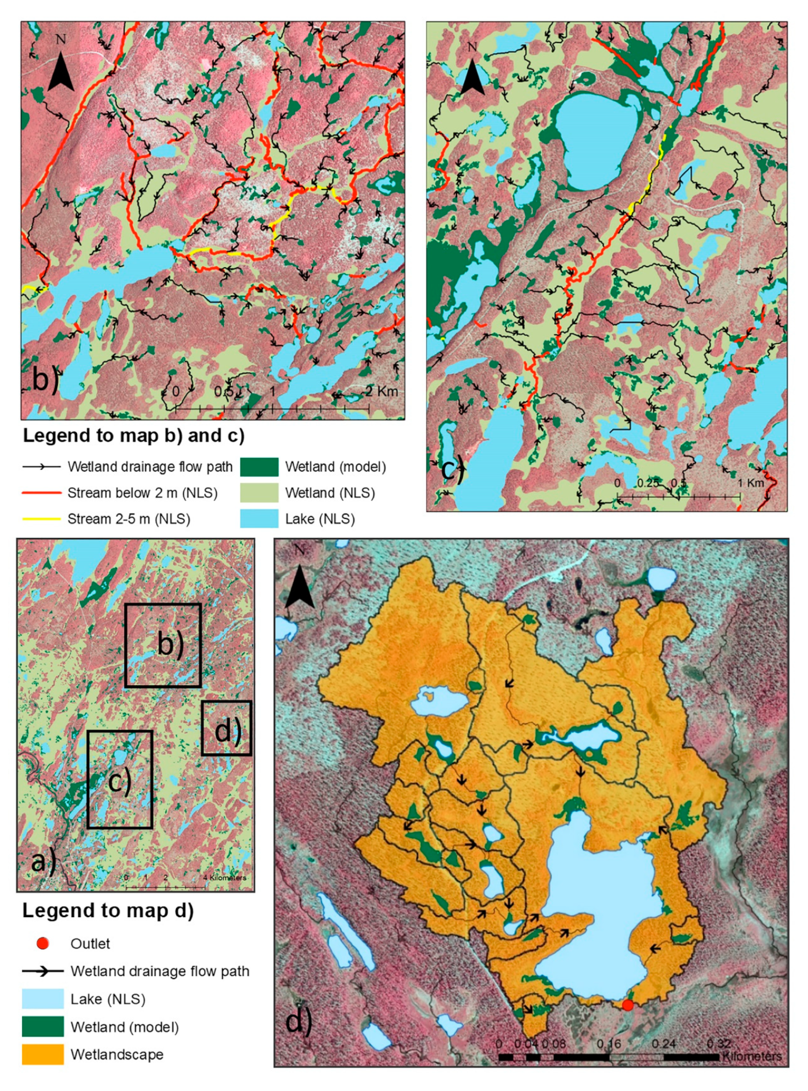
Figure 9 shows the results obtained from the connectivity analysis, illustrated for some selected areas (shown in Figure 9a). Figure 9b,c show the connectivity among wetlands in selected parts of the study area, where the modelled drainage flow paths from the identified wetland are delineated together with stream waters and wetlands mapped by NLS Finland. Figure 9d shows an example of a wetlandscape identified in the study area, illustrating how water in the landscape flows from upstream wetlands towards a larger identified wetland area, which surrounds a lake, through other identified wetlands and lakes located along its way. Water discharges at the outlet in the southernmost part of the lake. The yellow/orange area in Figure 9d is the spatial extent of the wetlandscape, which is made up of watersheds from each identified wetland forming a sub-catchment in the study area. The areas surrounding the delineated wetlandscape do not have a direct connection to the wetlands within the wetlandscape or to the outlet. In general, according to the flow path results, almost 60% of the identified wetlands in the study area were shown to receive water from no other wetland, comprising isolated wetlands. Around 23% received water from one other upstream wetland, while 16% of the identified wetlands received water from two to eight other upstream wetlands. The remaining 1% of identified wetlands received water from nine to 42 other upstream wetlands. The delineated flow paths extended over 410 km, of which 250 km were on NLS Finland wetlands, representing almost 61% of the delineated flow paths. Approximately 11% of the stream water mapped by NLS Finland was similar to the delineated flow paths.
4. Discussion
4.1. Model Performance in Identification of Wetlands
The methodology developed allowed the partial identification of wetlands and their interconnectivity. Of the wetlands identified using model threshold values of 1000 m2 for minimum size and 0.2 m for minimum depth, 64% were also mapped as wetlands by NLS Finland. According to visual interpretation of the aerial image, the remaining 36% of identified wetlands comprised actual wetland areas not mapped by NLS Finland and areas incorrectly classified as wetlands by the model. However, only 10% of the wetlands by NLS were identified, and the F1 score was only 17%, indicating that the methodology did not cover the full extent of wetlands in the area. Nevertheless, earlier studies have shown that topographic maps such as the used NLS topographic database have uncertainties and have misclassified wetland areas [37]; therefore, the accuracy assessment results have uncertainties and should be treated critically.
Due to low producer accuracy in particular, the methodology cannot be used alone to map peatland and wetland areas in northern landscapes. One reason for the low coverage and low producer accuracy obtained was likely to be the assumptions made when modelling the complex hydrology and characteristics of wetlands. The methodology only uses DEM and two parameters, minimum wetland size and depth, while other factors that can indicate wetland area are not considered. The wetlands in the study area mostly consist of aapa mires [62], i.e., hydrologically continuous areas alternating with flarks (hollows) and strings (intervening ridges) [63] (Figure 8g). Aapa mires are not necessarily located in depressions and some can even be located on slopes [64], maintained by good access to water. These types of wetlands are difficult to map by assuming that wetlands are located in depressions and by using only two parameters (size and depth). Therefore, these assumptions might affect the model’s accuracy in delineation of wetlands. Additionally, identification of wetlands in this study was based on the premise that surface depressions often give rise to temporary, seasonal or permanent wetlands, since runoff from upslope areas accumulates at downslope sites within the landscape. Thus, for study areas flatter than the site in this study, the method might have more difficulties in identifying wetlands. Furthermore, the study site is known to be a wetland-rich area, which increased the probability of actually identifying wetlands.
The approach used in this study for delineating potential wetlands using DEM was first developed by Wu and Lane [51] to detect actual wetland landscapes in the Pipestem river sub-basin in the prairie pothole region (PPR) of North Dakota. It is therefore not developed specifically to identify potential wetlands in a flat northern boreal landscape with a subarctic climate. However, there are some similarities between PPR and northern boreal landscapes, since PPR is characterised by small (median size 1600 m2) and shallow (generally less than 1 m) wetlands [51], while the wetlands identified in this study had a median size of 2200 m2 and a mean depth of 0.36 m.
The methodology can be used as a complement to other mapping methods, such as field work, aerial image interpretation, other DEM-based methods [36,37] or more automated remote sensing-based land cover classifications [34,35]. Moreover, since many of the existing topographic maps, such as the NLS Finland topographic database used as a source of reference data in this study, miss out wet areas, DEM-based methods can be used to improve the existing maps. In a study in Sweden, Lidberg et al. [37] used fieldwork data as training and validation data, and classified wetlands with the help of existing maps and topographic indices, including topographic wetness and depth to water. The inclusion of topographic indices increased the accuracy of mapping compared with existing maps, with overall accuracy increasing from 74% to 84% and producer accuracy increasing from 36% to 75%. High classification accuracies can also be obtained with different remote sensing datasets, in particular if different types of data are included in the classification task. In a study in northern Sweden, Karlson et al. [38] obtained classification accuracy of 91% when delineating peatlands with Sentinel-1 synthetic aperture radar and LIDAR DEM data. In some other studies, moderate to high producers’ and total classification accuracies (>60%) have been obtained in wetland delineation and boreal wetland land cover classifications with different remote sensing datasets, such as optical, LIDAR and synthetic aperture radar data [36,65,66]. Accuracies can be much lower, even <20%, in wetland identification when using only a single data source [66], which shows that multiple data sources should be used in wetland delineation, including DEM, optical and synthetic aperture radar data. Most of the remote sensing-based wetland mappings require training data that can be collected through field work or an existing map of wetlands. However, some DEM-based approaches, such as topographic indices and the method developed in this study, do not necessarily require training data, which is definitely a strength of DEM-based methods. The method may be improved by combining it with other methods, such as the topographic wetness (besides using additional data). Future studies should test how the depression-based DEM method used in this study compares with other DEM and remote sensing-based methods in different landscapes, and how well it can complement other mapping and datasets. It is also suggested to combine DEM and other data to improve the method of mapping wetlands.
While the threshold values set may limit the identification of wetlands, the inclusion of additional factors that can indicate wetland, such as soil type, soil moisture, vegetation type and groundwater exchange, can relatively easily increase the potential of the methodology. In future research, the focus should be on developing the methodology in that regard. An advantage of the methodology is the use of DEM data, which are usually available. A number of countries collect high-resolution DEM, while more global high-resolution datasets such as the ArcticDEM [67] are also freely accessible to different practitioners, and thus can be used to identify wetlands. The use of only two parameters (minimum wetland size and depth) makes the method simple and, according to the results, enables it to identify wetlands in areas where other methods do not, specifically areas around lakes and ponds. Field work could be targeted at these areas to validate the findings.
Despite the regional importance of Arctic wetlands, the datasets currently available (e.g., those reported by Arino et al. [68]; Chen et al. [69]; Kobayashi et al. [70]; Lehner and Döll [71]; Schroeder et al. [72] do not have enough accuracy and full coverage of the Arctic region. Due to substantial differences between wetlands, finding a standard method to outline all wetlands can be challenging, although there are several indicators available to define location of potential wetlands. Such indicators include different type of vegetation, hydrology, soil type, proximity to water, and landform [73] that should be delineated from multiple different data sources. Several databases, including national, regional, and global, to some extent can define wetland areas, but most available databases don’t have sufficient resolution to accurately identify future vulnerable wetland areas. Moreover, none of the high-resolution datasets e.g., for soil type and soil moisture covers the entire Arctic region, indicating a need to consider several datasets.
The methodology developed in this study can also be used to increase understanding of wetland dynamics. For example, results could be regenerated using different DEMs collected at different times, such as multiple times during a year or from multiple years, and comparing these. Such analysis could show how the landscape and thereby the connectivity between wetlands changes, e.g., which flow paths are transient and which are more permanent. Furthermore, in flat landscapes such as the study area used in this research, catchment boundaries are not necessarily stable over time and water from a particular wetland might flow to different catchments, depending on the temporal dynamics.
4.2. Hydrological Connectivity of Wetlands and Wetland Management
Regarding the results from the connectivity analysis, delineation of the wetlandscape was relatively straightforward once the wetlands were identified and their catchments and drainage flow paths were delineated. Furthermore, the delineated flow paths indicated in many cases flow directions from the identified wetlands towards lakes or stream waters. These flow paths were only partly similar (11%) to streams mapped by NLS Finland, but were largely (61%) located in wetlands mapped by NLS Finland. This suggests that water flows and also spreads along the mapped flow paths. Hence, even if the identified wetlands do not cover all wetlands, the identified wetlands together with their delineated drainage flow paths define a more coherent spread of wetlands. However, it has to be considered that the delineation of the wetlandscape is carried out with the help of topographical data only and is based on the identified wetlands. The methodology has managed to delineate a wetlandscape in practice from a conceptual idea suggested by Thorslund et al. [38]. Further investigations regarding the mapped wetlandscapes and their specific characteristics were not conducted in this study. In future studies, the connectivity analysis could be extended by connecting the findings to data obtained with techniques such as dye tracers [39]. Moreover, the connectivity analysis could include groundwater fluctuations by monitoring the groundwater levels with pressure transducers [42].
Modelling hydrological connectivity is important, since it acts as the mechanism by which physical, biological and chemical materials are transported and distributed in the landscape [26,74]. These elements are crucial for the ecosystems that exist in and around wetlands, contributing more than 20% of the total value of ecosystem services globally [75]. These ecosystem services have the ability e.g., to sequester carbon, protect water quality, regulate flooding, support biodiversity and, not least, manage climate change. Understanding connectivity is a way to understand interactions between freshwater systems and prepare to meet current and future challenges, as has been especially emphasised in recent studies [2,38,76,77,78]. The ability of the method to delineate wetlandscapes based on connectivity allows the total hydrological catchment of multiple wetlands to be analysed. The method could thus be used for tracking flows of water through a wetlandscape and identifying those that are more vulnerable and need more protection, e.g., flows that are more or less sensitive to changes as a result of climate change, land use or water use. Application of the method to compare DEMs acquired at different times could also be used to easily assess wetland connectivity over time, which will vary with climate change. In this way, the method can be used for remote monitoring of climate impacts on wetland connectivity. Another area of application where the method could be used is the poorly studied land-to-water (lateral) transport of carbon, which affects ecosystems and the biochemistry of freshwater [79]. Wetlands receive large amounts of carbon from the terrestrial environment and play a major role in transporting, transforming, storing and filtering water, sediments and solutes [80,81]. This functioning will be affected by climate-induced changes in the hydrological cycle [82,83], thereby altering the carbon cycle. The ability to map the connectivity between wetlands could be useful in research to quantify future transport of carbon and the carbon balance of watersheds.
5. Conclusions
In this research, DEM data were used to inventory wetlands in northern landscapes, and a depression-based method was used to apply the conceptual wetlandscape concept to wetland connectivity analysis. However, the wetlands identified in the study area did not cover the full extent of wetlands based on existing wetland maps. Thus the method cannot be used alone to map peatland and wetland areas in northern landscapes, and should be complemented with other datasets and mapping methods, such as field work and remote sensing-based mappings. Importantly, the delineated wetlandscapes achieved with the depression-based DEM method improved understanding of the hydrologically coupled system of several wetlands and their connectivity. Future research is required to improve the method, which could benefit from including more data, such as soil moisture and vegetation, and from validating the findings through field studies given the uncertainties associated with current NLS Finland map of wetlands. In the present application, the method was used to map wetlands and their hydrological connectivity, which is fundamental and valuable information for the management and protection of northern wetland landscapes.
Author Contributions
Z.K. initiated the research and planned it together with E.S. and A.R. E.S. conducted the data analyses under supervision by Z.K. and A.R. E.S. wrote the first draft of the manuscript and finalised it together with Z.K., C.S.S.F. and A.R. All authors have read and agreed to the published version of the manuscript.
Funding
This research was funded by Arctic Avenue and ASIAQ mobility grants from Stockholm University.
Acknowledgments
We acknowledge Master thesis research performed by E.S., which laid the foundation for this article.
Conflicts of Interest
The authors declare no conflict of interest. The funders had no role in the design of the study; in the collection, analyses, or interpretation of data; in the writing of the manuscript, or in the decision to publish the results.
References
- Ramsar Focuses on Arctic Wetlands|Ramsar. Available online: https://www.Ramsar.org/news/ramsar-focuses-on-arctic-wetlands (accessed on 12 July 2020).
- Destouni, G.; Jaramillo, F.; Prieto, C. Hydroclimatic shifts driven by human water use for food and energy production. Nat. Clim. Chang. 2013, 3, 213–217. [Google Scholar] [CrossRef]
- Seneviratne, S.I.; Lüthi, D.; Litschi, M.; Schär, C. Land–atmosphere coupling and climate change in Europe. Nat. Cell Biol. 2006, 443, 205–209. [Google Scholar] [CrossRef] [PubMed]
- Wetlands: Source of Sustainable Livelihoods. Available online: https://www.ramsar.org/sites/default/files/fs_7_livelihoods_en_v5_2.pdf (accessed on 20 July 2020).
- Quin, A.; Destouni, G. Large-scale comparison of flow-variability dampening by lakes and wetlands in the landscape. Land Degrad. Dev. 2018, 29, 3617–3627. [Google Scholar] [CrossRef] [Green Version]
- Golden, H.E.; Creed, I.F.; Ali, G.; Basu, N.B.; Neff, B.P.; Rains, M.C.; McLaughlin, D.L.; Alexander, L.C.; Ameli, A.A.; Christensen, J.R.; et al. Integrating geographically isolated wetlands into land management decisions. Front. Ecol. Environ. 2017, 15, 319–327. [Google Scholar] [CrossRef]
- Creed, I.F. Groundwaters at Risk: Wetland Loss Changes Sources, Lengthens Pathways, and Decelerates Rejuvenation of Groundwater Resources. JAWRA J. Am. Water Resour. Assoc. 2019, 55, 294–306. [Google Scholar] [CrossRef]
- Verhoeven, J.T.A.; Arheimer, B.; Yin, C.; Hefting, M.M. Regional and global concerns over wetlands and water quality. Trends Ecol. Evol. 2006, 21, 96–103. [Google Scholar] [CrossRef]
- Gibbs, J.P. Wetland Loss and Biodiversity Conservation. Conserv. Biol. 2000, 14, 314–317. [Google Scholar] [CrossRef] [Green Version]
- Mitsch, W.J.; Bernal, B.; Nahlik, A.M.; Mander, Ü.; Zhang, L.; Anderson, C.J.; Jorgensen, S.E.; Brix, H. Wetlands, carbon, and climate change. Landsc. Ecol. 2013, 28, 583–597. [Google Scholar] [CrossRef]
- Karlsson, J.M.; Bring, A.; Peterson, G.D.; Gordon, L.J.; Destouni, G. Opportunities and limitations to detect climate-related regime shifts in inland Arctic ecosystems through eco-hydrological monitoring. Environ. Res. Lett. 2011, 6. [Google Scholar] [CrossRef]
- Lindwall, F.; Svendsen, S.S.; Nielsen, C.S.; Michelsen, A.; Rinnan, R. Warming increases isoprene emissions from an arctic fen. Sci. Total. Environ. 2016, 553, 297–304. [Google Scholar] [CrossRef]
- Morison, M.Q.; Macrae, M.L.; Petrone, R.M.; Fishback, L. Seasonal dynamics in shallow freshwater pond-peatland hydrochemical interactions in a subarctic permafrost environment. Hydrol. Process. 2017, 31, 462–475. [Google Scholar] [CrossRef]
- Pavón-Jordán, D.; Santangeli, A.; Lehikoinen, A. Effects of flyway-wide weather conditions and breeding habitat on the breeding abundance of migratory boreal waterbirds. J. Avian Biol. 2017, 48, 988–996. Available online: https://researchportal.helsinki.fi/en/publications/effects-of-flyway-wide-weather-conditions-and-breeding-habitat-on (accessed on 20 July 2020). [CrossRef] [Green Version]
- Van Der Kolk, H.-J.; Heijmans, M.M.P.D.; Van Huissteden, K.; Pullens, J.W.M.; Berendse, F. Potential Arctic tundra vegetation shifts in response to changing temperature, precipitation and permafrost thaw. Biogeosciences 2016, 13, 6229–6245. [Google Scholar] [CrossRef] [Green Version]
- Keesstra, S.; Nunes, J.P.; Novara, A.; Finger, D.; Avelar, D.; Kalantari, Z.; Cerdà, A. The superior effect of nature based solutions in land management for enhancing ecosystem services. Sci. Total. Environ. 2018, 997–1009. [Google Scholar] [CrossRef] [Green Version]
- Cohen-Shacham, E.; Walters, G.; Janzen, C.; Maginnis, S. Nature-Based Solutions to Address Global Societal Challenges; IUCN: Gland, Switzerland, 2016; 97p. [Google Scholar]
- Stocker, T.F.; Qin, D.; Plattner, G.-K.; Tignor, M.; Allen, S.K.; Boschung, J.; Nauels, A.; Xia, Y.; Bex, V.; Midgley, P.M. Climate Change 2013: The physical Science Basis; Working Group I Contribution to the Fifth Assessment Report of the Intergovernmental Panel on Climate Change; Cambridge University Press: Cambridge, UK, 2013; Available online: https://boris.unibe.ch/71452/ (accessed on 20 July 2020). [CrossRef] [Green Version]
- Erwin, K.L. Wetlands and global climate change: The role of wetland restoration in a changing world. Wetl. Ecol. Manag. 2009, 17, 71–84. [Google Scholar] [CrossRef]
- Box, J.; Colgan, W.T.; Christensen, T.R.; Schmidt, N.M.; Lund, M.; Parmentier, F.-J.W.; Brown, R.; Bhatt, U.S.; Euskirchen, E.S.; Romanovsky, V.E.; et al. Key indicators of Arctic climate change: 1971–2017. Environ. Res. Lett. 2019, 14, 045010. [Google Scholar] [CrossRef]
- Serreze, M.C.; Walsh, J.E.; Iii, F.S.C.; Osterkamp, T.; Dyurgerov, M.; Romanovsky, V.; Oechel, W.C.; Morison, J.; Zhang, T.; Barry, R.G. Observational Evidence of Recent Change in the Northern High-Latitude Environment. Clim. Chang. 2000, 46, 159–207. [Google Scholar] [CrossRef]
- Land, M.; Carson, M. Sustainable Management and Resilience of Arctic Wetlands—Scoping Study. Available online: https://www.sei.org/publications/sustainable-management-resilience-arctic-wetlands/ (accessed on 12 July 2020).
- Juvonen, S.-K.; Kurikka, T. Finland’s Ramsar Wetlands Action Plan 2016–2020|InforMEA. Available online: https://www.informea.org/en/finland%E2%80%99s-ramsar-wetlands-action-plan-2016%E2%80%932020 (accessed on 26 July 2020).
- Hu, S.; Niu, Z.; Chen, Y.; Li, L.; Zhang, H. Global wetlands: Potential distribution, wetland loss, and status. Sci. Total. Environ. 2017, 586, 319–327. [Google Scholar] [CrossRef]
- Gunnarsson, U.; Löfroth, M. Våtmarksinventeringen: Resultat Från 25 Års Inventeringar: Nationell Slutrapport för Våtmarksinventeringen (VMI) i Sverige. Naturvårdsverket. 2009. Available online: http://urn.kb.se/resolve?urn=urn:nbn:se:uu:diva-120460 (accessed on 10 August 2020).
- Leibowitz, S.G.; Mushet, D.M.; Newton, W.E. Intermittent Surface Water Connectivity: Fill and Spill Vs. Fill and Merge Dynamics. Wetlands 2016, 36, 323–342. [Google Scholar] [CrossRef]
- Freeman, M.C.; Pringle, C.M.; Jackson, C.R. Hydrologic Connectivity and the Contribution of Stream Headwaters to Ecological Integrity at Regional Scales. JAWRA J. Am. Water Resour. Assoc. 2007, 43, 5–14. [Google Scholar] [CrossRef]
- Li, T.; Raivonen, M.; Alekseychik, P.; Aurela, M.; Lohila, A.; Zheng, X.; Zhang, Q.; Wang, G.; Mammarella, I.; Rinne, J.; et al. Importance of vegetation classes in modeling CH4 emissions from boreal and subarctic wetlands in Finland. Sci. Total. Environ. 2016, 572, 1111–1122. [Google Scholar] [CrossRef] [PubMed]
- Craft, C. Creating and Restoring Wetlands: From Theory to Practice; Elsevier: Amsterdam, The Netherlands, 2015; 360p. [Google Scholar]
- Swindles, G.T.; Morris, P.J.; Mullan, D.J.; Payne, R.J.; Roland, T.P.; Amesbury, M.J.; Lamentowicz, M.; Turner, T.E.; Gallego-Sala, A.; Sim, T.; et al. Widespread drying of European peatlands in recent centuries. Nat. Geosci. 2019, 12, 922–928. [Google Scholar] [CrossRef]
- Hugelius, G.; Loisel, J.; Chadburn, S.; Jackson, R.B.; Jones, M.; Macdonald, G.; Marushchak, M.; Olefeldt, D.; Packalen, M.; Siewert, M.B.; et al. Large stocks of peatland carbon and nitrogen are vulnerable to permafrost thaw. Proc. Natl. Acad. Sci. USA 2020, 117, 20438–20446. [Google Scholar] [CrossRef] [PubMed]
- Golden, H.E.; Lane, C.R.; Amatya, D.M.; Bandilla, K.W.; Kiperwas, H.R.; Knightes, C.D.; Ssegane, H. Hydrologic connectivity between geographically isolated wetlands and surface water systems: A review of select modeling methods. Environ. Model. Softw. 2014, 53, 190–206. [Google Scholar] [CrossRef]
- Ghajarnia, N.; Destouni, G.; Thorslund, J.; Kalantari, Z.; Åhlén, I.; Anaya-Acevedo, J.A.; Blanco-Libreros, J.F.; Borja, S.; Chalov, S.; Chalova, A.; et al. Data for wetlandscapes and their changes around the world. Earth Syst. Sci. Data 2020, 12, 1083–1100. [Google Scholar] [CrossRef]
- Bourgeau-Chavez, L.; Endres, S.; Powell, R.; Battaglia, M.; Benscoter, B.; Turetsky, M.; Kasischke, E.; Banda, E. Mapping boreal peatland ecosystem types from multitemporal radar and optical satellite imagery. Can. J. For. Res. 2017, 47, 545–559. [Google Scholar] [CrossRef]
- Karlson, M.; Gålfalk, M.; Crill, P.; Bousquet, P.; Saunois, M.; Bastviken, D. Delineating northern peatlands using Sentinel-1 time series and terrain indices from local and regional digital elevation models. Remote. Sens. Environ. 2019, 231, 111252. [Google Scholar] [CrossRef]
- Murphy, P.N.C.; Ogilvie, J.; Connor, K.; Arp, P.A. Mapping wetlands: A comparison of two different approaches for New Brunswick, Canada. Wetlands 2007, 27, 846–854. [Google Scholar] [CrossRef]
- Lidberg, W.; Nilsson, M.; Ågren, A.M. Using machine learning to generate high-resolution wet area maps for planning forest management: A study in a boreal forest landscape. Ambio 2020, 49, 475–486. [Google Scholar] [CrossRef] [Green Version]
- Thorslund, J.; Jarsjo, J.; Jaramillo, F.; Jawitz, J.W.; Manzoni, S.; Basu, N.B.; Chalov, S.R.; Cohen, M.J.; Creed, I.F.; Goldenberg, R.; et al. Wetlands as large-scale nature-based solutions: Status and challenges for research, engineering and management. Ecol. Eng. 2017, 108, 489–497. [Google Scholar] [CrossRef]
- Dai, L.; Zhang, Y.; Liu, Y.; Xie, L.; Zhao, S.; Zhang, Z.; Lv, X. Assessing hydrological connectivity of wetlands by dye-tracing experiment. Ecol. Indic. 2020, 119, 106840. [Google Scholar] [CrossRef]
- Mooney, S.J.; Morris, C. A morphological approach to understanding preferential flow using image analysis with dye tracers and X-ray Computed Tomography. Catena 2008, 73, 204–211. [Google Scholar] [CrossRef]
- Jones, E.H.; Smith, C.C. Non-equilibrium partitioning tracer transport in porous media: 2-D physical modelling and imaging using a partitioning fluorescent dye. Water Res. 2005, 39, 5099–5111. [Google Scholar] [CrossRef] [PubMed]
- Ferlatte, M.; Quillet, A.; Larocque, M.; Cloutier, V.; Pellerin, S.; Paniconi, C. Aquifer-peatland connectivity in southern Quebec (Canada). Hydrol. Process. 2015, 29, 2600–2612. [Google Scholar] [CrossRef] [Green Version]
- Allen, C.; Gonzales, R.; Parrott, L. Modelling the contribution of ephemeral wetlands to landscape connectivity. Ecol. Model. 2020, 419, 108944. [Google Scholar] [CrossRef]
- Winter, T.C.; Woo, M.-K. Hydrology of lakes and wetlands. In Surface Water Hydrology; Geological Society of America: Boulder, CO, USA, 1990; pp. 159–187. Available online: https://pubs.geoscienceworld.org/books/book/861/chapter/3920383/ (accessed on 22 July 2020).
- Woo, M.-K.; Young, K.L. High Arctic wetlands: Their occurrence, hydrological characteristics and sustainability. J. Hydrol. 2006, 320, 432–450. [Google Scholar] [CrossRef]
- Wu, Q.; Liu, H.; Wang, S.; Yu, B.; Beck, R.; Hinkel, K. A localized contour tree method for deriving geometric and topological properties of complex surface depressions based on high-resolution topographical data. Int. J. Geogr. Inf. Sci. 2015, 29, 2041–2060. [Google Scholar] [CrossRef]
- Peel, M.C.; Finlayson, B.L.; Mcmahon, T.A. Updated world map of the Köppen-Geiger climate classification. Hydrol. Earth Syst. Sci. Discuss. 2007, 4, 439–473. [Google Scholar] [CrossRef] [Green Version]
- FMI (Finnish Meteorological Institute). GHG Measurement Sites—Finnish Meteorological Institute. Kaamanen. Available online: https://en.ilmatieteenlaitos.fi/ghg-measurement-sites (accessed on 22 July 2020).
- Finnish Environment Institute (SYKE). Downloadable Spatial Datasets—Syke.fi. Available online: https://www.syke.fi/en-US/Open_information/Spatial_datasets/Downloadable_spatial_dataset#C (accessed on 7 September 2020).
- Fisher, P.F.; Tate, N.J. Causes and consequences of error in digital elevation models. Prog. Phys. Geogr. Earth Environ. 2006, 30, 467–489. [Google Scholar] [CrossRef]
- Wu, Q.; Lane, C.R. Delineating wetland catchments and modeling hydrologic connectivity using lidar data and aerial imagery. Hydrol. Earth Syst. Sci. 2017, 21, 3579–3595. [Google Scholar] [CrossRef] [Green Version]
- Wang, L.; Liu, H. An efficient method for identifying and filling surface depressions in digital elevation models for hydrologic analysis and modelling. Int. J. Geogr. Inf. Sci. 2006, 20, 193–213. [Google Scholar] [CrossRef]
- Region Group—Help|ArcGIS for Desktop. Available online: https://desktop.arcgis.com/en/arcmap/10.3/tools/spatial-analyst-toolbox/region-group.htm (accessed on 22 July 2020).
- Zonal Statistics—Help|ArcGIS for Desktop. Available online: https://desktop.arcgis.com/en/arcmap/10.3/tools/spatial-analyst-toolbox/zonal-statistics.htm (accessed on 22 July 2020).
- Flow Direction—Help|ArcGIS for Desktop. Available online: https://desktop.arcgis.com/en/arcmap/10.3/tools/spatial-analyst-toolbox/flow-direction.htm (accessed on 22 July 2020).
- O’Callaghan, J.F.; Mark, D.M. The extraction of drainage networks from digital elevation data. Comput. Vis Graph Image Process. 1984, 28, 323–344. [Google Scholar] [CrossRef]
- Flow Accumulation—Help|ArcGIS for Desktop. Available online: https://desktop.arcgis.com/en/arcmap/10.3/tools/spatial-analyst-toolbox/flow-accumulation.htm (accessed on 22 July 2020).
- Cost Path—Help|Documentation. Available online: https://pro.arcgis.com/en/pro-app/tool-reference/spatial-analyst/cost-path.htm (accessed on 22 July 2020).
- Geodata Portal Paikkatietoikkuna|National Land Survey of Finland. Available online: https://www.maanmittauslaitos.fi/en/e-services/geodata-portal-paikkatietoikkuna (accessed on 26 July 2020).
- Jaccard, P. The Distribution of the Flora in the Alpine Zone. New Phytol. 1912, 11, 37–50. [Google Scholar] [CrossRef]
- Chu, X.; Yang, J.; Chi, Y.; Zhang, J. Dynamic puddle delineation and modeling of puddle-to-puddle filling-spilling-merging-splitting overland flow processes. Water Resour. Res. 2013, 49, 3825–3829. [Google Scholar] [CrossRef]
- Aurela, M.; Laurila, T.; Tuovinen, J.-P. The timing of snow melt controls the annual CO2 balance in a subarctic fen. Geophys. Res. Lett. 2004, 31. Available online: https://agupubs.onlinelibrary.wiley.com/doi/abs/ (accessed on 22 July 2020). [CrossRef]
- Aapamyrar. Environmental Protection Agency Sweden. 2011. Available online: http://www.naturvardsverket.se/upload/stod-i-miljoarbetet/vagledning/natura-2000/naturtyper/myrar/vl-7310-aapamyr.pdf (accessed on 22 July 2020).
- Laitinen, J.; Rehell, S.; Huttunen, A.; Tahvanainen, T.; Heikkilä, R.; Lindholm, T. Mire systems in Finland—special view to aapa mires and their water-flow pattern. Suo 2007, 58, 1–26. [Google Scholar]
- Amani, M.; Salehi, B.; Mahdavi, S.; Granger, J.; Brisco, B. Wetland classification in Newfoundland and Labrador using multi-source SAR and optical data integration. GIScience Remote. Sens. 2017, 54, 779–796. [Google Scholar] [CrossRef]
- Merchant, M.A.; Warren, R.K.; Edwards, R.; Kenyon, J.K. An Object-Based Assessment of Multi-Wavelength SAR, Optical Imagery and Topographical Datasets for Operational Wetland Mapping in Boreal Yukon, Canada. Can. J. Remote. Sens. 2019, 45, 308–332. [Google Scholar] [CrossRef]
- Porter, C.; Morin, P.; Howat, I.; Noh, M.J.; Bates, B.; Peterman, K.; Keesey, S.; Schlenk, M.; Gardiner, J.; Tomko, K. ArcticDEM. Harvard Dataverse. 2018. Available online: https://dataverse.harvard.edu/dataset.xhtml?persistentId=doi:10.7910/DVN/OHHUKH (accessed on 16 September 2020).
- Arino, O.; Ramos Perez, J.J.; Kalogirou, V.; Bontemps, S.; Defourny, P.; Van Bogaert, E. Global Land Cover Map for 2009 (GlobCover 2009). ©European Space Agency (ESA) & Université Catholique de Louvain (UCL). PANGAEA, 2012. Available online: https://doi.pangaea.de/10.1594/PANGAEA.787668 (accessed on 30 October 2020).
- Chen, J.; Chen, J.; Liao, A.; Cao, X.; Chen, L.; Chen, X.; He, C.; Han, G.; Peng, S.; Lu, M.; et al. Global land cover mapping at 30m resolution: A POK-based operational approach. ISPRS J. Photogramm. Remote. Sens. 2015, 103, 7–27. [Google Scholar] [CrossRef] [Green Version]
- Tateishi, R.; Uriyangqai, B.; Al-Bilbisi, H.; Ghar, M.A.; Tsend-Ayush, J.; Kobayashi, T.; Kasimu, A.; Hoan, N.T.; Shalaby, A.; Alsaaideh, B.; et al. Production of Global Land Cover Data—GLCNMOJ. Geogr Geol. 2017, 9, 1. [Google Scholar]
- Lehner, B.; Döll, P. Development and validation of a global database of lakes, reservoirs and wetlands. J. Hydrol. 2004, 296, 1–22. [Google Scholar] [CrossRef]
- Schroeder, R.; McDonald, K.C.; Chapman, B.; Jensen, K.; Podest, E.; Tessler, Z.D.; Bohn, T.J.; Zimmermann, R. Development and Evaluation of a Multi-Year Fractional Surface Water Data Set Derived from Active/Passive Microwave Remote Sensing Data. Remote. Sens. 2015, 7, 16688–16732. [Google Scholar] [CrossRef] [Green Version]
- Tiner, R. Ecology of Wetlands: Classification Systems. In Encyclopedia of Inland Waters; Elsevier BV: Amsterdam, The Netherlands, 2009; pp. 516–525. Available online: https://linkinghub.elsevier.com/retrieve/pii/B9780123706263000570 (accessed on 19 September 2020).
- Zamberletti, P.; Zaffaroni, M.; Accatino, F.; Creed, I.F.; De Michele, C. Connectivity among wetlands matters for vulnerable amphibian populations in wetlandscapes. Ecol. Model. 2018, 384, 119–127. [Google Scholar] [CrossRef]
- Braat, L.; De Groot, R.; Sutton, P.C.; Van Der Ploeg, S.; Anderson, S.J.; Kubiszewski, I.; Farber, S.; Turner, R.K. Changes in the global value of ecosystem services. Glob. Environ. Chang. 2014, 26, 152–158. [Google Scholar] [CrossRef]
- Seifollahi-Aghmiuni, S.; Nockrach, M.; Kalantari, Z. The Potential of Wetlands in Achieving the Sustainable Development Goals of the 2030 Agenda. Water 2019, 11, 609. [Google Scholar] [CrossRef] [Green Version]
- Cohen, M.J.; Creed, I.F.; Alexander, L.; Basu, N.B.; Calhoun, A.J.K.; Craft, C.; D’Amico, E.; DeKeyser, E.; Fowler, L.; Golden, H.E.; et al. Do geographically isolated wetlands influence landscape functions? Proc. Natl. Acad. Sci. USA 2016, 113, 1978–1986. [Google Scholar] [CrossRef] [Green Version]
- Thorsteinsson, T.; Pundsack, J. Arctic-HYDRA Consortium (2010). Arctic-HYDRA: The Arctic Hydrological Cycle Monitoring, Modelling and Assessment Programme. Arctic Hydra. 2010. Available online: http://arctichydra.arcticportal.org/ (accessed on 21 August 2020).
- Tank, S.E.; Fellman, J.B.; Hood, E.; Kritzberg, E.S. Beyond respiration: Controls on lateral carbon fluxes across the terrestrial-aquatic interface. Limnol. Oceanogr. Lett. 2018, 3, 76–88. [Google Scholar] [CrossRef]
- Ameli, A.A.; Creed, I.F. Quantifying hydrologic connectivity of wetlands to surface water systems. Hydrol. Earth Syst. Sci. 2017, 21, 1791–1808. [Google Scholar] [CrossRef] [Green Version]
- Groß, E.; Mård, J.; Kalantari, Z.; Bring, A. Links between Nordic and Arctic hydroclimate and vegetation changes: Contribution to possible landscape-scale nature-based solutions. Land Degrad. Dev. 2018, 29, 3663–3673. [Google Scholar] [CrossRef] [Green Version]
- Borja, S.; Kalantari, Z.; Destouni, G. Global Wetting by Seasonal Surface Water over the Last Decades. Earth’s Futur. 2020, 8. [Google Scholar] [CrossRef] [Green Version]
- Ghajarnia, N.; Kalantari, Z.; Orth, R.; Destouni, G. Close co-variation between soil moisture and runoff emerging from multi-catchment data across Europe. Sci. Rep. 2020, 10, 4817. [Google Scholar] [CrossRef] [PubMed]
Figure 1.
(a) Location of the Kaamanen study area in Finland, and (b) true-colour aerial image (National Land Survey of Finland) showing the extent of the site.
Figure 1.
(a) Location of the Kaamanen study area in Finland, and (b) true-colour aerial image (National Land Survey of Finland) showing the extent of the site.

Figure 2.
Flowchart of the processes executed to delineate depressions, wetland catchments and flow paths. The illustration shows the operators and the created operation outputs and how they are used.
Figure 2.
Flowchart of the processes executed to delineate depressions, wetland catchments and flow paths. The illustration shows the operators and the created operation outputs and how they are used.

Figure 3.
Venn diagram illustrating (a) the intersection and (b) the union of two datasets (A and B).
Figure 3.
Venn diagram illustrating (a) the intersection and (b) the union of two datasets (A and B).

Figure 4.
(a) Schematic representation of the wetland identification process and connectivity. When depression A fills (1), it starts to spill to downstream depression B (2). When depression B fills, it starts to spill to depression C. When C is filled it merges with B (3) and forms depression D. (b) Illustration of a wetlandscape, including different wetlands connected by drainage flow paths and sharing the same drainage outlet.

Figure 5.
Difference between number of wetlands identified by the model (pink/purple lines) and wetlands mapped by National Land Survey (NLS) Finland (green lines) at different minimum wetland area thresholds (100 m2 and 1000 m2) and minimum wetland depths.
Figure 5.
Difference between number of wetlands identified by the model (pink/purple lines) and wetlands mapped by National Land Survey (NLS) Finland (green lines) at different minimum wetland area thresholds (100 m2 and 1000 m2) and minimum wetland depths.

Figure 6.
Similarity according to the Jaccard index between the identified wetlands (model results) and wetlands and lakes mapped by NLS Finland, for different minimum depth and minimum wetland size thresholds.
Figure 6.
Similarity according to the Jaccard index between the identified wetlands (model results) and wetlands and lakes mapped by NLS Finland, for different minimum depth and minimum wetland size thresholds.

Figure 7.
Wetlands identified in the study area when using a minimum wetland depth of 0.2 m and minimum wetland size of 1000 m2 in modelling, and overlap with available maps of wetlands and lakes produced by NLS Finland.
Figure 7.
Wetlands identified in the study area when using a minimum wetland depth of 0.2 m and minimum wetland size of 1000 m2 in modelling, and overlap with available maps of wetlands and lakes produced by NLS Finland.

Figure 8.
Examples of sites within the study area showing identification of potential wetlands by the model using thresholds of 1000 m2 minimum size and 0.2 m depth, on top of false-colour aerial images (©National Land Survey of Finland). The site in (a) was covered by NLS Finland wetlands, but the relevant colour coding is omitted to reveal the terrain below.

Figure 9.
(a) Map showing location of the sites shown in (b–d) in the study area. (b,c) Areas with the identified wetlands and their drainage flow path, together with existing streams mapped by NLS Finland. (d) Wetlandscape including the identified wetlands, their individual catchments and drainage flow paths, and the common outlet (red dot). The background map in all cases is a false-colour aerial image (National Land Survey of Finland).


Table 1.
Total area of water surface land cover in terms of spatial coverage (km2) and percentage of study area. The wetlands identified by the model were obtained using thresholds of 1000 m2 minimum size and 0.2 m minimum depth.
Table 1.
Total area of water surface land cover in terms of spatial coverage (km2) and percentage of study area. The wetlands identified by the model were obtained using thresholds of 1000 m2 minimum size and 0.2 m minimum depth.
| Land Cover | km2 | % |
|---|---|---|
| Wetland (model) | 23 | 11 |
| Wetland (NLS Finland) | 77 | 36 |
| Lake (NLS Finland) | 18 | 8 |
| Wetland (model) ∩ Wetland (NLS Finland) | 8 | 4 |
| Wetland (model) ∩ Lake (NLS Finland) | 10 | 5 |
Table 2.
Confusion matrix representing the two data sets consisting of predicted classes (modelled wetlands) and actual classes (wetlands by NLS Finland) and model accuracy. Overall accuracy is shown in bold in the bottom right corner.
Table 2.
Confusion matrix representing the two data sets consisting of predicted classes (modelled wetlands) and actual classes (wetlands by NLS Finland) and model accuracy. Overall accuracy is shown in bold in the bottom right corner.
| NLS | |||||
|---|---|---|---|---|---|
| Total Land Cover (km2) | No Wetland | Wetland | Total | User’s Accuracy | |
| Model | No Wetland | 132.8 | 68.9 | 201.7 | 65.9% |
| Wetland | 4.4 | 7.7 | 12.1 | 63.5% | |
| Total | 137.9 | 76.6 | 213.8 | - | |
| Producer’s Accuracy | 96.8% | 10.1% | - | 65.7% | |
Publisher’s Note: MDPI stays neutral with regard to jurisdictional claims in published maps and institutional affiliations. |
© 2020 by the authors. Licensee MDPI, Basel, Switzerland. This article is an open access article distributed under the terms and conditions of the Creative Commons Attribution (CC BY) license (http://creativecommons.org/licenses/by/4.0/).
Share and Cite
MDPI and ACS Style
Stengård, E.; Räsänen, A.; Ferreira, C.S.S.; Kalantari, Z. Inventory and Connectivity Assessment of Wetlands in Northern Landscapes with a Depression-Based DEM Method. Water 2020, 12, 3355. https://doi.org/10.3390/w12123355
AMA Style
Stengård E, Räsänen A, Ferreira CSS, Kalantari Z. Inventory and Connectivity Assessment of Wetlands in Northern Landscapes with a Depression-Based DEM Method. Water. 2020; 12(12):3355. https://doi.org/10.3390/w12123355
Chicago/Turabian StyleStengård, Emelie, Aleksi Räsänen, Carla Sofia Santos Ferreira, and Zahra Kalantari. 2020. "Inventory and Connectivity Assessment of Wetlands in Northern Landscapes with a Depression-Based DEM Method" Water 12, no. 12: 3355. https://doi.org/10.3390/w12123355
Note that from the first issue of 2016, this journal uses article numbers instead of page numbers. See further details here.