Long-Term Changes of Morphodynamics on Little Ice Age Lateral Moraines and the Resulting Sediment Transfer into Mountain Streams in the Upper Kauner Valley, Austria

Abstract

Since the end of the Little Ice Age (LIA), formerly glaciated areas have undergone considerable changes in their morphodynamics due to external forces and system-internal dynamics. Using multi-temporal high-resolution digital elevation models (DEMs) from different remote sensing techniques such as historical digital aerial images and light detection and ranging (LiDAR), and the resulting DEMs of difference (DoD), spatial erosion and accumulation patterns can be analyzed in proglacial areas over several decades. In this study, several morphological sediment budgets of different test sites on lateral moraines and different long-term periods were determined, covering a total period of 49 years. The test sites show high ongoing morphodynamics, and therefore low vegetation development. A decrease as well as an increase of the mean annual erosion volume could be demonstrated at the different test sites. All test sites show a slope–channel coupling and a decrease in the efficiency of sediment transport from slopes to channels. These developments are generally subject to conditions of increasing temperature, decreasing short-term precipitation patterns and increasing runoff from adjacent mountain streams. Finally, the study shows that sediment is still available on the investigated test sites and the paraglacial adjustment process is still in progress even after several decades of deglaciation (~133 years).

1. Introduction

Due to global warming and changes in precipitation pattern, high alpine geosystems have undergone considerable changes since the end of the Little Ice Age (LIA) around 1850 [1,2]. This includes rapid retreat of glaciers [3,4,5,6], permafrost-thawing [3,7], changes in alpine vegetation [8,9], and water discharge [10,11,12].

As a result of this glacier loss, a large part of the formerly glaciated terrain has been exposed during the recent decades. On these lateral moraines, intense morphodynamics have taken place due to paraglacial reworking [1,2,13,14,15,16,17,18]. The high morphodynamics of these slopes and the spatial proximity to the channel system can lead in turn to an increased sediment transfer from the slopes to the channels [15,19,20,21,22,23,24], which can also lead to sediment input into reservoirs used for hydropower [25,26]. The sediment regime of mountain slopes can be described by complex sediment cascades [27,28,29,30,31], which include various geomorphic processes [26,32,33]. These processes are in turn linked to external forces, e.g., precipitation events, and to system-internal dynamics. The latter represent, e.g., process interactions such as geomorphic (de)coupling, describing sediment transfer on a small spatial scale, and sediment connectivity, describing the integrated coupling state of a system at the meso and macro scales [34,35]. In recent decades, geomorphological research has focused on this in different concepts [36,37,38,39,40,41]. These coupling states determine the transport from the slopes to the channels (lateral sediment transfer) [37,38,39,42,43,44], as well as the sediment transport in the channels (longitudinal sediment transfer) [36,38,39,45,46,47,48] and are subject to changes in different timescales [42,49]. In addition, a distinction is made between structural and functional connectivity [50,51,52]. Structural connectivity describes the extent to which different landscape units are adjacent or physically connected to each other [51], while functional connectivity describes the process dynamics, e.g., geomorphological processes through which sediment or water is transferred between different landscape elements [51].

Proglacial areas are affected by strong geomorphological changes [18], as these are vulnerable to numerous geomorphic processes, like fluvial erosion, slope wash, mass movements, debris flows and the sediment transport through ground avalanches due to the unconsolidated material, the missing or sparse vegetation, the high slope gradients and the occurrence of ground ice [14,15,21,24,26,33,53]. Several studies showed a decrease in morphodynamics on LIA lateral moraines after a certain time of deglaciation, while other studies showed an ongoing intense morphodynamic even after several decades. Church and Ryder (1972) [13] indicated an increase in geomorphological activity by fluvial erosion after deglaciation, which continues as long as sediment is available, while Ballantyne (2002) [14] used a conceptual model (exhaustion model) to show that the reworking processes decrease exponentially over time in a system that is considered sensitive and susceptible to disturbances, which can cause delays. Curry et al. (2006) [15] classified the geomorphological activity (of mainly debris flows) over time and demonstrated that the highest phase occurs after about 50 years and a levelling by filling of the gullies occurs after 80–140 years. Furthermore, Carrivick et al. (2013) [54] indicate that geomorphological activity (areal extent and intensity) decreases with increasing distance from the glacier. This decrease in activity with increasing distance from the glacier is also described by Dusik (2019) [23]. However, the latter also describes an ongoing intense morphodynamic and no stabilisation of these areas after several decades of deglaciation. Betz et al. (2019) [55] showed in a comparison of several test sites of different lateral moraines both a decrease and an ongoing high morphodynamic after several decades, caused by thawing of dead ice, which can take decades [56], high slope gradients and undercutting of the slopes by the adjacent rivers. In addition, Cossart and Fort (2008) [17] also showed that the conceptual models, such as those of Ballantyne (2002) [14] and Curry et al. (2006) [15], are not always applicable, since reaching the maximum sediment yield of these slopes can be influenced by various parameters (e.g., the complexity of the depositional forms) and the paraglacial adjustment process can thus be delayed over several decades. After ice release, the developed vegetation can also lead to stabilisation [57], while heavy rainfall events can lead to sediment transporting processes [58,59] and a higher slope channel coupling [21,23,24].

The reconstruction of morphodynamic changes (surface change detection) in proglacial areas can be analyzed in high spatial and temporal resolution by processing accurate and precise digital elevation models (DEM) in different time intervals and deriving the height change from the resulting DEM of differences (DoD). Thus, sediment budget studies can be determined quickly and easily. The use of different remote sensing techniques for the acquisition of repeated topographic data also allows this approach to be applied to a time interval of several decades by analysing overlapping historical aerial images, using photogrammetry [16,55,60,61,62] and current LiDAR data (light detection and ranging) from airborne or terrestrial platforms [63,64,65,66]. The sediment budget approach, widely used in geomorphological research with different methods, allows to detect surface changes of sediment sources and sinks, to interpret the geomorphic processes and to analyse and quantify the amount of erosion, accumulation, re-mobilisation, and finally the sediment volume balances of geomorphic systems, e.g., in rivers [67,68,69,70,71,72] or on mountain slopes [73,74,75,76,77]. In addition to DoD analyses, geophysical measurement methods, such as ground-penetrating radar, can be used to investigate accumulation areas and their different types of sedimentary structures [78,79]. There are many short-term morphological (sediment) budget studies (several month or years) in proglacial areas [21,22,23,24,26,80], but quantitative long-term studies over several decades, involving multiple processes and different time periods on lateral moraines and the resulting sediment transfer from slopes to mountain streams are rare due to the difficulty of access to the terrain and the lack of long-term data [26]. Therefore, there is an increasing need for research in these areas, which includes the monitoring of these systems through repetitive and high-resolution topographic data [53].

Thus, this study aims to analyse and quantify two long-term periods (1970/1971–2006; 2006–2019) of sediment erosion and accumulation balances on three test sites on LIA lateral moraines in an alpine catchment area (Upper Kauner Valley, Central Alps, Tyrol, Austria), using the morphological sediment budgeting approach [81]. Moreover, the resulting sediment transfer from the slopes into the proglacial river system was measured. The reconstruction of multitemporal digital elevation models (DEMs) is based on photogrammetry with historical aerial photos, airborne laser scanning (ALS) and terrestrial laser scanning (TLS) for the years 1970/1971, 2006, and 2019, respectively. The long-term morphodynamic analysis of selected LIA lateral moraines takes into account the different characteristics of the areas of interest (e.g., size, slope length, slope gradient, and elevation), the occurring vegetation and the changing meteorological and hydrological conditions of this high alpine geosystem.

2. Study Area and Locations of the Measurements

The test sites are located in Upper Kauner Valley in the Ötztaler Alps, which is part of the Central Austrian Alps (Tyrol/Austria) and belongs geologically to the Austroalpine crystalline complex [82,83]. The bedrock lithology is dominated by crystalline rocks, mainly ortho- and paragneisses [84]. The valley is oriented in a north–south direction and borders the main Alpine divide and Italy in the southern part. The elevations range from 1810 m (Gepatsch reservoir) to 3535 m a.s.l. (Hochvernagtspitze) and 29.7% (2015) of the 62 km² catchment area is glaciated [85]. The Gepatsch- and Weißsee glacier reached their maximum extent at the end of the LIA around 1855, which was investigated, e.g., for the Gepatsch glacier by Nicolussi and Patzelt (2001) [86] and shown by Sonklar (1861) [87]. In 1886 and 1887, the Gepatsch glacier and the adjacent areas were first measured trigonometrically by Finsterwalder et al. (1888) [88]. This measurement was repeated in a survey in 1922, this time also including the Weißsee glacier [89]. Since having reached the maximum extent, these glaciers have continuously lost ice mass and length, with two exceptions between 1920/1921 and 1977 to 1988, when minor re-advances occurred, as documented, e.g., for the Gepatschferner [86]. Since the end of the LIA until 2015 the Gepatsch glacier has lost about 2.8 km and the Weißsee glacier about 1.8 km of length. 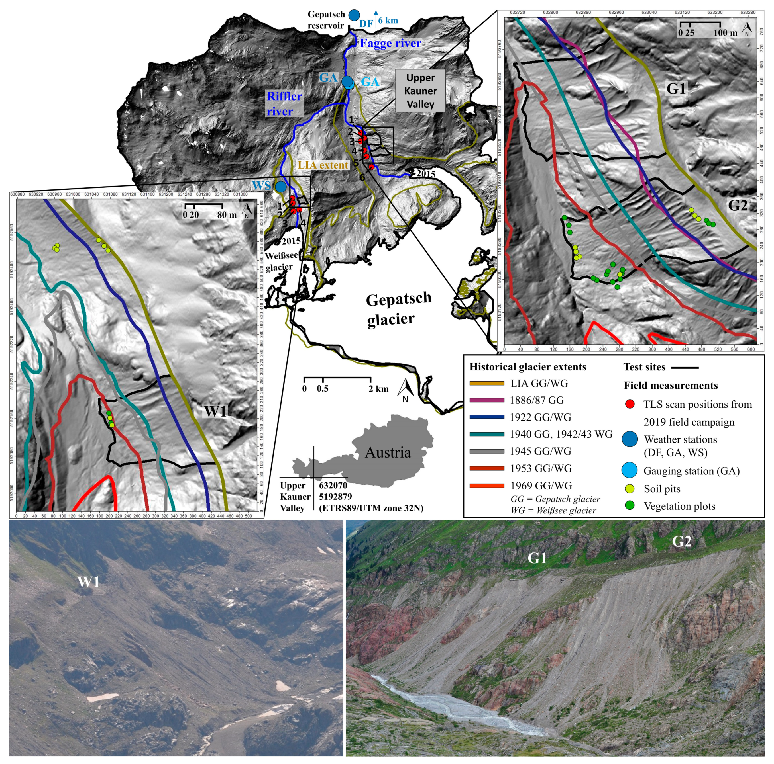Due to the good data basis (e.g., maps, terrestrial, and aerial images/orthophotos) of these glaciers since the end of LIA, the glacier extents could be continuously documented for the last decades (Figure 1). The three test sites are located on the lateral moraines of the Gepatsch glacier (named G1 and G2), drained by the Fagge River, and the Weißsee glacier (named W1), drained by the Riffler River (a tributary to the Fagge River). The test sites are characterised by intense paraglacial morphodynamics and low vegetation cover. The material of the slopes can be described as typical moraine material, which is unsorted and contains grain sizes from silt to boulders. The valley belongs to the inner-alpine dry province and is described as a continental one with low mean annual precipitation values and is one of the driest regions of the Alps [26,90]. Figure 1 and

Table 1. Characteristics of the test sites. Values were derived from the 2019 DEM (Section 3.1).

Test Site	Location (Centre) (ETRS89/UTM Zone 32N, EPSG Code: 25832)	Aspect	Range of Elevation (Ellipsoidal Heights) (m)	Size (km²)	Max. Slope Length (m)	Mean (and Max.) Slope Gradient (°)	Start of Deglaciation	Completely Deglaciated between (See Figure 1)
G1	E 632864	W	2070–2280	0.081	330	33.95 (ca. 75)	End of LIA/~1855	1953 and 1969
	N 5193652
G2	E 633000	W	2090–2360	0.066	370	35.07 (ca. 75)	End of LIA/~1855	1953 and 1969
	N 5193307
W1	E 631170	W	2600–2730	0.033	170	33.40 (ca. 70)	End of LIA/~1855	1953 and 1969
	N 5192139

give an overview.

3. Materials and Methods

3.1. Photogrammetric and LiDAR Data Collection, Processing, and DEM Generation

For the generation of the historical DEMs (1970 and 1971), digital historical aerial images were used, which were provided by the Office of the Tyrolean Government, Department of Geoinformation (Tyrol, Austria). The digitized images (scanning resolution: 12 µm) were provided in TIFF format together with the corresponding calibration protocol of the camera [97,98]. The flights on 29 September 1970 covered the northern part of the Upper Kauner Valley including the Gepatsch glacier forefield (test sites G1/G2) and on 18 August 1971 covered the southern part of the Upper Kauner Valley including the Weißsee glacier forefield (test site W1) (Figure 2/

Table 2. Overview of the acquired historical images for the generation of the point clouds and the corresponding DEMs by photogrammetry/SfM [97,98,101,102].

	Northern Part of Upper Kauner Valley (Including Gepatsch Glacier Forefield/Test Sites G1 and G2)	Southern Part of Upper Kauner Valley (Including Weißsee Glacier Forefield/Test Site W1)
Purpose/Source	Tyrolean state Surveying flight/Office of the Tyrolean Government (Department of Geoinformation)	Tyrolean state Surveying flight/Office of the Tyrolean Government (Department of Geoinformation)
Date of acquisition	29 September 1970	18 August 1971
Flying altitude (m a.s.l)	ca. 8665	ca. 5025
Camera	Wild RC5/RC8	Wild RC5/RC8
Number of images	26	31
Focal length (mm)	210.43	209.48
Scanning Resolution (µm)	12	12
Coverage area (km2)	21.7	25.4
Point density (points/m2)	8.59	8.98
Ground resolution (cm/pix)	19	17
RMS reprojection error (pix)	0.863	0.438

). The historical images were processed in Agisoft Metashape Professional software package (https://www.agisoft.com/; software version: 1.5.5.9097), which allows the use of fiducial marks for the camera orientation.

The following pre-processing steps were performed. Since the scanned images have a slightly different number of pixels, all images from the same camera were resized to share the same size. Since the images from 1970 and 1971 were jointly oriented, but taken by different cameras with different focal lengths (Table 2), it was ensured that the resolution differed by at least one pixel. In a second step, the black border of each image with the camera metadata information was masked as it may interfere with the orientation of the camera [99]. Third, after entering the calibrated focal length for both cameras, the fiducial marks were automatically detected by the software. A manual adjustment of the centres was required for few fiducial marks. The definition of the camera geometry was set by reporting the coordinates (x, y) of the fiducials (mm) with the corresponding sign. After defining the coordinate system (ETRS89/UTM zone 32N; EPSG code: 25832) with ellipsoidal heights, the processing steps consist of (i) the initial joint orientation of the 1970 and 1971 images, (ii) the selection of the ground control points (GCP) in the images with their corresponding global coordinates, (iii) the final camera orientation (bundle block adjustment) including scale definition, (iv) the dense point cloud computation based on dense image matching, and (v) the generation of the orthophoto. The steps (iv) and (v) were performed separately for the 1970 and 1971 datasets. Based on aerial images provided by the Austrian Federal Office of Surveying and Metrology (BEV), orthophotos of 1953 (for glacier extent mapping, Section 2) and 2015 (for vegetation mapping, Section 3.3.1 and Section 4.2.1), were created using the same workflow.

The approach used required a high number of ground control points (GCPs) covering the entire Upper Kauner Valley with high accuracy. Since this includes hardly accessible high alpine terrain, the coordinates of the GCPs were extracted from an ALS data set. The selection of these 101 GCPs was done on well recognizable structures and stable areas, such as rock formations, which could be identified in the aerial photographs as well as in the ALS point cloud, as shown in Figure 2. For this purpose, the most recent available ALS data set was taken, which was obtained in 2017 as part of the PROSA project (“High-resolution measurements of morphodynamics in rapidly changing PROglacial Systems of the Alps”). The data was taken from a helicopter and a mounted VP1 (VuxSys LR) mobile laser scanner from Riegl (Riegl.com). This flight mission was performed by the Chair of Physical Geography at the Catholic University of Eichstätt-Ingolstadt at an average flight altitude of 150 m meters above ground and a laser impulse measuring frequency of 200 kHz, with a resulting point density of 5.8 points/m². This data set was available in ellipsoidal heights. The generated point cloud was pre-processed by an automatic strip adjustment and georeferencing [100].

Furthermore, the ALS data set acquired in 2006 was used (data acquisition: 5 September 2006, average point density: 4.6 pts/m², coordinate system: ETRS89/UTM Zone 32N, EPSG code: 25832), which was provided by the Tyrolean Hydropower AG (TIWAG, Austria, Innsbruck) for this study as part of the SEHAG project (“Sensitivity of High Alpine Geosystems to Climate Change since 1850”) of the Chair of Physical Geography at the Catholic University of Eichstätt-Ingolstadt and covers the entire Upper Kauner Valley. This dataset was also pre-processed by an automatic strip adjustment and georeferencing [100].

The data of 2019 were collected with a TLS VZ-4000/Riegl (Figure 3). The test sites on the Gepatsch moraine were scanned on 25 June 2019 (6 scan positions) and those on the Weißsee moraine on 26 August 2019 (4 scan positions (Figure 1). The scans were performed with a laser pulse repetition rate of 30 kHz, which corresponds to an effective measurement rate of 23,000 pulses per second [103]. The single scans were acquired in the local coordinate system of the TLS. The technical specifications of this panoramic TLS are shown in

Table 3. Technical specifications of the TLS VZ-4000 from Riegl [103].

Laserscanner	Laser Wavelength	Max. Range (m)	Beam Divergence (mrad)	Accuracy (mm)	Precision (mm)	Max. Data Acquisition (meas./s)
Riegl VZ-4000	Near infrared	4000	0.15	15	10	222,000

.

The single terrestrial scans were processed with the software RiScanPro (Riegl.com). To reduce the number of acquired points to the necessary ones, all redundant and flying points were removed manually in a first pre-processing step. In a further step, the scans were co-registered using the software features coarse registration via point pairs (GCPs) and the subsequent Multi Station Adjustment (MSA), which adjusts two point clouds to each other in several iterations by a software intern algorithm (fine registration). For this purpose, stable areas (mostly bedrock adjacent to the test sites) were cut out of the 2017 ALS data set. Afterwards, the coarse registration was performed via point pairs from the 2017 ALS dataset and the 2019 TLS dataset using the master scan (scan no. 4 at G1/G2 and scan no. 2 at W1) and the depending slave scans. For every single scan, a minimum of 9 and a maximum of 11 point pairs (GCPs) were selected, which were evenly distributed over the respective scans. A mean standard deviation of 0.21 m was achieved for the point clouds of the Gepatsch test sites and 0.34 m for the Weißsee test site. After this coarse registration, a fine registration using the MSA algorithm in RiScanPro was performed. The iterative adjustment results in a mean standard deviation of 0.0194 m at the test sites G1/G2 and 0.0164 m at the test site W1 of the Weißsee glacier forefield.

All point clouds were then prepared for the conversion into digital elevation models (DEMs). These preparatory steps included the removal of outliers and the generation of homogeneous point clouds by block thinning, since the density of the point could influence the accuracy of the DEM. Additionally, the vegetation in the 2019 TLS point cloud was removed by ground classification. The point clouds were then converted to DEMs with a cell size of 1 m. These steps were performed in SAGA LIS (Laser Information System; Laserdata.at).

3.2. DEM of Difference (DoD) Analysis

3.2.1. Derivation of Test Sites and Morphological (Sediment) Budgets Analysis

For the exact investigated test sites (AoI), polygons were created, which were selected under the following conditions. While the upper boundary of the test sites was fixed defined by the maximum LIA glacier extent, the lateral boundaries of the test sites varied between the periods, as these are based on a hydrological flow routing algorithm (D8) [104] on the corresponding DEMs, which may change slightly due to hydrological and geomorphological processes on the slopes between the time steps or due to the quality of the individual DEMs. Therefore, it cannot be excluded that sediment has reached the test sites from outside. For example, while the upper boundary of test site G2 is a morphologically shaped watershed (LIA/~1855 glacier extent, see Section 2/Figure 1), small parts of G1 and W1 are physically connected to rock areas further up, which are located outside the mapped lateral moraine and thus outside of the defined areas of interest. However, this influence is considered as minor. Moreover, the underlying streams play an important role in the development of the slope test sites, as the slope–channel contact line changed, e.g., due to undercutting by the main channel, sediment input from slopes or alluvial deposits. Therefore, the lower vertical boundaries of the test sites were also subject to variations. For these reasons, the extent of the test sites varies slightly between the different periods.

To generate the DoD, the individual DEMs were subtracted from each other so that the height changes (positive or negative) of each cell could be determined (Equation (1)):

$${\mathrm{DoD}}_{2019/2006}={\mathrm{DEM}}_{2019}-{\mathrm{DEM}}_{2006}{ \mathrm{and} \mathrm{DoD}}_{2006/1970,1971}={\mathrm{DEM}}_{2006}-{\mathrm{DEM}}_{1970,1971}$$

(1)

Then the (i) negative and (ii) positive subsets of each DoD were separately added up to calculate the volume of erosion or deposition (Equation (2)) for each test site and period (1970/1971 to 2006 and 2006 to 2019). The sum of (i) and (ii) gives the net volumetric sediment balance.

$$\mathrm{V}=\mathsf{\Sigma } \mathrm{DoD}\times {\mathrm{L}}^2$$

(2)

where Σ DoD is the sum of the corresponding DoD subset and L is the raster cell size (1 m). For the exact volume computation, the first polygon was used, e.g., for the DoD_{2019_2006} the polygon from 2006.

3.2.2. Uncertainty Assessment of Sediment Balancing

The presence of uncertainty in the individual DEMs and the resulting DoD leads to uncertainty in the morphological sediment volume computations [22,105,106]. Furthermore, DEMs of different survey techniques were used, which leads to different types of errors in the individual DEMs [107,108,109,110]. For the computation of errors and uncertainties in DEMs or DoD, reference data sets or direct repeat measurements can be used [111]. As none of these were available due to the study design, the uncertainty of all DoDs was estimated directly at stable areas, which were assumed that no changes occurred there during the whole investigation period (Figure 4 and Figure 5). The areas used for the error estimation were randomly selected within the identified areas and were about 1% of the size of the corresponding test sites. However, for reasons of comparability, equally large stable areas of the test sites were selected in both periods. Their locations are shown in Figure 5 (red rectangles), which are either directly on the test sites or very close to them. To determine and exclude error values and uncertainty from DoD, several studies apply a minimum Level of Detection (_minLoD) [105,112,113].

For the uncertainty estimation of the sediment balance, the approach recommended by Anderson (2019) [114] was followed, who concluded that the exclusion of DoD values of a certain _minLoD should be applied when calculating erosion and accumulation volumes separately, but should not be applied when estimating the net change, as these are not significantly affected by the same random errors and the positive and negative error values can cancel each other out to a large extent. Since very long periods have been analyzed on highly active slopes with high surface changes, it is unlikely that random errors will reverse the sign of the real changes. Therefore, this study refrained from removing values below a certain threshold from the DoDs for the uncertainty assessment of the sediment balancing and instead specified an uncertainty value for the calculated net volume changes. Figure 4 shows the arithmetic mean, accuracy (RMSE), and precision (standard deviation) of the determined stable areas. Since the mean values of the stable areas are very close to zero, a normal distribution can be assumed and a systematic error (as, e.g., by slightly tilted scans) is excluded. Moreover, the Lilliefors (Kolmogorov–Smirnov) test was applied in R to prove the normal distribution (Figure 4). The analysis of the error propagation of the volume calculation is based on the assumption of independence.

Using variogram analyses in R, both spatially correlated and uncorrelated random errors were identified. The variogram analyses show that the stable areas of the DoDs based on the DEMs 1970/1971 (photogrammetry) and 2006 (ALS) have a spatially correlated random error due to the nugget effect (stable areas 1 and 3: 0.02, stable areas 5: 0.01), while the DoDs based on the DEMs 2006 (ALS) and 2019 (TLS) have an uncorrelated random error due to the pure nugget effect. In general, DoDs based on ALS and TLS DEMs are less prone to errors and uncertainties than DoDs that comprise a photogrammetry derived DEM (Figure 4). For the spatially correlated random errors of the stable regions (DoD_{2006_1970/1971}), the theoretical variogram was adjusted to the point sample of the DoDs.

The following equations were used to determine the total volumetric error [114]:

In case of spatially correlated random error (Equation (3)) [114]:

$${\mathsf{\sigma }}_{\mathrm{v}, \mathrm{sc}}=0.79{\mathrm{a}}_{\mathrm{i}}\sqrt{\mathrm{n}}{\mathrm{L}\mathsf{\sigma }}_{\mathrm{sc}}$$

(3)

where ${\mathrm{a}}_{\mathrm{i}}$ is the circular area over which errors are correlated (a = semivariogram range, spherical model, no nugget), $\mathrm{n}$ is the number of cells being aggregated, $\mathrm{L}$ is the cell size (m²), and ${\mathsf{\sigma }}_{\mathrm{sc}}$ the spatial correlated DoD uncertainty (m).

In case of uncorrelated random error (Equation (4) [114]):

$${\mathsf{\sigma }}_{\mathrm{v}, \mathrm{re}}=\sqrt{\mathrm{n}}\mathrm{L}2{\mathsf{\sigma }}_{\mathrm{rms}}$$

(4)

where $\mathrm{n}$ is the number of cells being aggregated, $\mathrm{L}$ the cell size (m), and ${\mathsf{\sigma }}_{\mathrm{rms}}$ the RMSE.

Nevertheless, for cartographic representations (Figure 5), the _minLoD was calculated [105,112,113], using the same stable areas. This approach assumes that random uncertainty has an expected value of 0 and is normally distributed with a standard deviation equivalent to the standard deviation of error ${\mathsf{\delta }}_{\mathrm{DoD}}$ measured at stable areas. Under this assumption, a critical t value ${\mathrm{t}}_{\mathrm{crit}}$ can be selected from Student’s t distribution to set up a confidence interval 0 ± t * ${\mathsf{\delta }}_{\mathrm{DoD}}$ containing, at a given confidence level, DoD values measured when in fact no change has occurred on a raster cell. The _minLoD was determined with a confidence level of 95% (${\mathrm{t}}_{\mathrm{crit}}=1.96;$ Equation (5)).

$${}_{\min }\mathrm{LoD}={\mathrm{t}}_{\mathrm{crit}}\times {\mathsf{\delta }}_{\mathrm{DoD}}$$

(5)

Therefore, the cells with |DoD|<${}_{\min }\mathrm{LoD}$ in the DoD maps were masked (Figure 5).

3.3. Collection and Analysis of Field Data

3.3.1. Type of Vegetation and Soil Analysis

The plant communities of the test sites were analyzed in ArcGIS (version 10.6.1), based on the generated orthophoto of 2015 (Section 3.1). Polygons of the different landcover types were drawn manually and the percentage of each type was calculated. To validate the landcover types and to investigate the role of vegetation on the morphodynamics at the test sites, vegetation surveys were performed in July 2020. On 18 plots (2 × 5 m), total cover of the vegetation was estimated, and plant communities were defined (Figure 1). Two plots were located at test site W1 in the accumulation zone. All other plots (16) were located at test site G2, seven in the accumulation zone, some of them with ongoing erosion processes. Six of the plots were in the lower erosion zone and three above the erosion area.

In August 2020, 16 soil pits were excavated in moraine material at exposed eroded areas (6 soil pits), as well as in deposited moraine material (10 soil pits) on the test sites of both glacier forefields (Figure 1). The locations were chosen on the basis of their significance (erosion or deposition areas) and accessibility in the terrain. Since the erosion area of W1 was difficult to access due to very steep terrain, an additional and comparable erosion area close-by was analyzed instead. To determine the input from the slopes into the channels, wet bulk density was determined at a depth of 0–10 cm in the field by excavating a total defined volume of 7000–12,000 cm³ per site. The material was sieved to 2000 mm, 630 mm, and 2 mm. From the fine material <2 mm, particle size distribution was determined using laser diffraction (Malvern Mastersizer 3000).

3.3.2. Meteorological and Hydrological Data

To investigate the influence of changing external factors, such as precipitation on the morphodynamics of the test sites, data from three meteorological stations, which were maintained and provided by the TIWAG, were analyzed. These include the stations “Dammfuss (DF)”, “Gepatschalm (GA)” and “Weißsee (WS)”. The three weather stations collect temperature and precipitation data in 15-min intervals.

Table 4. Overview of the data recorded from the weather and gauging stations and their locations.

Weather and Runoff Station	Period of Available Data	Elevation (m a.s.l.)	Location (ETRS89/UTM Zone 32N, EPSG Code: 25832)	Linear and Flow Distance to the Test Sites (km)
Weather station				Linear distance to the test sites
Dammfuss (DF)	1 January 1988–31 December 2019	1770	E 632260,	8.7 to G1, 8.9 to G2 and 10.2 to W1
			N 5202225
Gepatsch Alm (GA)	1 August 2009–31 December 2019	1900	E 632251,	1.5 to G1, 1.9 to G2 and 3.1 to W1
			N 5195058
Weißsee (WS)	1 December 2006–31 December 2019	2540	E 630648,	2.5 to G1, 2.5 to G2 and 0.6 to W1
			N 5192468
Gauging station				Flow distance to the test sites
Gepatsch Alm (GA)	1 January 1971–31 December 2019	1895.01	E 632330,	1.6 to G1, 2.1 to G2 and 4.1 to W1
			N 5194957

and Figure 1 show the location, elevation, and the distance of the stations to the individual test sites. The comparison of the distance shows that the weather stations GA and WS have the shortest distance to the test sites but the recording time of these stations only covers the period from 2006 to 2019. The DF station, on the other hand, has been measuring precipitation and temperature data since 1988, but is located about 6 km north of the entry of the Fagge River into the Gepatsch reservoir below the dam and thus furthest away from the test sites and at a considerably lower elevation than the other weather stations.

The resulting 18-year gap of 1988 (start of DF recording) and 1970 (start of morphodynamic analysis) is partly covered by the GA gauging station, which has been measuring runoff in Upper Kauner Valley since 1971 and allows to conclude on higher rainfall events. Due to numerous gaps in the first half of the 1970s, this time series was not analyzed until 1977, leaving a gap of 7 years until the beginning of the morphodynamic analysis in 1970. The station is located behind the confluence of the Fagge and the Riffler rivers, and thus includes the discharge of both glacier forefields and all test sites. Other available weather stations with a longer recording period were not included in this study, since they are located in neighbour valleys or at much lower elevations and record only at hourly or daily intervals, leading to uncertainties too large for the analysis of the morphodynamics in this study.

To analyse the data of the weather stations, mean annual temperature, mean annual precipitation sum, and annual and total trends based on these, were calculated. These calculations only include fully available years (1st of January to 31st of December), so 2009 for GA and 2006 for WS were not included in these calculations, as the measurement started in the current year. For the analysis of the individual precipitation events, different classes, which are defined by the amount of precipitation, were calculated. In addition to the short-term 15-min precipitation events, also 1-h events were analyzed (using a moving window of the 15-min intervals). The 15-min events were divided accordingly into classes with 2.5 mm intervals (0–2.5; 2.5–5; ...) and the one-hour events in 5-mm intervals (0–5; 5–10; ...). In addition, the daily sums of precipitation were analyzed to investigate the change of long-term precipitation events.

A trend analysis based on the Mann–Kendall test was also carried out for the time series of the gauging station GA, based on the maximum hourly values. In addition, the data of the gauging station were examined for discharge peaks in the different periods. Moreover, all events (mean hourly discharge) in the respective months were plotted in order to classify them seasonally.

Where possible, the respective time series of the weather stations (DF: 1988–2019) and the gauging station (GA: 1977–2019) were divided on 5 September 2006, the date of generation of the 2006 ALS point cloud and thus the separation of the defined periods in this study. All analyses were performed in R.

4. Results

4.1. Surface Change Detection Analysis and Morphological Sediment Budgets

Figure 5 and Figure 6 show the computed morphological sediment budgets for all test sites in the respective periods. In the following, the period between 1970/1971 and 2006 is defined as the first and the period from 2006 to 2019 as the second period. A distinction is made between sediment sources (red), sediment sinks (blue), and the resulting net balances (grey). The height changes determined by the DoDs show clear differences both at the different test sites and within the different periods. As different periods were compared, in addition to the total sediment budgets, mean annual volume changes were also given for comparison.

Based on the DoDs, geomorphological processes can be separated and analyzed (Figure 5). The test sites G1 and G2 are characterised in the upper parts by a clear headcut retreat and gully incisions in the first period, which continues in the second period and is caused by fluvial processes like gully erosion, slope wash, and gravitational processes such as slope failure (sidewall collapse) and debris flows. Analysing the erosion and accumulation forms and the resulting high height differences (maximum height differences: −28.6 m/+7.7 m), a landslide could be identified in the first period at G1. In addition to this high negative vertical change, there was also a 60-m-long horizontal change of the erosion area (headcut). Certain parts of these height changes may also have been caused by other geomorphological processes during the 36 years, but the main part of these changes can be clearly attributed to a landslide. The middle and lower parts of the slopes are characterised by deposition areas and levées. Therefore, the eroded material has been deposited downslope or downstream. In the lower third of the test site, erosion processes led to the formation of alluvial fans and debris cones. Especially in the second period, lateral erosion occurs due to the process of undercutting by the main rivers, which led to a reduction of the slope length over the entire test sites (G1 total erosion: 2165 m³/total deposition: 16 m³; G2 total erosion: 3072 m³/total deposition: 1289 m³). In the first period, changes of the alluvial fans and debris cones can be detected (slope expansions and reductions) (G1 total erosion: 3 m³/total deposition: 3937 m³; G2: 19 m³/total deposition: 778 m³). In addition, the presence of dead ice in the first period of G2 was detected (maximum height change: −12.4 m), due to a rounded lowering of the terrain and no corresponding accumulation changes, and thus could not be classified as a geomorphological process. Finally, the values of the volume changes at the foot of the slopes (undercutting by the main rivers) as well as those of the dead ice were excluded from the morphological sediment budget, which therefore only include those of the morphodynamics on the slopes.

In contrast to the test sites on the lateral moraine of the Gepatsch glacier, W1 shows clearly less morphodynamics. In the first and second period, W1 was mainly affected by fluvial erosion and debris flows, resulting in different accumulation areas on the upper and lower parts of the slope. W1 was affected by considerable dead ice thawing during the first period, which caused negative terrain changes down to −10.2 m and again no corresponding accumulation zones. This is the maximum height change on this test site during the investigated period. During the first period, also lateral erosion along the entire foot of the slope occurred, as well as the deposition of alluvial material (W1 total erosion: 510 m³/total deposition: 1374 m³). In the second period, a landslide (maximum −6.5 m) was triggered upslope the thawing dead ice area of the first period, which formed a clearly visible debris cone (maximum +5.1 m). A direct connection between the thawing of the dead ice and the landslide on test site W1 can be assumed, as the dead ice zone subsided by more than 10 m in the first period and therefore became steeper, which probably led to an instability of this part of the lateral moraine. In addition, the test site above the landslide is physically connected to rock areas above the max. LIA glacier extent and thus could have been caused by a rainfall event, due to the large hydrological catchment area. The landslide has an immense influence on the mean annual erosion and accumulation volumes of the second period, compared to the first, as this single process led to a clear increase in the mean annual erosion and accumulation volumes of the whole period. The formation of a huge accumulation zone led to a lengthening of the slope and a shift of the channel, while at the same time lateral erosion by the main river reduced the length of the slope directly next to the formation of the debris cone (Figure 5; W1 total erosion: 387 m³/total deposition: 2 m³). Dead ice areas on the slopes and lateral erosion (undercutting), as well as alluvial deposits on the lower part of the slopes, were as well excluded from all sediment computations.

Test site G1 shows a 75% decrease in the mean annual erosion and a 71% decrease in the mean annual deposition volumes in the second period compared to the first period. The total sediment budget changed from −50,134 m³ (+/−640 m³) to −2700 m³ (+/−17 m³). This leads to an 85% reduction of the mean annual net balance from −1393 m³ to −207 m³ and to the fact that 31% in the first period and 19% in the second period of gross erosion were exported from this test site. Similar to G1, G2 also shows a clear decrease from the first to the second period of erosion and deposition. There is a 49% decrease in mean annual erosion and a 22% decrease in deposition, resulting in a 65% reduction in mean annual net balance from −1719 m³ to −610 m³. Of this test site, 65% of gross erosion was exported from the test site in the first period and 46% in the second period. The total sediment budget changed from −61,876 m³ (+/−455 m³) to −7937 m³ (+/−34 m³). In contrast to G1 and G2, W1 shows a 54% increase in the mean annual erosion and 76% in the mean annual deposition in the second period compared to the first. This leads to a 3% reduction of the mean annual net balance from −224 m³ to −218 m³ and to the fact that 61% in the first period and 27% in the second period of the gross erosion were exported from this test site. This leads to a change of the total sediment budget from −7857 m³ (+/−136 m³) to −2837 m³ (+/−10 m³). In summary, the net balance is entirely negative for all time periods and test sites and is clearly lower in the second period compared to the first on the test sites G1 and G2. In contrast, the mean annual erosion volumes and the mean annual deposition volumes at W1 have increased, which leads to a net balance remaining at a similar level (Figure 5 and Figure 6).

4.2. Field Data

4.2.1. Type of Vegetation and Soil Analysis

The test sites are mainly characterised by scree (72–93%), which is forming the erosion and deposition areas (

Table 5. Landcover classes and their relative spatial extents of the test sites (%).

Landcover Classes (Type of Vegetation)	G1	G2	W1
Scree	27.3	12	16.8
Scree community 1–6% cover	37.6	55	55.6
Scree community ≤60% cover	12.1	3.8	21.3
Alpine grassland	0.6	2.6	2.3
Shrub	1.3	3.3	0.2
Dwarf shrub rich grassland	14.6	14.7	0
Dwarf shrub	1.4	2.8	0
Shrub with trees	0	0.4	0
Bedrock (Paragneiss/Orthogneiss)	5.3	5.7	3.8
Total	100	100	100

/Figure 7). Small parts are covered by bedrock (Paragneiss/Orthogneiss, 4–6%). The upper part of the erosion areas of G1 and G2 are completely free of vegetation or have a low cover (1–6%). Above the erosion areas, a dwarf shrub rich grassland and dwarf shrub communities occur. The deposition areas of G1 and G2 are characterised by different colonisation stages. According to erosion/deposition events in different years, a variety of scree communities with low and high vegetation cover prevails. However, on the stable parts, shrubs dominate. At G2, some of these parts are enriched by trees (Larix decidua, Betula pendula, and Populus tremula). The test site W1 is dominated by scree communities, mainly with 1-6% cover. Only on the edges of the test site, alpine grassland occurs.

The moraine material consists of non-stratified material from silt to boulders. In comparison to this, the deposited moraine material consists of significantly more coarse gravel, but less medium or fine gravel, silt, and clay (

Table 6. Particle size distribution of moraine material from erosion and deposition area.

	Moraine Material		p-Value (Wilcoxon)	Mean
	Erosion area	Deposition area
Moraine material (mass-%)
Coarse gravel/cobbles	4.40	37.71	0.001	16.89
Medium gravel	43.03	23.54	0.011	35.72
Fine gravel	19.85	12.66	0.007	17.16
Fine soil	32.72	26.08	0.428 (n.s.)	30.23
Fine soil texture (vol-%)
Sand	50.08	64.35	0.013	58.24
Silt	48.76	34.91	0.020	40.84
Clay	1.15	0.73	0.039	0.91
Bulk density (t m−3)	1.813	1.994	0.385 (n.s.)	1.926

). We attribute the unexpected lower bulk density of the moraine material in the erosion areas compared to the accumulation areas to the fact that the moraine material in the uppermost areas, where the soil pits were taken, were not under the great pressure of the glacier, like middle or lower areas of the lateral moraines. However, the bulk density of the deposited moraine material did not significantly differ from the original moraine material. For this reason, all following volume-to-mass conversions were performed using a mean bulk density of 1.926 t m⁻³ (Table 6). The computed sediment input from the slopes into the channels is shown in Figure 8. The calculation is based on the corresponding net balance, which was exported from the defined test sites in the corresponding periods (Figure 5 and Figure 6). A comparison of the periods shows a general decrease in sediment input between the two periods, a clear decrease for G1 (>85%) and G2 (>65%) and a small decrease for W1 (<3%), although this can also be described as a similar level (Figure 8).

4.2.2. Meteorological and Hydrological Regime

Due to their location, elevation and measurement period, the weather stations show clear differences in mean annual temperature, mean annual precipitation sum and precipitation patterns (

Table 7. Mean annual temperature values and the corresponding trend analyses in the measuring periods of the weather stations.

Weather Station	Mean Annual Temperature (°C)	Annual Temperature Trend	Total Temperature Trend (°C)
Dammfuss (DF)	4.48	y = 0.01x+4.38	+0.21
Gepatsch Alm (GA)	2.72	y = 0.1x+2.28	+0.97
Weißsee (WS)	−0.11	y = 0.08x+(−0.59)	+1.05

/Figure 9). In general, the analyzed weather station data indicate an increase in temperature. The annual trend is +0.01 °C/year for DF (32 years), +0.1 °C/year for GA (10 years), and +0.08 °C/year for WF (13 years), which results in a total temperature increase of +0.21 °C (DF), +0.97 °C (GA) and +1.05 °C (WS) in the respective periods (Table 7). In contrast, the mean annual trends of the corresponding precipitation sums show differences, since precipitation decreases at the stations DF and GA in the corresponding periods, but increases at WS, with annual trends of −0.42 mm/year (DF, 32 years), −12.52 mm/year (GA, 10 years), and +7.99 mm/year (WS, 13 years), respectively (Figure 9).

The different classes of precipitation events, categorized into precipitation amounts (

Table 8. Short- and long-term precipitation events of the (if available) first and the full second period of the weather station DF.

Precipitation Interval 15 min (mm)	1 January 1988–5 September 2006		5 September 2006–31 December 2019		Change (%) (Based on the Mean Annual Number of Events)
	No. Events	No. Events %	No. Events	No. Events %
0–2.5	49,095	7.56	36035	7.7313	+1.6
2.5–5	216	0.033	122	0.0262	−21.8
5–7.5	47	0.0072	16	0.0034	−52.9
7.5–10	9	0.0014	4	0.0009	−38.5
10–12.5	14	0.0022	2	0.0004	−80.2
12.5–15	3	0.0005	1	0.0002	−53.8
15–17.5	2	0.0003	0	0	−100
17.5–20	2	0.0003	0	0	−100
20–22.5	0	0	0	0	0
22.5–25	1	0.0002	0	0	−100
25–27.5	1	0.0002	0	0	−100
Precipitation interval 1 h (mm)
0–5	82,605	12.6131	53304	11.5733	−10.7
5–10	975	0.1489	614	0.1333	−12.8
10–15	104	0.0159	47	0.0102	−37.4
15–20	33	0.005	3	0.0007	−87.4
20–25	18	0.0027	2	0.0004	−84.6
25–30	4	0.0006	0	0	−100
30–35	2	0.0003	0	0	−100
35–40	3	0.0005	0	0	−100
Precipitation interval 24 h (mm)
0–10	3063	44.8989	1937	40.0703	−12.4
10–20	339	4.9692	258	5.3372	5.4
20–30	81	1.1873	72	1.4895	23.1
30–40	21	0.3078	18	0.3724	18.7
40–50	3	0.044	3	0.0621	38.5
50–60	2	0.0293	2	0.0414	38.5
60–70	3	0.044	0	0	−100
70–80	0	0	0	0	0
80–90	3	0.044	0	0	−100

; weather station DF), show that in the second period (from 5 September 2006 to 31 December 2019) there were clearly less short-term 15-min and one-hour events and higher daily precipitations sums compared to the first period (if available: 1 January 1988 to 5 September 2006). However, approximately 18 years are compared with approximately 13 years (Table 8). For this reason, each class also indicates the probability of a specific event occurring and the change in the mean annual number of events in the second period compared to the first period. Thus, the comparison of the 15-min precipitation events shows that in the first period there was an increase in the probability of 0–2.5 mm event, while the probability of all other classes decreased clearly.

For the 1-h events (using a moving window of 15-min intervals), a decrease in the probability of occurrence of all classified events and a decreasing change in the mean annual number of all events with increasing impact on higher values can be observed. For the daily precipitation sums, an increasing change in the mean annual number of events between 10 and 60 mm/24 h is observed, while small events (0–10 mm/24 h) and the highest events (70–90/24 h) show a decrease compared to the first period (Table 8). Thus, in the years 2007–2019, the average annual precipitation is higher than between 1988 and 2006 (Figure 9a).

The analysis of the gauging station shows an increasing annual trend of 0.35 m³/s year⁻¹ and, over the entire period of 43 years (1 January 1977–31 December 2019), a total increase of 15.05 m³/s of the maximum hourly runoff (Figure 10a). The result of the Mann–Kendell trend test for maximum hourly runoff shows a statistically significant trend with a two-sided p-value of <0.01. An increase can also be observed regarding the frequency of higher events. For example, runoff events including all events higher than 30 m³/s (max. hourly runoff) increased by 22.6% from the first period (23 events in ~30 years (1 January 1977–5 September 2006) to 13 events in the second period (~13 years). This increasing trend of the discharge of the Fagge River (Figure 10a) can be explained mainly by the increase in meltwater due to the retreat of the Gepatsch and Weißsee glaciers. In the first period, e.g., in the years 1987 and 1988, there were extreme runoffs, which indicate corresponding precipitation events. Moreover, Figure 10b shows the mean hourly runoff (m³/s) in the respective months. In general, the highest mean discharges occurred in July, while the four highest extreme events occurred in August.

5. Discussion

Several previous studies already calculated morphological sediment budgets of test sites in the proglacial area of the Upper Kauner Valley [21,22,23,24], or e.g., in a catchment in southern Switzerland in the proglacial area of the Bas Glacier d’Arolla, Val d’Hérens [80]. However, these studies only used databases covering time ranges of months or years and not decades. 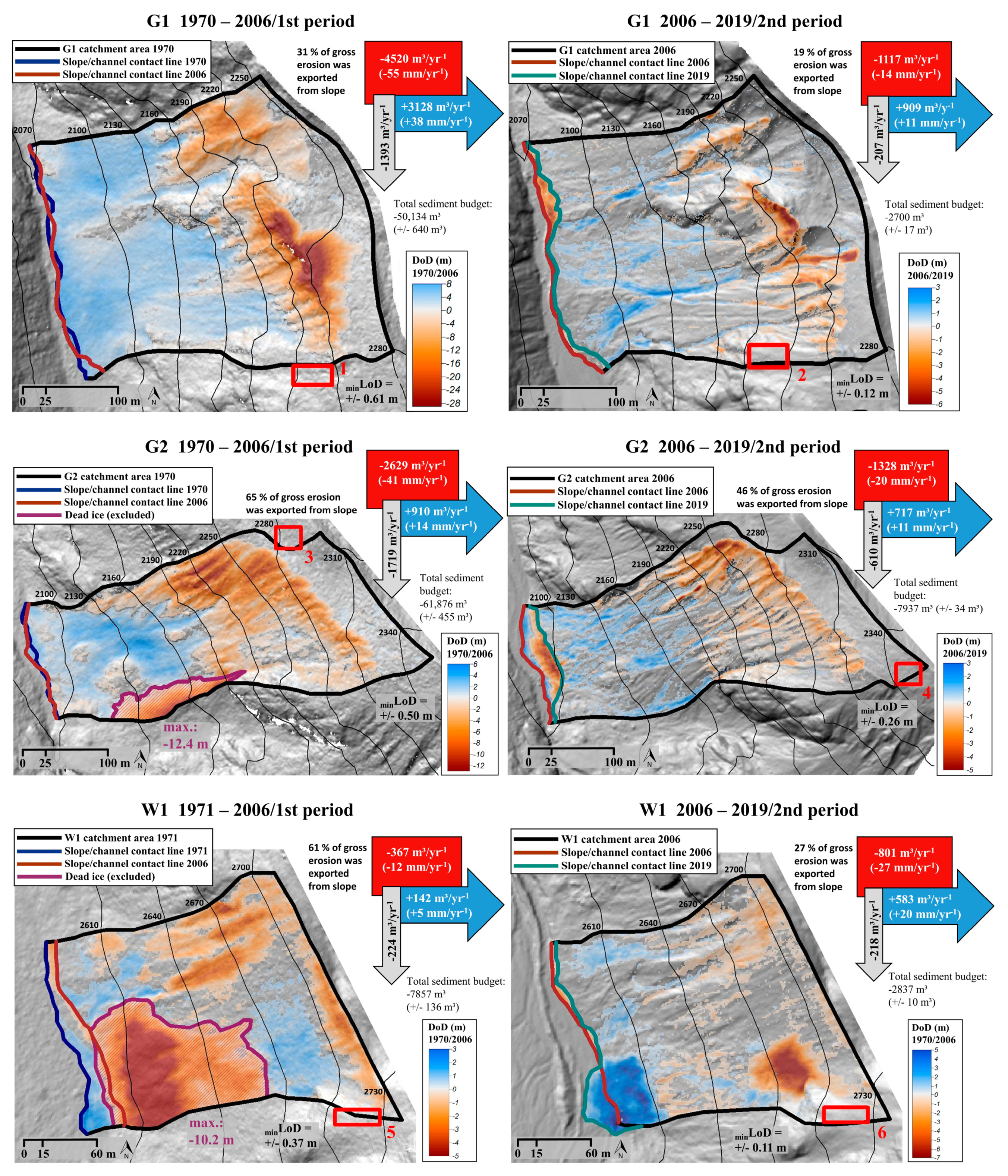The study by Heckmann and Vericat (2018) [22] shows a sediment budget for the period of 2006–2012 from the G2 test site used in this study (a slightly different area of interest). Compared to the mean annual values of this study (1970/1971–2006 and 2006–2019), the decrease in the efficiency of sediment transport of the G2 test site can be confirmed. While 66% of the gross erosion of G2 was exported between 1970/1971 and 2006 (this study), 57% was transferred to the Fagge river between 2006 and 2012 [22] and 47% from 2006 to 2019 (this study). The study by Heckmann and Vericat (2018) [22] indicates a mean annual erosion of −1384 m³ and a mean annual accumulation of +591 m³ (values were calculated on the basis of the total morphological budget given in the study), while this study (2006–2019) shows a mean annual erosion of −1343 m³ and a mean annual accumulation of +716 m³. This shows that the erosion values have not significantly changed since the work of Heckmann and Vericat (2018) [22]. Only a slight increase in accumulation can be stated. Dusik et al. (2019) [24] also calculated a morphological sediment budget of the test site G2 from 2010 to 2015 (slightly different defined test site borders). For this period, a total erosion volume of −7089.6 m³ (mean annual value: −1418 m³) and a total accumulation volume of +4122.2 m³ (mean annual value: +824 m³) are reported, which corresponds to a net balance of −2967.4 m³ (mean annual value: −593 m³), meaning that 58% of the eroded material was exported from this test site. Thus, it can be shown, that there were slight changes in the morphological sediment budgets of this test site in the period from 2006 to 2019, but that clearly less sediment was eroded in comparison to the period from 1970/1971 to 2006 (this study).

The characteristics of the test sites (in particular, size of the test site, slope length, and the mean and maximum slope gradients) have a clear influence on the morphodynamics. The differences in these are related to the fact that the glacier forefield of the Gepatsch glacier was shaped much stronger than the forefield of the Weißsee glacier due to higher glacial erosional force. As a result, the test sites G1 and G2 are larger, have longer slope lengths and have higher mean and maximum slope gradients, in contrast to W1, which probably leads to higher morphodynamics due to the higher relief energy. In addition, the higher elevation of W1 (~500 m height differences) and the associated shorter spring and summer periods, as well as the resulting longer snow cover, can reduce the vulnerability to trigger geomorphological processes, for example by precipitation events [32]. There are no differences in the deglaciation of the test sites (start of deglaciation ~1855/End of LIA and completely deglaciated between 1953 and 1969). Nevertheless, Dusik (2019) [23] identified a decrease of the morphodynamics on the lateral moraine of the Gepatsch glacier with increasing distance from the glacier by using more test sites.

Dead ice areas could be identified in the first period due to the spacious lowering of the terrain without detectable geomorphological processes. However, it cannot be guaranteed that the dead ice has been fully mapped and completely excluded from the volume calculations. For example, the “real” deposition areas may be slightly higher than shown in the DoDs, as the thawing of the dead ice may have slightly lowered the terrain. No dead ice areas were detected in the DoDs of the second period. However, the analysis of the origin of the springs which emerges from the lateral moraines of the Gepatsch glacier (including the test sites G1 and G2 of this study), by relative age dating (I¹²⁹), shows that this water originates to a certain part from dead ice remaining in the lateral moraine [56]. However, during the field work in 2019 and 2020 no exposed ice was seen on the test sites.

The mean annual erosion and accumulation volumes of these two determined long-term periods were strongly influenced by individual fluvial processes or gravitational mass movements, such as landslides. The described landslides at G1 in the first period and at W1 in the second period must be highlighted here. Due to the long periods that were compared, it is difficult to clearly define individual processes, except those which cause major surface changes like for example large landslides. Nevertheless, clear changes in the total morphodynamics and the corresponding slope channel coupling of the different test sites and in the different periods can be seen.

While at the steep test sites almost no vegetation occurred due to ongoing erosion processes, late successional vegetation was found in areas, which are more stable and have slightly lower slope gradients. This indicates that, in contrast to findings by Eichel et al. (2018) [57], slope stabilization by vegetation and related soil formation is hindered when the morphodynamic processes are too strong, and that later successional stages only start to occur at steep slopes with fewer morphodynamic processes.

Extreme rainfall events in summer play a major role in the morphodynamics, and therefore represent the most active time of sediment transport processes in alpine catchment areas [23,24,58,59]. The study by Haas et al. (2012) [21], which was also conducted on the slopes of this study (similar area of interest as G1 and G2), shows that 71% (2526.8 m³) of the material transported by debris flows between August 2010 and September 2011, which were mainly triggered by one heavy rainfall event, accumulated at the foot of the slope, whereas 29% (1033.5 m³) was transported into the Fagge River. The work of Dusik (2019) [23] shows the triggering of sediment transport processes by precipitation events on the lateral moraines of the Gepatsch- and Weißsee glaciers, with a higher temporal resolution (several years as well as seasonally), and found that heavy rainfall events lead to sediment transport processes and thus to a higher slope channel coupling. Moreover, the analysis of Dusik (2019) [23] revealed that even rainfall events of 10 mm/h are sufficient to trigger the transport of sediment on slopes and the transfer to the adjacent Fagge river. Sediment transport is highly dependent on moisture conditions, sediment availability and precipitation intensities. In addition, the spring months can create important preparatory conditions for sediment transport processes due to snowmelt on the slopes and the associated moisture [24]. 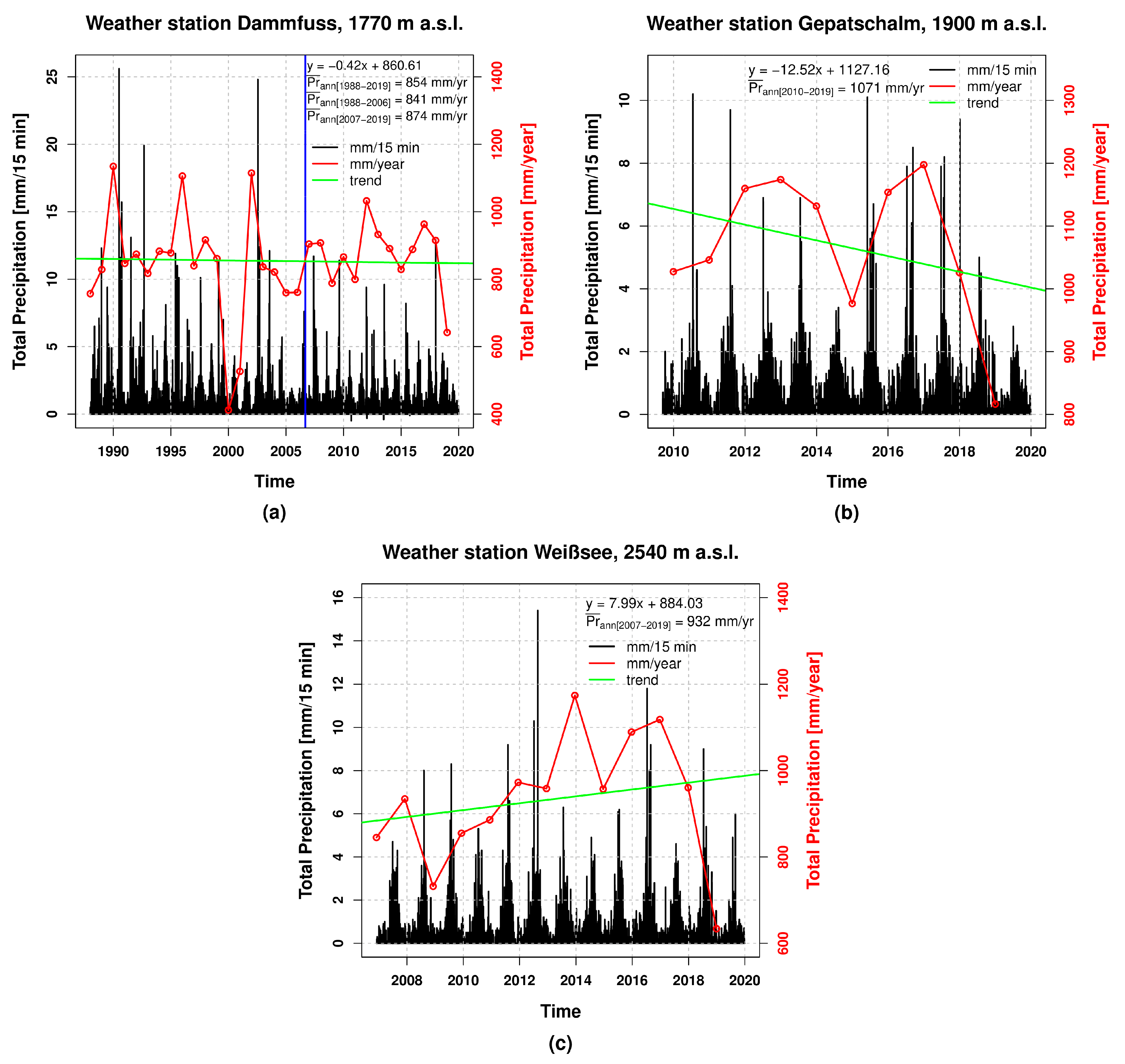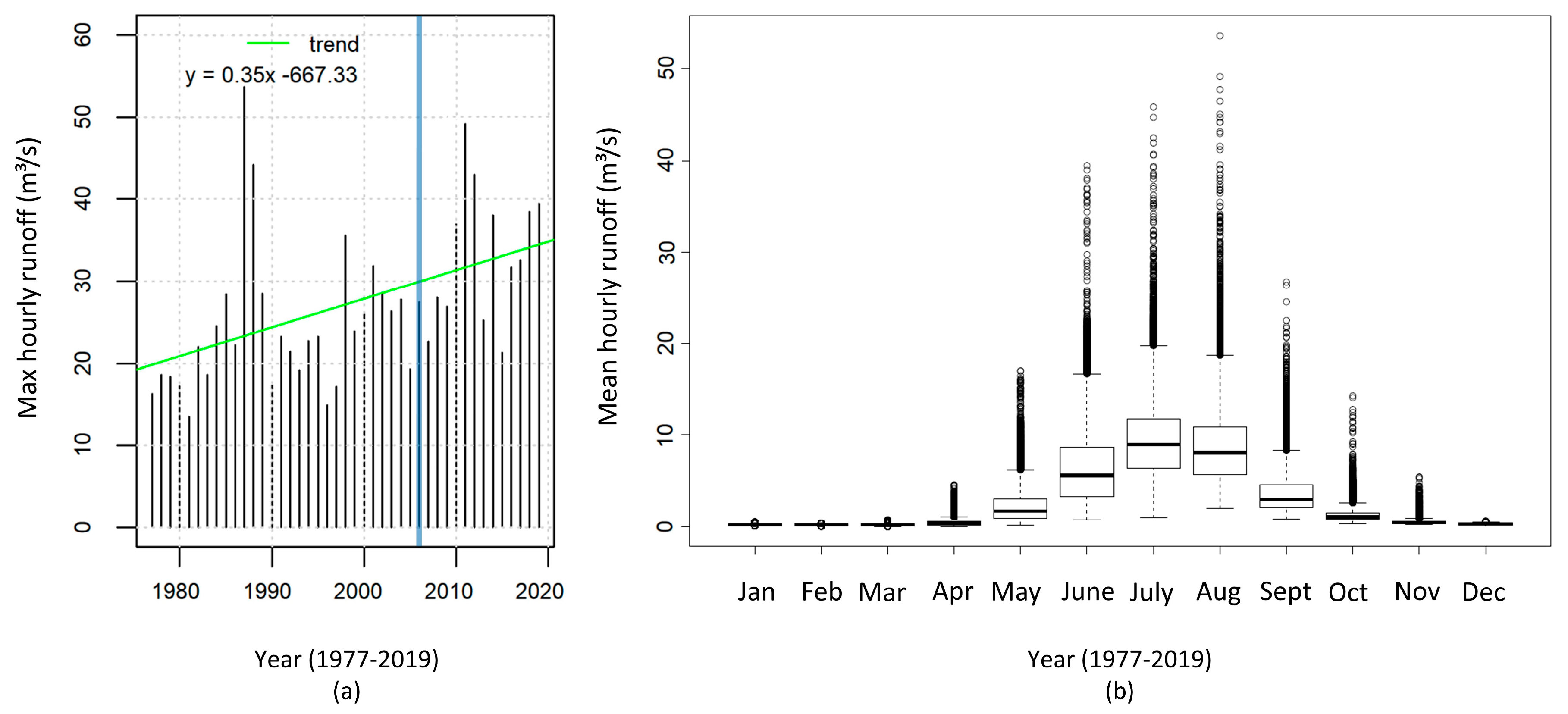A positive correlation between the number of mass movements and the number of threshold exceedances of extreme daily precipitation sums and the number of extreme precipitation intensities was detected [23]. By comparing the morphodynamics of this study within the two long-term periods with the precipitation events and with the runoff, it can be observed that the periods differ clearly regarding the morphodynamics and the meteorological and hydrological conditions. It can be assumed that there is a direct connection between the higher morphodynamics and the higher precipitation and the high runoff events especially in 1987 and 1988 and the high morphodynamics in the first period and the lower precipitation events and lower morphodynamics in the second period. Although the daily total precipitation (between 10 and 60 mm/d) of the weather station DF are increasing, the 15-min and 1-h events in particular are clearly decreasing.

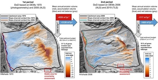
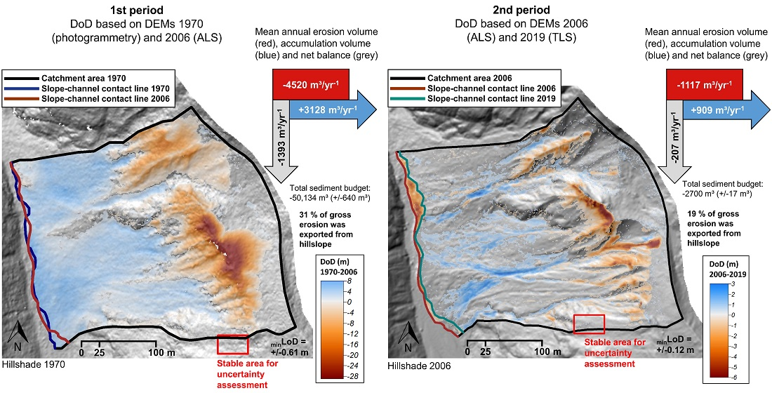
Based on the results of the negative net balances on all test sites in all periods, a strong slope–channel coupling can be stated, but with a clear decrease from the first to the second period. For the test site G1, the export from the gross erosion decreased from 31% to 19%, for G2 from 65% to 46% and for W1 from 61% to 27%. This is consistent with the observations, e.g., of Harvey (2001) [42], that coupling states can change over longer and also shorter time spans after extreme events [21]. This shows that these coupling states can vary greatly in space and time [39,49]. Thus, the existence of functional connectivity, controlled by gravity and water [40] between two sediment cascades [30], the hillslope and the adjacent mountain streams is demonstrated.

Due to the higher runoff of the adjacent proglacial rivers and in combination with heavy precipitation events, the alluvial fans and debris cones were regularly and clearly undercut, especially in the second period. Thus, the formation of terraces and buffering floodplains is strongly influenced, as these are constantly being reworked. [22,47,48]. It can be assumed, that the undercutting of the slope could have an impact on the morphodynamics of the slopes in the sense of a process response system by, e.g., preventing the filling of the gullies and thus levelling or flattening the hillslope channel and slope profiles, as sediments are transferred to the main river. This is in good agreement with the work of Haas (2008) [31], who separated slope and adjacent river in a sediment cascade system, where both systems (slope and river) can influence each other and thus form a process response system.

The headcut of G1 and G2 still shows ongoing high morphodynamics on areas that have been deglaciated at least since 1886/1887 (~132/133 years ago, Figure 1). This ongoing dynamic probably as a consequence of the undercutting of the slopes by the main river stays in contrast to the test sites of, e.g., Curry et al. (2006) [15], where is showed a decreasing dynamic with time and a levelling of the slopes after about 80–140 years. The results of this study show that this seems only to be true for slopes, which are not affected by “external” processes like undercutting by rivers. For the test sites G1 and G2, it can be concluded that the paraglacial adjustment process is still in progress and sediment is still available to the Fagge river, but the dynamics seem to be decreasing. In contrast to G1 and G2, the test site W1 shows a clear increase in morphodynamics. If this is the consequence of the height difference between the G1/2 and W1 test sites (~500 m height difference) or the effect of the large landslide in the second period cannot be clearly stated and must be investigated in future work with a larger sample of test sites.

However, the study also shows that it is difficult to elucidate the nature of the occurring geomorphological processes only by DoD analyses, especially if longer investigation periods are used. To further clarify the nature of the dominant morphogenetic processes, additional investigations are necessary, such as using geophysics (e.g., ground-penetrating radar) to identify different types of sedimentary structures [78,79].

6. Conclusions

The aim of this study was to investigate the morphodynamics on lateral moraines over several decades in proglacial areas and to determine the resulting sediment input from the slopes into the adjacent mountain streams. It can be shown, that the approach of the combination of different remote sensing techniques for the detection of surface changes (historical digital aerial images/photogrammetry and LiDAR) is well suited to cover an investigation period of several decades. Due to the chosen approach of uncertainty assessment for the total sediment budgets as well as the accurately and precisely generated DEMs and the resulting DoDs, the total morphological sediment budgets could be determined very well. Furthermore, the results show that geomorphological processes also can be identified and interpreted using the pattern of the DoD over longer periods. The analyses lead to the following conclusions. The morphodynamics of the hillslopes, as well as the resulting sediment input into the adjacent mountain streams, depend mainly on the characteristics of the slopes (e.g., size, slope length, slope gradient, and elevation) and the resulting higher relief energy on steeper and longer slopes. Individual and rare geomorphological processes of higher magnitudes (e.g., landslides) show a high influence on the mean annual erosion and accumulation volumes by increasing them strongly. Due to the high morphodynamics in the erosion and accumulation areas, vegetation cover is sparse developed and was found mainly in undisturbed areas of the slopes. The three test sites show differences in their morphodynamics. The two test sites on the lateral moraine of the Gepatsch glacier show a decreasing but ongoing high morphodynamics in the upper parts of the slopes. The results show very clear that sediment is still available and the paraglacial adjustment process is still in progress after ~132/133 years since deglaciation. In contrast, the test site on the lateral moraine of the Weißsee glacier shows an increase in morphodynamics. If this is the consequence of differences in height or a consequence of an internal disturbance of the system by the big landslide stays unclear, but it seems that dead ice plays a major role in this case. The test sites are generally subject to changes in external forces, such as an increasing trend in temperature and a decrease in short-term precipitation events (15-min/1 h) but an increase in daily precipitation sum. In particular, with the decreasing trend of precipitation, a correlation with the decrease of morphodynamics can be assumed. Furthermore, the increase in temperature leads to an increase in the runoff of the mountain streams directly adjacent to the slopes due to the higher proportion of meltwater, which in turn has led to a strong undercutting of the slopes in the recent years. In general, there is a strong geomorphic coupling of the investigated test sites, but also a decrease in the efficiency of sediment transport on the slopes into the channels. Thus, the investigated test sites are subject to strong changes of external forces as well as system-internal dynamics.

References

1. Deline, P.; Gruber, S.; Delaloye, R.; Fischer, L.; Geertsema, M.; Giardino, M.; Hasler, A.; Kirkbride, M.; Krautblatter, M.; Magnin, F.; et al. Ice Loss and Slope Stability in High-Mountain Regions. In Snow and Ice-Related Hazards, Risks, and Disasters; Haeberli, W., Whiteman, C., Shroder, J.F., Eds.; Elsevier: Amsterdam, The Netherlands, 2015; pp. 521–561. ISBN 9780123948496. [Google Scholar]
2. Heckmann, T.; Morche, D. (Eds.) Geomorphology of Proglacial Systems. In Landform and Sediment Dynamics in Recently Deglaciated Alpine Landscapes; Springer International Publishing: Cham, Switzerland, 2019; ISBN 9783319941844. [Google Scholar]
3. Haeberli, W.; Beniston, M. Climate Change and Its Impacts on Glaciers and Permafrost in the Alps. Ambio 1998, 27, 258–265. [Google Scholar]
4. Beniston, M. Mountain Climates and Climatic Change: An Overview of Processes Focusing on the European Alps. Pure Appl. Geophys. 2005, 162, 1587–1606. [Google Scholar] [CrossRef] [Green Version]
5. Abermann, J.; Lambrecht, A.; Fischer, A.; Kuhn, M. Quantifying changes and trends in glacier area and volume in the Austrian Ötztal Alps (1969–1997–2006). Cryosphere 2009, 3, 205–2015. [Google Scholar] [CrossRef] [Green Version]
6. Zemp, M.; Hoelzle, M.; Haeberli, W. Six decades of glacier mass-balance observations: A review of the worldwide monitoring network. Ann. Glaciol. 2009, 50, 101–111. [Google Scholar] [CrossRef] [Green Version]
7. Kneisel, C.; Kääb, A. Mountain permafrost dynamics within a recently exposed glacier forefield inferred by a combined geomorphological, geophysical and photogrammetrical approach. Earth Surf. Process. Landf. 2007, 32, 1797–1810. [Google Scholar] [CrossRef]
8. Pauli, H.; Gottfried, M.; Grabherr, G. Effects of climate change on the alpine and nival vegetation of the Alps. J. Mt. Ecol. 2003, 7, 9–12. [Google Scholar]
9. Raffl, C.; Erschbamer, B. Comparative vegetation analyses of two transects crossing a characteristic glacier valley in the Central Alps. Phytocoenologia 2004, 34, 225–240. [Google Scholar] [CrossRef]
10. Huss, M.; Farinotti, D.; Bauder, A.; Funk, M. Modelling runoff from highly glacierized alpine drainage basins in a changing climate. Hydrol. Process. 2008, 22, 3888–3902. [Google Scholar] [CrossRef]
11. Pellicciotti, F.; Bauder, A.; Parola, M. Effect of glaciers on streamflow trends in the Swiss Alps. Water Resour. Res. 2010, 46, 1–16. [Google Scholar] [CrossRef] [Green Version]
12. Majone, B.; Villa, F.; Deidda, R.; Bellin, A. Impact of climate change and water use policies on hydropower potential in the south-eastern Alpine region. Sci. Total Environ. 2016, 543, 965–980. [Google Scholar] [CrossRef]
13. Church, M.; Ryder, J.M. Paraglacial Sedimentation: A Consideration of Fluvial Processes Conditioned by Glaciation. Geol. Soc. Am. Bull. 1972, 83, 3059. [Google Scholar] [CrossRef] [Green Version]
14. Ballantyne, C.K. A general model of paraglacial landscape response. Holocene 2002, 12, 371–376. [Google Scholar] [CrossRef]
15. Curry, A.M.; Cleasby, V.; Zukowskyj, P. Paraglacial response of steep, sediment-mantled slopes to post-‘Little Ice Age’ glacier recession in the central Swiss Alps. J. Quat. Sci. 2006, 21, 211–225. [Google Scholar] [CrossRef]
16. Schiefer, E.; Gilbert, R. Reconstructing morphometric change in a proglacial landscape using historical aerial photography and automated DEM generation. Geomorphology 2007, 88, 167–178. [Google Scholar] [CrossRef]
17. Cossart, E.; Fort, M. Sediment release and storage in early deglaciated areas: Towards an application of the exhaustion model from the case of Massif des Écrins (French Alps) since the Little Ice Age. Nor. Geogr. Tidsskr. Nor. J. Geogr. 2008, 62, 115–131. [Google Scholar] [CrossRef]
18. Carrivick, J.L.; Heckmann, T. Short-term geomorphological evolution of proglacial systems. Geomorphology 2017, 287, 3–28. [Google Scholar] [CrossRef] [Green Version]
19. Ballantyne, C.K. Paraglacial landform succession and sediment storage in deglaciated mountain valleys: Theory and approaches to calibration. Z. Geomorphol. Suppl. 2003, 132, 1–18. [Google Scholar]
20. Orwin, J.F.; Smart, C.C. Short-term spatial and temporal patterns of suspended sediment transfer in proglacial channels, small River Glacier, Canada. Hydrol. Process. 2004, 18, 1521–1542. [Google Scholar] [CrossRef]
21. Haas, F.; Heckmann, T.; Hilger, L.; Becht, M. Quantification and Modelling of Debris Flows in the Proglacial Area of the Gepatschferner/Austria using Ground-based LIDAR. In Erosion and Sediment Yields in the Changing Environment: Proceedings of an IAHS International Commission on Continental Erosion Symposium, held at the Institute of Mountain Hazards and Environment, CAS-Chengdu, China, 11–15 October 2012; Collins, L.A., Golosov, V., Horowitz, A.J., Lu, X., Stone, M., Walling, D.E., Zhang, X., Eds.; IAHS Publication: Wallingford, UK, 2012; Volume 356, pp. 293–302. [Google Scholar]
22. Heckmann, T.; Vericat, D. Computing spatially distributed sediment delivery ratios: Inferring functional sediment connectivity from repeat high-resolution digital elevation models. Earth Surf. Process. Landf. 2018, 43, 1547–1554. [Google Scholar] [CrossRef]
23. Dusik, J. Die aktuelle Geomorphodynamik auf Proglazialen Moränen im Hinteren Kaunertal: Hochaufgelöste Messung und Modellierung der Prozessdynamik Hinsichtlich ihrer Lokalen und Temporalen Variabilität. Ph.D. Thesis, Catholic University of Eichstätt-Ingolstadt, Eichstätt, Germany, 2019. [Google Scholar]
24. Dusik, J.-M.; Neugirg, F.; Haas, F. Slope Wash, Gully Erosion and Debris Flows on Lateral Moraines in the Upper Kaunertal, Austria. In Geomorphology of Proglacial Systems: Landform and Sediment Dynamics in Recently Deglaciated Alpine Landscapes; Heckmann, T., Morche, D., Eds.; Springer International Publishing: Cham, Switzerland, 2019; pp. 177–196. ISBN 9783319941844. [Google Scholar]
25. Tschada, H.; Hofer, B. Total solids load from the catchment area of the Kaunertal hydroelectric power station: The results of 25 years of operation. IAHS Publ. 1990, 194, 121–128. [Google Scholar]
26. Hilger, L. Quantification and Regionalization of Geomorphic Processes using Spatial Models and High-Resolution Topographic Data: A Sediment Budget of the Upper Kauner Valley, Ötztal Alps. Ph.D. Thesis, Catholic University of Eichstätt-Ingolstadt, Eichstätt, Germany, 2017. [Google Scholar]
27. Chorley, R.J.; Kennedy, B.A. Physical Geography. A System Approach; Prentice Hall: London, UK, 1971. [Google Scholar]
28. Caine, N.; Swanson, F. Geomorphic coupling of hillslope and channel systems in two small mountain basins. Zeitschrift für Geomorphologie 1989, 33, 189–203. [Google Scholar]
29. Church, M.; Slaymaker, O. Disequilibrium of Holocene sediment yield in glaciated British Columbia. Nature 1989, 337, 452–454. [Google Scholar] [CrossRef]
30. Burt, T.P.; Allison, R.J. Sediment Cascades. An Integrated Approach; John Wiley & Sons Ltd: Chichester, UK, 2010. [Google Scholar]
31. Haas, F. Fluviale Hangprozesse in Alpinen Einzugsgebieten der Nördlichen Kalkalpen: Quantifizierung und Modellierungsansätze. Ph.D. Thesis, Catholic University of Eichstätt-Ingolstadt, Eichstätt, Germany, 2008. [Google Scholar]
32. Becht, M. Untersuchungen zur Aktuellen Reliefentwicklung in Alpinen Einzugsgebieten; Geobuch Verlag: München, Germany, 1995. [Google Scholar]
33. Heckmann, T.; Haas, F.; Morche, D.; Schmidt, K.-H.; Rohn, J.; Moser, M.; Leopold, M.; Kuhn, M.; Briese, C.; Pfeifer, N.; et al. Investigating an Alpine proglacial sediment budget using field measurements, airborne and terrestrial LiDAR data. In Proceedings of the a Symposium held at the Institute of Mountain Hazards and Environment, Chengdu, China, 11–15 October 2012; Collins, A.L., Golosov, V., Horowitz, A.J., Lu, X., Stone, M., Walling, D.E., Zhang, X., Eds.; pp. 438–447. [Google Scholar]
34. Faulkner, H. Connectivity as a crucial determinant of badland morphology and evolution. Geomorphology 2008, 100, 91–103. [Google Scholar] [CrossRef]
35. Heckmann, T.; Schwanghart, W. Geomorphic coupling and sediment connectivity in an alpine catchment—Exploring sediment cascades using graph theory. Geomorphology 2013, 182, 89–103. [Google Scholar] [CrossRef]
36. Hooke, J. Coarse sediment connectivity in river channel systems: A conceptual framework and methodology. Geomorphology 2003, 56, 79–94. [Google Scholar] [CrossRef]
37. Korup, O. Geomorphic imprint of landslides on alpine river systems, southwest New Zealand. Earth Surf. Process. Landf. 2005, 30, 783–800. [Google Scholar] [CrossRef]
38. Brierley, G.; Fryirs, K.; Jain, V. Landscape connectivity: The geographic basis of geomorphic applications. Area 2006, 38, 165–174. [Google Scholar] [CrossRef]
39. Fryirs, K. (Dis)Connectivity in catchment sediment cascades: A fresh look at the sediment delivery problem. Earth Surf. Process. Landf. 2013, 38, 30–46. [Google Scholar] [CrossRef]
40. Bracken, L.J.; Turnbull, L.; Wainwright, J.; Bogaart, P. Sediment connectivity: A framework for understanding sediment transfer at multiple scales. Earth Surf. Process. Landf. 2015, 40, 177–188. [Google Scholar] [CrossRef] [Green Version]
41. Wohl, E.; Magilligan, F.J.; Rathburn, S.L. Introduction to the special issue: Connectivity in Geomorphology. Geomorphology 2017, 277, 1–5. [Google Scholar] [CrossRef] [Green Version]
42. Harvey, A.M. Coupling between hillslopes and channels in upland fluvial systems: Implications for landscape sensitivity, illustrated from the Howgill Fells, northwest England. CATENA 2001, 42, 225–250. [Google Scholar] [CrossRef]
43. Savi, S.; Schneuwly-Bollschweiler, M.; Bommer-Denns, B.; Stoffel, M.; Schlunegger, F. Geomorphic coupling between hillslopes and channels in the Swiss Alps. Earth Surf. Process. Landf. 2013, 38, 959–969. [Google Scholar] [CrossRef]
44. Kummert, M.; Delaloye, R. Regional-scale inventory of periglacial moving landforms connected to the torrential network system. Geogr. Helv. 2018, 73, 357–371. [Google Scholar] [CrossRef] [Green Version]
45. Fryirs, K.A.; Brierley, G.J.; Preston, N.J.; Spencer, J. Catchment-scale (dis)connectivity in sediment flux in the upper Hunter catchment, New South Wales, Australia. Geomorphology 2007, 84, 297–316. [Google Scholar] [CrossRef]
46. Morche, D.; Schmidt, K.; Heckmann, T.; Haas, F. Hydrology and geomorphic effects of a high-magnitude flood in an alpine river. Geogr. Ann. Ser. A Phys. Geogr. 2007, 89, 5–19. [Google Scholar] [CrossRef]
47. Morche, D.; Haas, F.; Baewert, H.; Heckmann, T.; Schmidt, K.-H.; Becht, M. Sediment transport in the proglacial Fagge River (Kaunertal/Austria). IAHS-AISH Publ. 2012, 356, 72–80. [Google Scholar]
48. Baewert, H.; Morche, D. Coarse sediment dynamics in a proglacial fluvial system (Fagge River, Tyrol). Geomorphology 2014, 218, 88–97. [Google Scholar] [CrossRef]
49. Harvey, A.M. Effective timescales of coupling within fluvial systems. Geomorphology 2002, 44, 175–201. [Google Scholar] [CrossRef]
50. Turnbull, L.; Wainwright, J.; Brazier, R.E. Changes in hydrology and erosion over a transition from grassland to shrubland. Hydrol. Process. 2009, 24, 393–414. [Google Scholar] [CrossRef] [Green Version]
51. Wainwright, J.; Turnbull, L.; Ibrahim, T.G.; Lexartza-Artza, I.; Thornton, S.F.; Brazier, R.E. Linking environmental régimes, space and time: Interpretations of structural and functional connectivity. Geomorphology 2011, 126, 387–404. [Google Scholar] [CrossRef]
52. Heckmann, T.; Cavalli, M.; Cerdan, O.; Foerster, S.; Javaux, M.; Lode, E.; Smetanová, A.; Vericat, D.; Brardinoni, F. Indices of sediment connectivity: Opportunities, challenges and limitations. Earth-Sci. Rev. 2018, 187, 77–108. [Google Scholar] [CrossRef] [Green Version]
53. Gärtner-Roer, I.; Bast, A. (Ground) Ice in the Proglacial Zone. In Geomorphology of Proglacial Systems: Landform and Sediment Dynamics in Recently Deglaciated Alpine Landscapes; Heckmann, T., Morche, D., Eds.; Springer International Publishing: Cham, Switzerland, 2019; pp. 85–98. ISBN 9783319941820. [Google Scholar]
54. Carrivick, J.L.; Geilhausen, M.; Warburton, J.; Dickson, N.E.; Carver, S.J.; Evans, A.J.; Brown, L.E. Contemporary geomorphological activity throughout the proglacial area of an alpine catchment. Geomorphology 2013, 188, 83–95. [Google Scholar] [CrossRef] [Green Version]
55. Betz, S.; Croce, V.; Becht, M. Investigating morphodynamics on Little Ice Age lateral moraines in the Italian Alps using archival aerial photogrammetry and airborne LiDAR data. Z. Geomorphol. 2019, 62, 231–247. [Google Scholar] [CrossRef]
56. Kamleitner, S.M. Is There Still Dead Ice in the Little Ice Age Lateral Moraine? Master’s Thesis, Universität Wien, Vienna, Austria, 2017. [Google Scholar]
57. Eichel, J.; Draebing, D.; Meyer, N. From active to stable: Paraglacial transition of Alpine lateral moraine slopes. Land Degrad. Dev. 2018, 29, 4158–4172. [Google Scholar] [CrossRef]
58. Guzzetti, F.; Peruccacci, S.; Rossi, M.; Stark, C.P. The rainfall intensity–duration control of shallow landslides and debris flows: An update. Landslides 2008, 5, 3–17. [Google Scholar] [CrossRef]
59. Theule, J.I.; Liébault, F.; Loye, A.; Laigle, D.; Jaboyedoff, M. Sediment budget monitoring of debris-flow and bedload transport in the Manival Torrent, SE France. Nat. Hazards Earth Syst. Sci. 2012, 12, 731–749. [Google Scholar] [CrossRef] [Green Version]
60. Baily, B.; Collier, P.; Farres, P.; Inkpen, R.; Pearson, A. Comparative assessment of analytical and digital photogrammetric methods in the construction of DEMs of geomorphological forms. Earth Surf. Process. Landf. 2003, 28, 307–320. [Google Scholar] [CrossRef]
61. Midgley, N.G.; Tonkin, T.N. Reconstruction of former glacier surface topography from archive oblique aerial images. Geomorphology 2017, 282, 18–26. [Google Scholar] [CrossRef] [Green Version]
62. Stark, M.; Neugirg, F.; Kaiser, A.; Della Seta, M.; Schmidt, J.; Becht, M.; Haas, F. Calanchi badlands reconstructions and long-term change detection analysis from historical aerial and UAS image processing. J. Geomorphol. 2020. [Google Scholar] [CrossRef]
63. Heritage, G.; Hetherington, D. Towards a protocol for laser scanning in fluvial geomorphology. Earth Surf. Process. Landf. 2007, 32, 66–74. [Google Scholar] [CrossRef]
64. Scheidl, C.; Rickenmann, D.; Chiari, M. The use of airborne LiDAR data for the analysis of debris flow events in Switzerland. Nat. Hazards Earth Syst. Sci. 2008, 8, 1113–1127. [Google Scholar] [CrossRef] [Green Version]
65. Höfle, B.; Rutzinger, M. Topographic airborne LiDAR in geomorphology: A technological perspective. Z. Geomorphol. Suppl. Issues 2011, 55, 1–29. [Google Scholar] [CrossRef]
66. Williams, R.D.; Rennie, C.D.; Brasington, J.; Hicks, D.M.; Vericat, D. Linking the spatial distribution of bed load transport to morphological change during high-flow events in a shallow braided river. J. Geophys. Res. Earth Surf. 2015, 120, 604–622. [Google Scholar] [CrossRef] [Green Version]
67. Brasington, J.; Rumsby, B.T.; McVey, R.A. Monitoring and modelling morphological change in a braided gravel-bed river using high resolution GPS-based survey. Earth Surf. Process. Landf. 2000, 25, 973–990. [Google Scholar] [CrossRef]
68. Lane, S.N. The Measurement of River Channel Morphology Using Digital Photogrammetry. Photogramm. Rec. 2000, 16, 937–961. [Google Scholar] [CrossRef]
69. Fuller, I.C.; Large, A.R.G.; Charlton, M.E.; Heritage, G.L.; Milan, D.J. Reach-scale sediment transfers: An evaluation of two morphological budgeting approaches. Earth Surf. Process. Landf. 2003, 28, 889–903. [Google Scholar] [CrossRef] [Green Version]
70. Gaeuman, D.A.; Schmidt, J.C.; Wilcock, P.R. Evaluation of in-channel gravel storage with morphology-based gravel budgets developed from planimetric data. J. Geophys. Res. Earth Surf. 2003, 108, 1–16. [Google Scholar] [CrossRef]
71. Rickenmann, D.; Hunzinger, L.; Koschni, A. Flood Events and Sediment Transport during the Rainstorm of August 2005 in Switzerland. Interpraevent 2008 Conf. Proc. 2008, 1, 465–476. [Google Scholar]
72. Vericat, D.; Wheaton, J.M.; Brasington, J. Revisiting the Morphological Approach. In Gravel-Bed Rivers: Processes and Disasters, 1st ed.; Tsutsumi, D., Laronne, J.B., Eds.; John Wiley & Sons: Chichester, UK; Hoboken, NJ, USA, 2017; pp. 121–158. ISBN 9781118971437. [Google Scholar]
73. Rapp, A. Recent Development of Mountain Slopes in Kärkevagge and Surroundings, Northern Scandinavia. Geogr. Ann. 1960, 42, 65–200. [Google Scholar] [CrossRef]
74. Reid, L.M.; Dunne, T. Rapid Evaluation of Sediment Budgets; Catena: Reiskirchen, Germany, 1996. [Google Scholar]
75. Bimböse, M.; Schmidt, K.-H.; Morche, D. High resolution quantification of slope–channel coupling in an alpine geosystem. IAHS Publ. 2010, 337, 300–307. [Google Scholar]
76. Bimböse, M.; Nicolay, A.; Bryk, A.; Schmidt, K.-H.; Morche, D. Investigations on intra- and interannual coarse sediment dynamics in a high-mountain river. Z. Geomorphol. Suppl. Issues 2011, 55, 67–81. [Google Scholar] [CrossRef]
77. Bremer, M.; Sass, O. Combining airborne and terrestrial laser scanning for quantifying erosion and deposition by a debris flow event. Geomorphology 2012, 138, 49–60. [Google Scholar] [CrossRef]
78. Sass, O.; Krautblatter, M. Debris flow-dominated and rockfall-dominated talus slopes: Genetic models derived from GPR measurements. Geomorphology 2007, 86, 176–192. [Google Scholar] [CrossRef]
79. Onaca, A.; Ardelean, A.C.; Urdea, P.; Ardelean, F.; Sărășan, A. Genetic typologies of talus deposits derived from GPR measurements in the alpine environment of the Făgăraș Mountains. Carpathian J. Earth Environ. Sci. 2016, 11, 609–616. [Google Scholar]
80. Warburton, J. An Alpine Proglacial Fluvial Sediment Budget. Geogr. Ann. Ser. A Phys. Geogr. 1990, 72, 261–272. [Google Scholar] [CrossRef]
81. Slaymaker, O. The sediment budget as conceptual framework and management tool. In The Interactions between Sediments and Water. Developments in Hydrobiology; Kronvang, B., Ed.; Springer: Dordrecht, The Netherlands, 2003. [Google Scholar]
82. Tollmann, A. Geologie von Österreich. Die Zentralalpen; Deuticke: Vienna, Austria, 1977. [Google Scholar]
83. Geological Survey of Austria. Geological Map of Austria, 1:2,000,000; Geological Survey of Austria: Vienna, Austria, 1999.
84. Vehling, L. Gravitative Massenbewegungen an Alpinen Felshängen: Quantitative Bedeutung in der Sedimentkaskade Proglazialer Geosysteme (Kaunertal, Tirol). Ph.D. Thesis, Friedrich-Alexander-Universität Erlangen-Nürnberg, Erlangen, Germany, 2016. [Google Scholar]
85. Buckel, J.; Otto, J.-C. The Austrian Glacier Inventory GI 4 (2015) in ArcGis (shapefile) format, supplement to: Buckel, Johannes; Otto, Jan-Christoph; Prasicek, Günther; Keuschnig, Markus (2018): Glacial lakes in Austria—Distribution and formation since the Little Ice Age. Glob. Planet. Chang. 2018, 164, 39–51. [Google Scholar] [CrossRef]
86. Nicolussi, K.; Patzelt, G. Untersuchungen zur holozänen Gletscherentwicklung von Pasterze und Gepatschferner (Ostalpen). Z. Gletsch. Glazialgeol. 2001, 36, 1–87. [Google Scholar]
87. Sonklar, K. Die Oetzthaler Gebirgsgruppe, mit Besonderer Rücksicht auf Orographie und Gletscherkunde; Justus Perthes: Gotha, Germany, 1861. [Google Scholar]
88. Finsterwalder, S.; Schunk, H.; Blümcke, A. Die Zunge des Gepatschferners 1886/87; Stich u. Druck: Kartogr. Inst. v. H. Petters: Hildburghausen, Germany, 1888. [Google Scholar]
89. Finsterwalder, S. Der Talschluss des Kaunertals in den Ötztaler alpen mit dem Gepatsch- und Weißseeferner; 1928. [Google Scholar]
90. Veit, H. Die Alpen. Geoökologie und Landschaftsentwicklung; Ulmer: Stuttgart, Germany, 2002. [Google Scholar]
91. Brunner, K. Maps of Gepatschferner—The Tongue, Austria. In WGMS (1988): Fluctuations of Glaciers 1980–1985; Haeberli, W., Müller, P., Eds.; IAHS (ICSI)/UNEP/UNESCO; World Glacier Monitoring Service: Zurich, Switzerland, 1988; Volume 5. [Google Scholar]
92. Henninger, R. Veränderungen der Zungenlage des Gepatschferners seit 1886/87. Ph.D. Thesis, Fachhochschule Karlsruhe, Karlsruhe, Germany, 1985. [Google Scholar]
93. Brunner, K. Maps of Gepatschferner—Tongue Position, Austria. In WGMS (1988): Fluctuations of Glaciers 1980–1985; Haeberli, W., Müller, P., Eds.; IAHS (ICSI)/UNEP/UNESCO; World Glacier Monitoring Service: Zurich, Switzerland, 1988; Volume 5. [Google Scholar]
94. ÖAV; DAV. Ötztaler Alpen. Blatt Weisskugel-Wildspitze (30/2); Vienna, Austria, 1962. [Google Scholar]
95. Army Map Service. Weisskugel Sheet 172/1-4, 1st ed.; Army Map Service: Washington, DC, USA, 1952.
96. Patzelt, G. The Austrian Glacier Inventory GI 1, 1969, in ArcGIS (Shapefile) Format; 2015. [Google Scholar]
97. Wild Heerbrugg AG. Calibration Certificate Wild Camera No. 21 At. 109; 1968. [Google Scholar]
98. Wild Heerbrugg AG. Calibration Certificate Wild Camera No. 21 At. 7; 1969. [Google Scholar]
99. Gomez, C.; Hayakawa, Y.; Obanawa, H. A study of Japanese landscapes using structure from motion derived DSMs and DEMs based on historical aerial photographs: New opportunities for vegetation monitoring and diachronic geomorphology. Geomorphology 2015, 242, 11–20. [Google Scholar] [CrossRef] [Green Version]
100. Glira, P.; Pfeifer, N.; Briese, C.; Ressl, C. A Correspondence Framework for ALS Strip Adjustments based on Variants of the ICP Algorithm. Photogramm. Fernerkund. Geoinf. 2015, 275–289. [Google Scholar] [CrossRef]
101. Agisoft Metashape. In 1970—Processing Report 30 April 2020; Internal Document, Unpublished; Eichstätt, Germany, 2020.
102. Agisoft Metashape. In 1971—Processing Report 30 April 2020; Internal Document, Unpublished; Eichstätt, Germany, 2020.
103. RIEGL Laser Measurement Systems GmbH. Data Sheet, RIEGL VZ-4000; RIEGL Laser Measurement Systems GmbH: Horn, Austria, 2019. [Google Scholar]
104. O’Callaghan, J.F.; Mark, D.M. The extraction of drainage networks from digital elevation data. Computer vision, graphics, and image processing. Comput. Vis. Graph. Image Process. 1984, 28, 323–344. [Google Scholar]
105. Lane, S.N.; Westaway, R.M.; Murray Hicks, D. Estimation of erosion and deposition volumes in a large, gravel-bed, braided river using synoptic remote sensing. Earth Surf. Process. Landf. 2003, 28, 249–271. [Google Scholar] [CrossRef]
106. Milan, D.J.; Heritage, G.L.; Large, A.R.G.; Fuller, I.C. Filtering spatial error from DEMs: Implications for morphological change estimation. Geomorphology 2011, 125, 160–171. [Google Scholar] [CrossRef]
107. Hodgson, M.E.; Bresnahan, P. Accuracy of Airborne Lidar-Derived Elevation. Photogramm. Eng. Remote Sens. 2004, 70, 331–339. [Google Scholar] [CrossRef] [Green Version]
108. Abellán, A.; Oppikofer, T.; Jaboyedoff, M.; Rosser, N.J.; Lim, M.; Lato, M.J. Terrestrial laser scanning of rock slope instabilities. Earth Surf. Process. Landf. 2014, 39, 80–97. [Google Scholar] [CrossRef]
109. Fan, L.; Atkinson, P.A. Accuracy of Digital Elevation Models Derived From Terrestrial Laser Scanning Data. IEEE Geosci. Remote Sens. Lett. 2015, 12, 1923–1927. [Google Scholar] [CrossRef]
110. Bakker, M.; Lane, S.N. Archival photogrammetric analysis of river-floodplain systems using Structure from Motion (SfM) methods. Earth Surf. Process. Landf. 2017, 42, 1274–1286. [Google Scholar] [CrossRef] [Green Version]
111. Westaway, R.M.; Lane, S.N.; Hicks, D.M. The development of an automated correction procedure for digital photogrammetry for the study of wide, shallow, gravel-bed rivers. Earth Surf. Process. Landf. 2000, 25, 209–226. [Google Scholar] [CrossRef]
112. Micheletti, N.; Chandler, J.H.; Lane, S.N. Investigating the geomorphological potential of freely available and accessible structure-from-motion photogrammetry using a smartphone. Earth Surf. Process. Landf. 2015, 40, 473–486. [Google Scholar] [CrossRef] [Green Version]
113. Smith, M.W.; Vericat, D. From experimental plots to experimental landscapes: Topography, erosion and deposition in sub-humid badlands from Structure-from-Motion photogrammetry. Earth Surf. Process. Landf. 2015, 40, 1656–1671. [Google Scholar] [CrossRef] [Green Version]
114. Anderson, S.W. Uncertainty in quantitative analyses of topographic change: Error propagation and the role of thresholding. Earth Surf. Process. Landf. 2019, 44, 1015–1033. [Google Scholar] [CrossRef]
Figure 1. Location of the test sites, historical glacier extents, TLS positions, soil pits, vegetation plots, and the meteorological and hydrological measurement stations. The images were taken during the 2019 field campaign on 26 August 2019 (W1/southern direction) and 12 August 2019 (G1 and G2/northeast direction). Sources of the Hillshades: 2017: ALS (Section 3.1) and 2019: TLS (Section 3.1). Sources of the glacier extents: ~1855/End of LIA: Own mapping of the lateral moraines in the field, from orthophotos (e.g., 1953/2015, Section 3.1) and DEMs (e.g., 2017, Section 3.1), 1886/1887: Finsterwalder et al. (1888) [88] in the corresponding map of Brunner (1988) [91], 1922: Finsterwalder (1928) [89], 1940: Henninger (1985) [92] in the corresponding map of Brunner (1988) [93], 1942/1943: ÖAV and DAV (1962) [94], 1945: Army Map Service (1952) [95], 1953: Orthophoto (BEV, Section 3.1), 1969: Patzelt (2015) [96], and 2015: Buckel and Otto (2018) [85].
Water 12 03375 g001
Figure 2. Overview of the historical images and the extracted ground control points (GCP), Source: Basemap ArcGis, Esri.
Water 12 03375 g002
Figure 3. Light detection and ranging (LiDAR) point cloud acquisition of the test sites (G1/G2) using the TLS VZ-4000 (25 June 2019).
Water 12 03375 g003
Figure 4. DEMs of difference (DoD) error estimation, determined using stable areas on or close to the test sites (Figure 5).
Water 12 03375 g004
Figure 5. DoDs of all test sites in the corresponding periods with the determined morphological sediment budgets, mean annual erosion volume (red), mean annual deposition volume (blue), and the mean annual resulting net balance (grey) (m3). The DoDs of the first period are projected on the Hillshade of 1970/1971 and the DoDs of the second period on the Hillshade of 2006 (accordingly also the contour lines), each with a 40% transparency. The uncertainty of the total net balance and the minimum Level of Detection (minLoD) is based on the six stable areas (red rectangles) at or near the test sites. The corresponding approaches used are described in Section 3.2.2.
Water 12 03375 g005
Figure 6. Mean annual erosion volume (red), mean annual deposition volume (blue) and the respective net balance in the corresponding periods (a) 1970/1971–2006 (first period) and (b) 2006–2019 (second period).
Water 12 03375 g006
Figure 7. Mapping of the land cover classes. The mapping of the vegetation types was based on an orthophoto from 2015 (Section 3.1 and Section 3.3.1) and field surveys in 2020. The vegetation mapping is projected on the hillshade of the ALS dataset 2017.
Water 12 03375 g007
Figure 8. Mean annual sediment input (t) from the slopes into the channels in (a) the first period and (b) the second period. In addition, the change of the sediment input (%) from the second compared to the first period is demonstrated.
Water 12 03375 g008
Figure 9. Precipitation measured at the weather stations: (a) DF (32 years), (b) GA (10 years), and (c) WS (13 years). The blue vertical line (a) marks the 5 September 2006 (ALS recording of the topography of the test sites and separation of the two periods).
Water 12 03375 g009
Figure 10. Time series analysis of gauging station GA: (a) Maximum hourly runoff (m3/s) of each year and trend analysis (1977–2019) and (b) mean hourly runoff events of the respective months (1977–2019). The blue vertical line (a) marks the 5 September 2006 (ALS recording of the topography of the test sites and separation of the two periods).
Water 12 03375 g010