The Role of Hydrological Signatures in Calibration of Conceptual Hydrological Model

Abstract

Determining an optimal calibration strategy for hydrological models is essential for a robust and accurate water balance assessment, in particular, for catchments with limited observed data. In the present study, the hydrological model Bilan was used to simulate hydrological balance for 20 catchments throughout the Czech Republic during the period 1981–2016. Calibration strategies utilizing observed runoff and estimated soil moisture time series were compared with those using only long-term statistics (signatures) of runoff and soil moisture as well as a combination of signatures and time series. Calibration strategies were evaluated considering the goodness-of-fit, the bias in flow duration curve and runoff signatures and uncertainty of the Bilan model. Results indicate that the expert calibration and calibration with observed runoff time series are, in general, preferred. On the other hand, we show that, in many cases, the extension of the calibration criteria to also include runoff or soil moisture signatures is beneficial, particularly for decreasing the uncertainty in parameters of the hydrological model. Moreover, in many cases, fitting the model with hydrological signatures only provides a comparable fit to that of the calibration strategies employing runoff time series.

1. Introduction

Hydrological models are commonly employed to calculate the hydrological balance of a catchment using various calibration strategies (i.e., diverse objective criteria including various variables, different optimization algorithms, etc.). The applied calibration strategy affects the performance of the hydrological model. The widely used manual (expert) calibration of parameters is strongly influenced by the experience of the hydrologist; it is time-consuming and strongly affects the quality of the calibrated model [1]. The automatic calibration, on the other hand, is fast and the performance of the model simulations are explicitly linked to the parameter values within the optimization criteria. The automatic calibration of hydrological models typically uses observed runoff time-series to optimize the parameters. This is, however, not possible in catchments with limited observations, especially if gauged stations are not available. In addition, due to equifinality, models of similar (good) performance may result from models with very different parameter sets and therefore not simulate the physical processes properly.

In ungauged catchments, the water balance can be estimated using different methods, e.g., extrapolation of hydrological model parameters [2], the spatial proximity [3], estimation of the spatially distributed variables from soils and other geo-spatial datasets [4], the physical similarity [5], scaling relationships [6], regression-based methods [7], the hydrological similarity [8] and employing the runoff signatures (indices characterizing hydrologic behavior, [9]). The methods utilising hydrological signatures can be further divided, according to the prediction methods, into hydrological modelling based methods [10,11], and multiple regression methods [12,13] including data-driven methods such as genetic programming [14,15] and hydrological similarity based approaches [16].

Recently, a number of studies pointed out that relying solely on calibration of hydrological models with respect to observed runoff may result in inappropriate representation of hydrological processes and highlighted the importance of expert knowledge [17,18] and/or multi-objective calibration [19].

One approach to constrain the calibration of the hydrological model is to consider hydrological signatures (typically some long-term statistics of runoff, soil moisture, snow regime). They are derived from observed or simulated time series [20] with a purpose to supplement catchment information [21], to evaluate model performance [22] or to refine calibration techniques [23]. The selection of signatures should consider their identifiability, robustness, consistency, representativeness and discriminatory power [20].

Different processes contributing to resulting hydrograph can be also accounted for by the segmentation of the flow duration curve (FDC) within calibration of the hydrological model [4,24]. For instance, it has been shown that fair balance between very high and very low flows can be achieved using five segments of the FDC (Q2–Q5, Q5–Q20, Q20–Q70, Q70–Q95, Q95) and evaluating the performance for each segment and combining it into single objective function [25].

In this paper, we explore the role of hydrological signatures within calibration of the hydrological model. Specifically, we like to answer following questions: To what extent do hydrological signatures improve calibration of conceptual hydrological model? Is calibration of conceptual hydrological model possible considering hydrological signatures only? A hydrological model Bilan is used to determine the hydrological balance for 20 gauged catchments in the Czech Republic utilizing four different calibration strategies: (1) expert calibration, (2) standard automatic calibration, (3) the standard automatic calibration considering hydrological signatures together with runoff and soil moisture time series, and (4) hydrological signatures only. The objectives of this study are to (i) evaluate the performance of different calibration strategies, (ii) assess the added value of hydrological signatures and soil moisture estimates, and (iii) determine to what extent are the time series data necessary when modelling hydrological balance.

This paper is structured as follows: Section 2 introduces the area of interest and input data. The hydrological model Bilan, four calibration strategies and model evaluation are described in Section 3. Results and discussion are presented in Section 4 and Section 5 together with a detailed assessment of the calibration strategies with respect to goodness-of-fit (GOF), uncertainty of Bilan model parameters (BP), and runoff signatures (RS). The paper is concluded in Section 5.

2. Study Area and Data

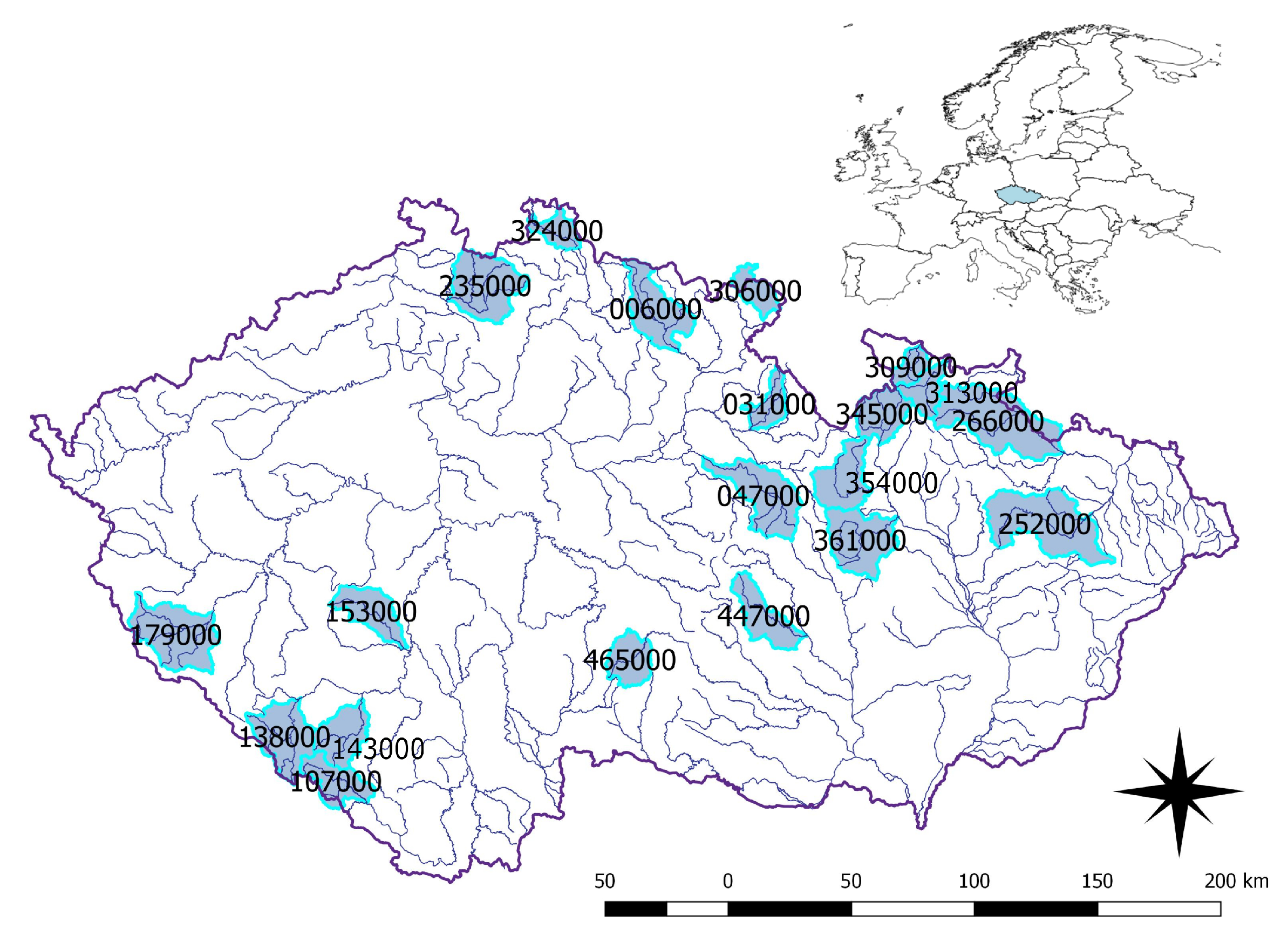
The 20 considered catchments are located in the Czech Republic, where long-term mean precipitation for the 1981–2010 (climatological reference period for Czech Republic) period is 709.5 mm, mean annual temperature is 7.9 °C and mean runoff is 205.5 mm [26]. The selected catchments are shown in Figure 1, with the numbers referring to catchment IDs. The majority of the catchments is located in the northern part of the territory (235000-Ploučnice, 324000-Smědá, 006000-Labe, 306000-Stěnava, 031000-Bělá-Častolovice, 309000-Vidnávka, 313000-Bělá-Mikulovice, 266000-Opava, 354000-Moravská Sázava, the others extend into the central part (047000-Loučná, 361000-Trebůvka, 252000-Odra, 447000-Loučka) and southern part of the territory (179000-Radbuza, 153000-Skalice, 143000-Volyňka, 138000-Otava, 107000-Teplá Vltava). Only catchments with freely available data (in the time of preparation of this study) without significant anthropogenic influence were selected. For selected catchments, mean annual precipitation is 792.5 mm, mean temperature is 7.3 °C, average annual soil water storage is 997.1 mm and mean annual runoff is 318.8 mm. The catchment areas range from 348 to 932 ${\mathrm{km}}^2$, with a mean size of 454 ${\mathrm{km}}^2$.

Monthly time series of temperature (°C), precipitation (mm) and observed runoff (mm) were provided for each catchment by the Czech Hydrometeorological Institute and the soil moisture estimates (mm) by the Global Change Research Institute of the Czech Academy of Sciences. The soil moisture estimates are based on the simulation of the SoilClim model—a model for water balance and the hydric and thermic soil regime assessment [27].

3. Methods

The hydrological model Bilan was used for the assessment of water balance in 20 catchments (Figure 1) considering four calibration strategies: expert calibration, standard automatic calibration, calibration considering runoff and soil moisture time series in combination with hydrological signatures, and calibration with hydrological signatures only. The resulting parameter sets were then evaluated with respect to: (i) goodness-of-fit between observed and simulated runoff (GOF, hydroGOF [28]), (ii) uncertainty of the Bilan model parameters and (BP) (iii) selected runoff and soil moisture signatures (RS). This section introduces the model, the calibrations strategies and the evaluation metrics.

3.1. Bilan Hydrological Model

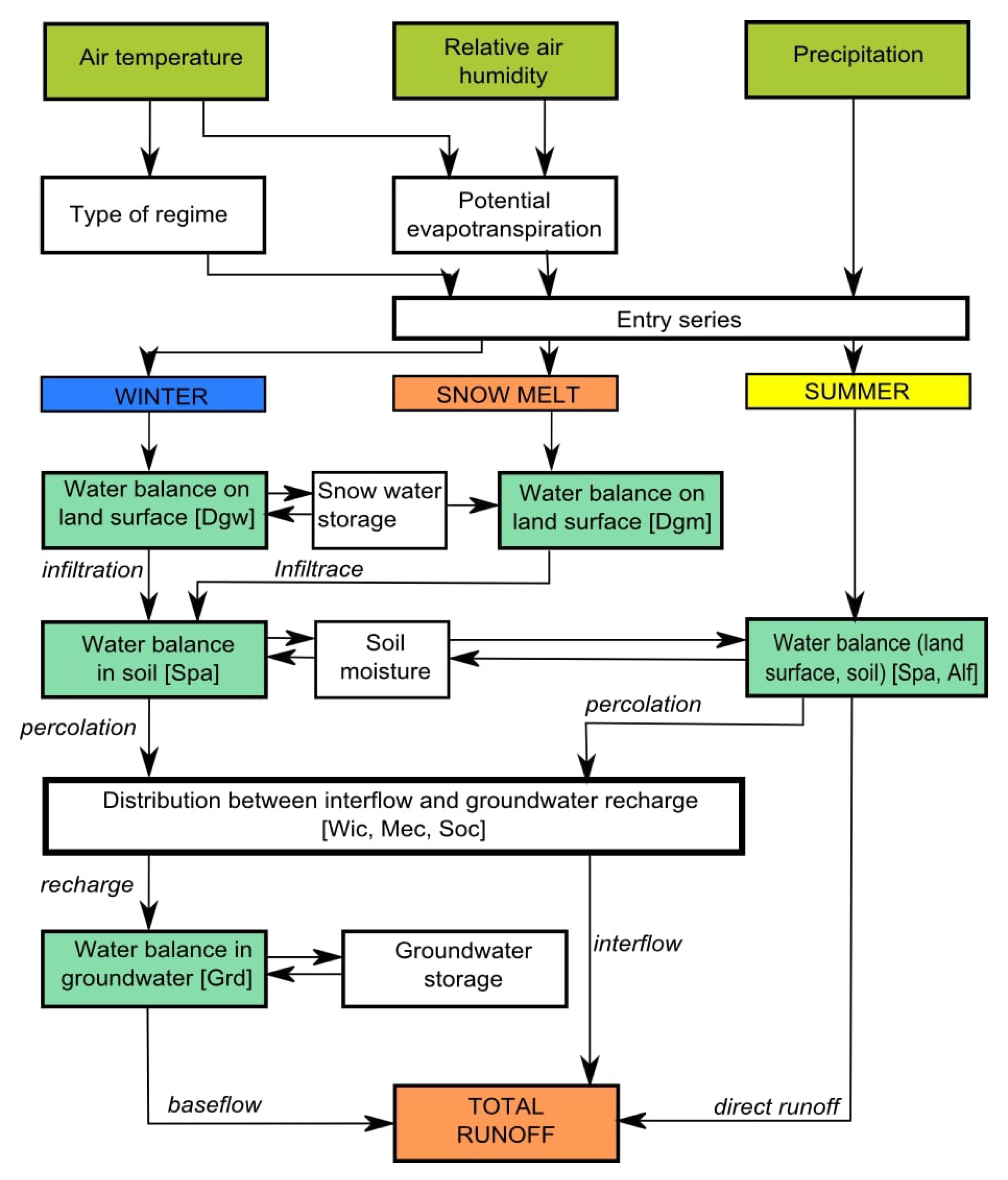
The hydrological model Bilan [29,30] is a conceptual rainfall-runoff model that is used for water balance assessment in the Czech Republic. For partly or fully conceptual models, some parameters cannot be considered as physically measured (or measurable) quantities and thus have to be estimated on the basis of the available data and information [31]. The structure of the model is formed by a number of storage components and a set of their relationships based on basic principles of water balance as well as simple mathematical concepts such as linear reservoir. This structure is similar to a well-known hydrology model HBV (Hydrologiska Byråns Vattenbalansavdelning model) [32]. The water balance in model Bilan is described in three zones: on the ground, in the aeration zone, including vegetation cover, and in the groundwater [33].

The input variables are described in

Table 1. Input and output variables and parameters of the Bilan model.

Input Variables		Units
Variables	Description
P	precipitation	(mm)
R	runoff	(mm)
T	air temperature	(°C)
H	relative air humidity	(%)
PET	potential evapotranspiration	(mm)
TS	optional time series	(mm)
Calculated variables
Fluxes	Description
PET	potential evapotranspiration	(mm)
ET	basin evapotranspiration	(mm)
INF	infiltration into the soil	(mm)
PERC	percolation throught the soil layer	(mm)
I	interflow	(mm)
DR	direct runoff	(mm)
BF	base flow (simulated)	(mm)
RM	total runoff (simulated)	(mm)
State variables	Description
SS	snow water storage	(mm)
SW	soil moisture	(mm)
GS	groundwater storage	(mm)
DS	direct runoff storage	(mm)
DEFV	deficet volumes	(mm)
Model parameters
Parameters	Description
SPA	capacity of soil moisture storage
DGM	temperature and snow melting factor
DGW	water available on the land surface under winter conditions
ALF	controls the proportion of precipitation transformed into the direct runoff
SOC	distribution of percolation into interflow and groundwater recharge under summer cond.
MEC	distribution of percolation into interflow and groundwater recharge under conditions of snow melting
WIC	distribution of percolation into interflow and groundwater recharge under winter cond.
GRD	parameter controlling outflow from groundwater storage (base flow)

, in our case we used the input variable precipitation (P (mm)), air temperature (T (°C)) and optional time-series-soil water (mm)). In the model are individual components divided as input data, water balance component, and resulting parameters. The monthly type used algorithms depend on the condition of the particular month. Used mean monthly temperature as well as in the daily type the model distinguish the winter and summer conditional. In the monthly regime the total runoff ($RM$ (mm)) is calculated as a sum of direct runoff ($DR$), interflow (I), and baseflow ($BS$) [30].

The model is shown in Figure 2 displaying input data, simulated storages and fluxes. See [34,35,36,37] for further details. The parameters of the model are identified (calibrated) using shuffled complex evolution (SCE-UA), Ref. [38] in combination with the differential evolution (DE) method [39]. The algorithm is stochastic and therefore allows for assessment of the uncertainty in the model parameters by repeated calibration. The standard calibration involves minimization of the error in simulated runoff in comparison to observed runoff represented by the value of the selected objective function (OF). However, the model also allows for widening the OF to consider also time series of other variables (typically soil moisture or baseflow estimates) or even individual hydrological signatures such as mean or variance of runoff, indicators of extremes etc.

3.2. Calibration Strategies

The purpose of testing the four calibration strategies was to find such calibration setup that would minimize the bias in simulated water balance and the uncertainty in the estimated model parameters. In addition, while the first three calibration strategies (expert, standard automatic, time series with hydrological signatures) require time series of observed runoff, the fourth (calibration with hydrological signatures) can also be applied at ungauged catchments since the hydrological signatures can often be successfully interpolated from available data or estimated from general formulas.

The available time period (1981–2016) was split into calibration (1981–1998) and validation (1999–2016) period, the former being used for the identification of model parameters and the latter for the evaluation of model performance. Since the stochastic optimization algorithm implemented in the Bilan model allows for the assessment of parameter uncertainty, we fitted the model 15 times for all calibration strategies except for the expert calibration for which only the “best” parameter set was provided.

3.2.1. Expert Calibration

This strategy builds upon knowledge of the catchments and experience with hydrological modelling and is frequently applied in the case of studies for individual catchments over the Czech Republic. Typically, the expert constrains the optimization ranges of model parameters and then runs the optimization procedure. In this perspective, this calibration strategy does not always result in the best possible match between observed and simulated runoff, but at the same time, it ensures that all water balance components have reasonable values and respect physical conditions of the catchments. Therefore throughout the paper, we take these results as a reference. The parameter sets considered here were provided by experts from T. G. Masaryk Water Research Institute (developer of the Bilan model).

3.2.2. Standard Automatic Calibration

The standard automatic calibration, uses differential evolution to minimize the error between time series of observed and simulated runoff. The advantage of the automatic calibration is that it is faster than manual calibration and can be applied over large sets of catchments. It often also results in a better match between observed and simulated runoff than the manual calibration. The downside of the automatic calibration is that for some catchments the simulated water balance (and/or model parameters) may not be realistic resulting in, e.g., excessive ground water or soil water accumulation, unrealistic snow cover, etc.

3.2.3. Calibration with Hydrological Signatures

The last two calibration strategies involve hydrological signatures either in combination with runoff and/or soil moisture time series or as the only component of the objective function (OF). Model calibration was performed in 15 iterations. As the hydrological signatures, we used mean, standard deviation and interquartile range of runoff and soil moisture. The difference between the time series in the OFs was represented by mean percent bias, the match between the hydrological signatures by relative percent difference. The individual components of the OFs were summed to result in a single value. In this paper we considered 52 OFs as given in

Table A1. Optimal OFs are denoted in bold. The time series column contains time series as runoff (R) and soil moisture (SW). The column’s hydrological signature of (R) and (SW) is combined with statistical indicators as mean, IQR, sd and selected settings (*).

ID	Time Series		R-Signatures			SW-Signatures
	R	SW	mean	IQR	sd	mean	IQR	sd
Automatic	*
R-mean			*
R-iqr				*
R-sd					*
SW-mean						*
SW-iqr							*
SW-sd								*
SW-optim		*
R2-mean-sd			*		*
R2-mean-iqr			*	*
R2-mean-optim	*		*
R2-sd-iqr				*	*
R2-sd-optim	*				*
R2-iqr-optim	*			*
SW2-mean-iqr						*	*
SW2-mean-sd						*		*
SW2-mean-optim		*				*
SW2-sd-iqr							*	*
SW2-sd-optim		*						*
SW2-iqr-optim		*					*
RSW-mean-mean			*			*
RSW-mean-sd			*					*
RSW-mean-optim		*	*
RSW-mean-iqr			*				*
RSW-sd-sd					*			*
RSW-sd-optim		*			*
RSW-sd-iqr					*		*
RSW-optim-optim	*	*
RSW-optim-iqr	*						*
RSW-iqr-iqr				*			*
RSW2-mean-mean-sd			*			*		*
RSW2- mean-mean-optim		*	*			*
RSW2-mean-mean-iqr			*			*	*
RSW2-sd-sd-mean					*	*		*
RSW2-sd-sd-optim		*			*			*
RSW2-sd-sd-iqr					*		*	*
RSW2-optim-optim-sd	*	*						*
RSW2-optim-optim-mean	*	*				*
RSW2-optim-optim-iqr	*	*					*
RSW2-iqr-iqr-mean				*		*	*
RSW2-iqr-iqr-sd				*			*	*
RSW2-iqr-iqr-optim		*		*			*
RSW2-mean-sd-optim		*	*					*
RSW2-sd-mean-optim		*	*		*
RSW2-optim-mean-sd	*					*		*
RSW2-iqr-sd-optim		*		*				*
RSW2-sd-iqr-optim		*			*		*
RSW2-optim-iqr-sd	*						*	*
RSW2-iqr-mean-optim		*		*		*
RSW2-mean-iqr-optim		*	*				*
FDC-all	*
FDC-180	*
FDC-300-330-355-364	*

. More than a half of the OFs uses only signatures.

The OFs can be split into six groups:

• Single-component OFs with runoff (R);
• Single-component OFs with soil moisture (SW);
• Two-component OFs with runoff (R2);
• Two-component OFs with soil moisture (SW2);
• Two-component OFs with runoff and soil moisture (RSW);
• Three-component OFs (RSW2).

The specific combinations of variables, time series and signatures is clear from Table A1.

The aim of the introduction of hydrological signatures and/or soil moisture time series is to constrain the uncertainty in model parameters experienced with the automatic calibration and to test whether reasonable runoff simulation can be obtained without observed runoff time series.

3.3. Model Evaluation

The performance of each calibrated parameter set was evaluated with respect to the results of the expert calibration. This means that we like to evaluate to what extent we are able to obtain results close to the expert calibration but with limited information (and without expert knowledge). The parameter sets were evaluated considering:

(a)

Goodness-of-fit expressed (GOF) as the root mean square error (RMSE; [40]) and Kling–Gupta efficiency (KGE; [41]) of the simulated runoff with respect to runoff simulated by the parameter set resulting from the expert calibration (further denoted as the expert simulation).

The RMSE is given by

$$RMSE=\sqrt{(\frac{1}{n})\sum _{i=1}^n{(y_i-x_i)}^2}$$

(1)

where $y_i$ is expert simulation for i-th case, $x_i$ the average of the expert simulation and N is the total number of simulated values. It was used as standard statistical metric, that gives a relatively high weight to large errors.

The KGE is calculated according to

$$KGE=1-\sqrt{{\left(s\left[1\right]\times (r-1)\right)}^2+{\left(s\left[2\right]\times (\alpha -1)\right)}^2+{\left(s\left[3\right]\times (\beta -1)\right)}^2},$$

(2)

where s is numeric weight vector of length 3 (here with all elements equal to 1), which combines the Pearson product-moment correlation coefficient (r), the ratio between the standard deviations ($\alpha$) and the ratio between the mean of the expert simulation and simulation calibrated with particular OF ($\beta$).

(b)

difference in the distribution of Bilan model parameters (BP) Spa (controlling soil depth) and Grd (controlling baseflow) between expert-calibrated parameters (see Section 3.2) and calibration with particular OF.

(c)

relative difference in mean and the 20th (Q20) and 80th (Q80) percentile of runoff and soil moisture from the expert simulation with respect to the same signatures from the simulation calibrated with particular OF.

The relative differences are preferred here over the absolute in order to allow for comparison between catchments. To assess the performance of different calibration strategies, we subsequently ranked the results of individual strategies, according to the criteria above, for each catchment. The calibration strategies with the overall best performance were further evaluated separately as well-denoted selected characteristics.

4. Results and Discussion

This section presents a detailed assessment of the calibration strategies with respect to the flow duration curve, goodness-of-fit (RMSE, KGE), uncertainty of Bilan model parameters (Spa, Grd) and runoff signatures (Q20, Q80), according to different calibration strategies.

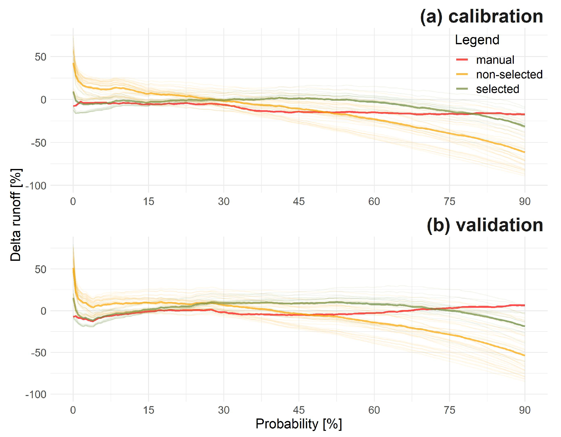
4.1. Runoff Difference Probability Curve

The runoff difference probability curve (Figure 3) was considered for evaluation of calibration, which shows the probability of the relative difference of the modelled runoff and the observation. The low flow are underestimated for selected (95th percentile is −49% of runoff for calibration and −37% for validation) and non-selected (95th percentile is −77% of runoff for calibration and −75% for validation) calibration strategies. The expert calibration results in runoff that matches the observed data closely. For validation, the runoff from expert calibration is positively biased for low flows (95th percentile is 8% of runoff). The selected well-performing calibration strategies are approaching the expert calibration and observed data fairly well.

4.2. Goodness-Of-Fit

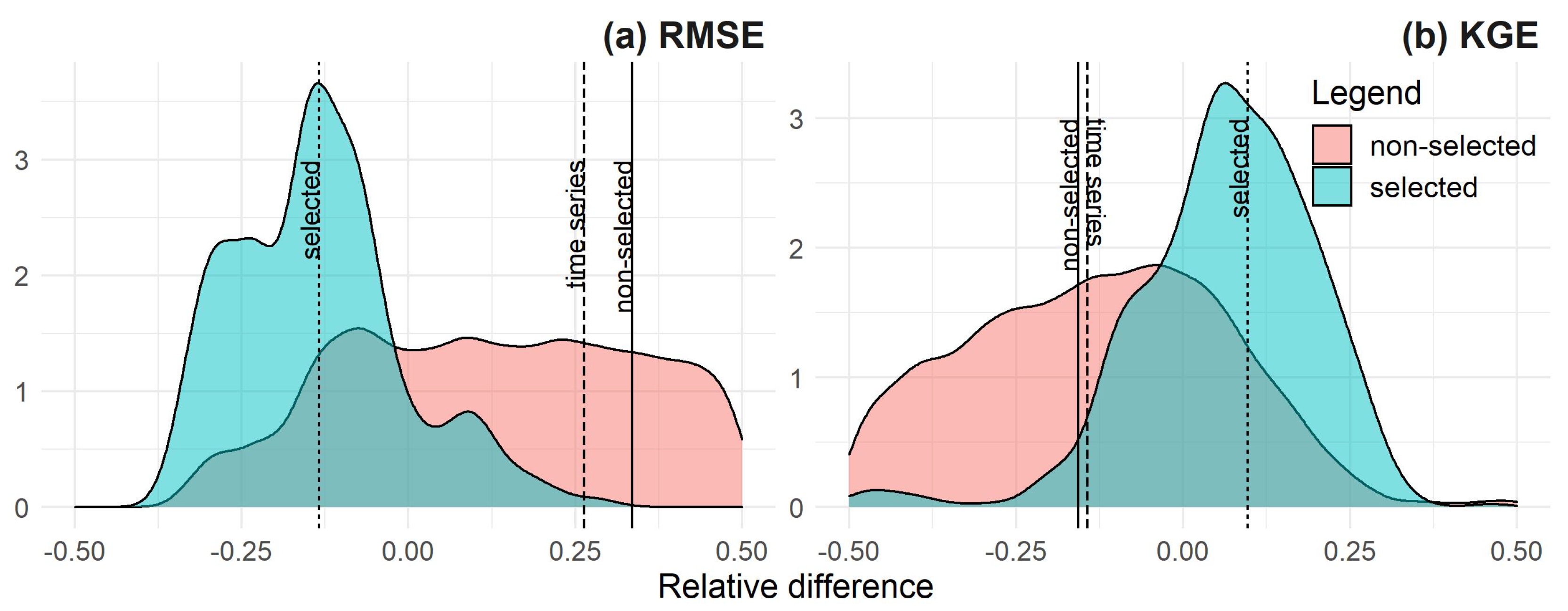
The results for different calibration strategies are compared to those of expert calibration. From the evaluation of goodness-of-fit (GOF), it is obvious that the automatic calibration provides slightly lower RMSE and improves KGE for calibration (RMSE was improved by 0.134 and the KGE by −0.097 on average) with respect to expert calibration.

For validation, the results are not much different. Obviously, introducing runoff and soil moisture signatures has negative impacts on the goodness-of-fit (GOF) metrics. This is logical since a similar metric to RMSE/KGE is used for the automatic calibration, while the calibration criterion for strategies including runoff/soil moisture signatures are more complex. Clearly, the soil moisture signatures alone are not able to provide a reasonable fit. On the other hand, the calibration strategies, including runoff or runoff and soil moisture signatures, performed reasonably for both calibration and validation. It is also obvious that strategies which consider time series data perform better than those based on signatures only. However, the signature-only strategies are also able to provide reasonable results. A quantitative comparison for all groups of objective functions (OFs), with respect to RMSE and KGE, is given in

Table 2. Difference in RMSE (a) and KGE (b) for all groups of objective functions with respect to expert calibration. Automatic, time series + signatures and signatures only mean calibration strategies which combine runoff (R), soil moisture (SW) or runoff + soil moisture (R + SW).

GOF	Automatic		Time Series + Signatures						Signatures Only
			R		SW		R + SW		R		SW		R + SW
	Mean	Median	Mean	Median	Mean	Median	Mean	Median	Mean	Median	Mean	Median	Mean	Median
RMSE	0.134	0.142	0.125	0.138	−0.560	−0.478	−0.257	−0.183	−0.303	−0.222	−0.537	−0.454	−0.383	−0.295
KGE	−0.097	−0.077	−0.099	−0.080	0.270	0.265	0.151	0.129	0.098	0.107	0.236	0.232	0.170	0.156

.

We further compared the distribution of differences in validation of RMSE and KGE between the selected (best-performing) objective functions (OFs) and the rest (Figure 4). It is obvious that the selected OFs provide consistent improvement in both RMSE and KGE, while the rest of the OFs are often worsening the results. In addition, taking into an account the time-series-based OFs only (without signatures) leads to considerably worse results.

4.3. Uncertainty of Bilan Model Parameters

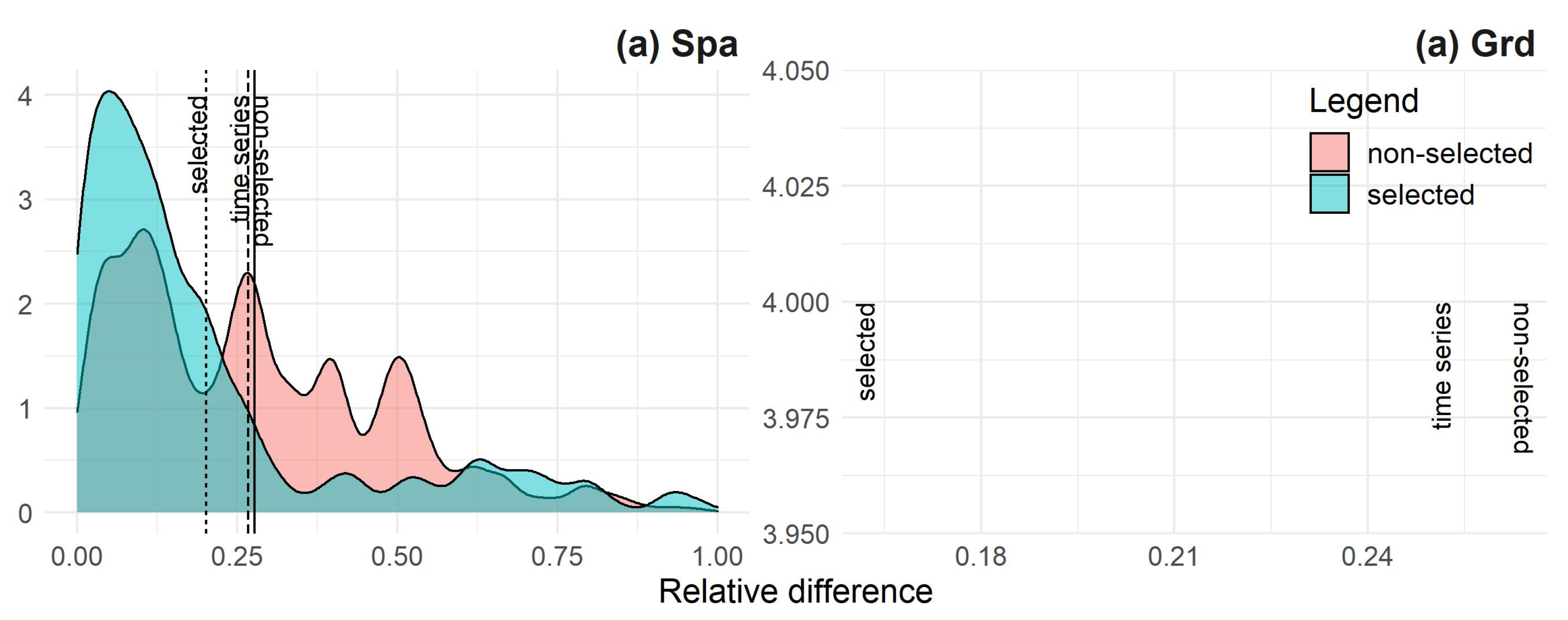
The relative error in fitted Spa and Grd parameters for groups of objective functions (OFs) with respect to expert calibration is given in

Table 3. Relative difference of Bilan model parameters Spa and Grd between expert calibration and other calibration strategies. Automatic, time series + signatures and signatures only mean calibration strategies which combinate runoff (R), soil moisture (SW) or runoff + soil moisture (R + SW).

BP	Automatic		Time Series + Signatures						Signatures Only
			R		SW		R + SW		R		SW		R + SW
	Mean	Median	Mean	Median	Mean	Median	Mean	Median	Mean	Median	Mean	Median	Mean	Median
Spa	0.202	0.121	0.204	0.122	0.282	0.285	0.275	0.267	0.243	0.163	0.297	0.269	0.305	0.272
Grd	0.163	0.158	0.164	0.161	0.388	0.363	0.233	0.169	0.232	0.148	0.391	0.358	0.252	0.164

. These two parameters are important for the characterization of hydrological balance of a catchment, representing the soil water retention (Spa parameter) and ground water response (Grd parameter).

For the Spa parameter, the best results are obtained with automatic standard calibration. Very similar results are achieved with group R2. The Spa parameter is clearly improved by runoff signatures as indicated in Table 3. Including soil moisture leads to worse results (see groups SW, SW2, RSW, RSW2). The Grd parameter describing the groundwater dynamics was reliably estimated in the R2, RSW, RSW2 and A groups. In this case, the soil moisture signatures have improved the Grd parameter but only in combination with runoff.

The density of relative errors in Bilan Spa a Grd parameters with respect to expert calibration for all calibration strategies is given in Figure 5. Again, the distribution of the errors for the selected (best-performing) objective functions (OFs) is much more consistent then for the rest of the OFs. Particularly for the Spa parameter, it is obvious that the selected OFs avoid the attraction to different parameter values which is evident for the rest of OFs (see red area on the left of Figure 5).

4.4. Runoff Signatures

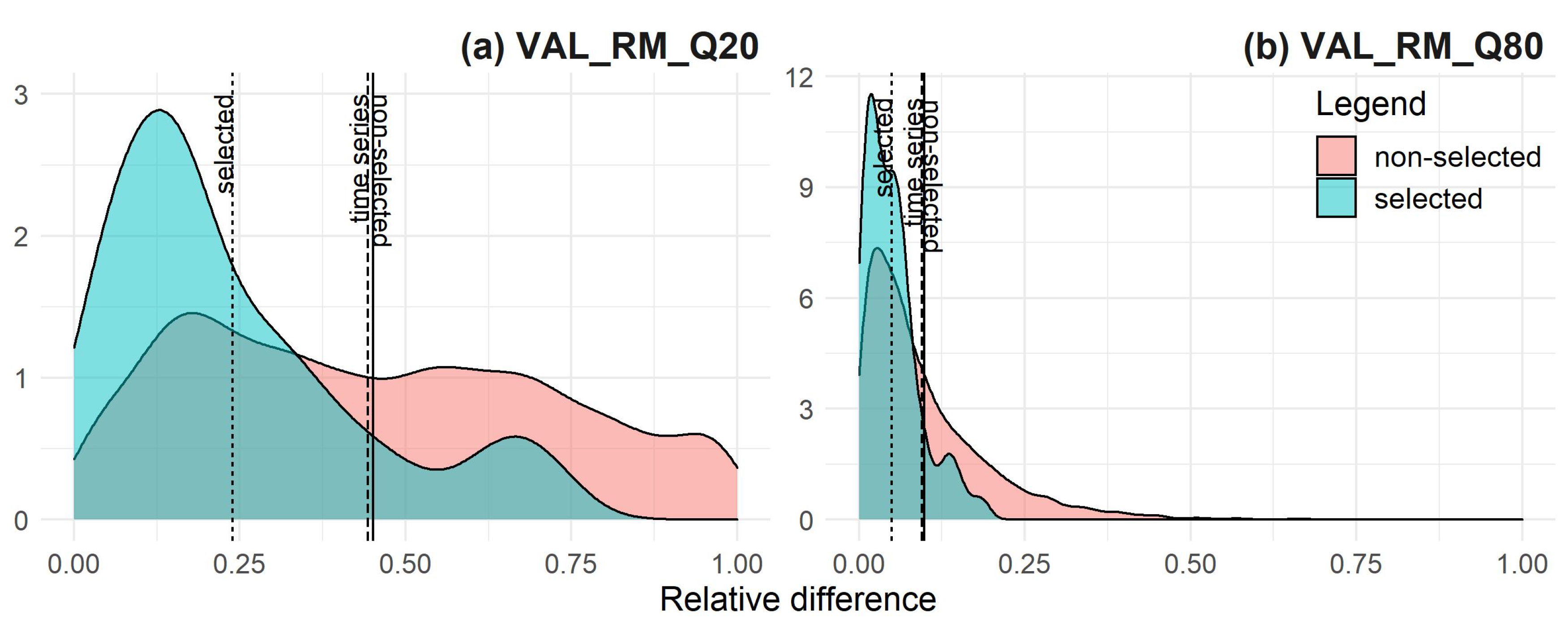
Lastly, we evaluated the performance of the calibration strategies with respect to low and high flows represented by the 20th (Q20) and 80th (Q80) percentile (

Table 4. Relative difference in Q20 and Q80 for runoff. Automatic, time series + signatures and signatures only mean calibration strategies which combinate runoff (R), soil moisture (SW) or runoff + soil moisture (R + SW).

RS	Automatic		Time Series + Signatures						Signatures Only
			R		SW		R + SW		R		SW		R + SW
	Mean	Median	Mean	Median	Mean	Median	Mean	Median	Mean	Median	Mean	Median	Mean	Median
Q20	0.224	0.172	0.225	0.181	0.568	0.570	0.391	0.323	0.354	0.299	0.545	0.565	0.482	0.439
Q80	0.075	0.056	0.073	0.057	0.182	0.159	0.114	0.087	0.141	0.106	0.221	0.173	0.155	0.127

). In the case of low flows, the performance of the model is clearly improved when runoff signatures are considered and even more so when this is done in combination with soil moisture signatures or time series. On the other hand, the standard automatic calibration ranked among the worst OFs. For the high flows in general, the differences is much less variable with automatic calibration being slightly better than the rest of the OFs.

The difference in the behavior between Q20 and Q80 is also obvious from the density presented in Figure 6 where the best performing OFs lead to a much narrower error distribution than the rest of the OFs for Q20, while the difference is very small in the case of Q80.

4.5. Summary of OFs’ Performance

The 52 OFs considered for calibration contain runoff (R, R2), soil moisture (SW, SW2), and both runoff and soil moisture (RSW, RSW2) as a time series or hydrological signatures. The OFs were assessed with respect to goodness-of-fit (GOF), uncertainty of Bilan model parameters (BP) and bias in runoff signatures (RS). To summarize the performance of different OFs, we ranked the OFs at each catchment according to GOF, BP and RS and checked which OFs appears most frequently. The set of those OFs is presented in

Table 5. The best OFs according to goodness-of-fit (GOF), parameters of the hydrological model (BP) and high and low flow indices (RS). Time series, R-signatures and SW-signatures mean characteristic which combined times series or signatures of runoff (R) and of soil moisture (SW), their statistic indicators are mean, interquartile range (IQR), sd and selected settings (*).

ID	Time Series		R-Signatures			SW-Signatures			Evaluation Metrics
	R	SW	mean	IQR	sd	mean	IQR	sd	GOF	BP	RS
automatic	*								*	*	*
R2-mean-sd			*		*					*
R2-mean-iqr			*	*						*	*
R2-mean-optim	*		*						*	*	*
R2-sd-iqr				*	*				*	*
R2-sd-optim	*				*				*	*
R2-iqr-optim	*			*					*	*	*
RSW-mean-mean			*			*			*	*
RSW-mean-iqr			*				*			*
RSW-sd-sd					*			*		*	*
RSW-optim-optim	*	*							*		*
RSW-optim-iqr	*			*					*		*
RSW-iqr-iqr				*			*				*
RSW2-sd-sd-optim		*			*			*		*
RSW2-optim-optim-sd	*	*						*	*		*
RSW2-optim-optim-mean	*	*				*			*		*
RSW2-optim-optim-iqr	*	*					*		*		*
RSW2-optim-mean-sd	*					*		*	*		*
RSW2-optim-iqr-sd	*						*	*	*		*
FDC-all	*								*	*	*
FDC-300-330-355-364	*								*	*	*

. There are only four OFs included in the best-performance set for all three criteria: the standard automatic calibration, R2-mean-optim and R2-iqr-optim. It is clear that time series information is crucial for hydrological simulation. However, the results also indicate that the OFs including hydrological signatures may rank among the best with respect to parameters of the hydrological model and low and high flow statistics. Our results suggest a relatively good agreement between modelled and observed runoff, however, when very low (Q80 and Q95) and very high quantiles for (Q20) are used for model diagnosis [4,25] it turns out that low flows (Q95–Q100) are significantly underestimated in most model settings.

This study was performed on 20 catchments, which means that the estimate of hydrological signatures may not be as robust as studies that include more catchments with diverse water regime allowing for better description of the behaviour of individual parameters, hydrological signatures, or selected variables [42]. Ref. [42] also mentiones, that the hydrological signatures are typically more influenced by climatic and topographic indices than by the land cover, soil properties, and geology. Although we did not consider other than hydroclimatic factors our study confirmed importance of the climatic factors especially those related to soil moisture influencing in particular low flows and groundwater-related parameter (Grd) of the Bilan model.

Similar to [17], we have shown that unconstrained calibrated model parameters are varying in wide range of implausible values and it is necessary to balance between automated model calibration with expert-knowledge and local system understanding strategy. In addition, the hydrological signatures, considerably narrow the range of parameter values and approach the expert-calibrated parameters well. Therefore they should be considered in the calibration and diagnostics of the model in particular when behavior of the extremes is of interest as was already suggested by [25].

5. Concluding Remarks

In the present paper, we assessed the performance of a conceptual runoff model (Bilan) calibrated using hydrological signatures based on long term runoff and soil moisture characteristics. The results of these strategies are compared to those of the standard automatic and expert calibration. The performance of tested combinations of runoff and soil moisture time series and signatures is evaluated with respect to goodness-of-fit (GOF) between simulated and observed runoff, uncertainty of the estimated Bilan model parameters (BP) and runoff signatures (RS) representing low and high flows.

The main findings can be summarized as follows:

• The standard automatic calibration performs best for most of the evaluation criteria, except for low flows;
• The objective functions (OFs) utilizing time series are always performing better than those based on signatures only;
• It is however clear that the good performance of automatically calibrated models can be counterbalanced by poor representation of hydrological processes, important hydrological signatures and overall increasing uncertainty of model parameters. Therefore, evaluation metrics accounting for biases in hydrological processes representation and objective functions combining the bias in runoff time series with that of other runoff characteristics should be considered;
• In the cases where the runoff time series are not available, it is possible to get sufficient fit even using signatures representing runoff mean and variability;
• The role of the runoff and soil moisture signatures is significant, in particular for low flows and parameters of the hydrological model.

The study was performed in specific conditions of the Czech Republic with a single hydrological model and further research is needed to confirm the findings also in different hydroclimatic and physical conditions and hydrological models.

References

- Madsen, H. Automatic calibration of a conceptual rainfall–runoff model using multiple objectives. J. Hydrol. 2000, 235, 276–288. [Google Scholar] [CrossRef]
- Merz, R.; Bloschl, G. Regionalisation of catchment model parameters. J. Hydrol. 2004, 287, 95–123. [Google Scholar] [CrossRef] [Green Version]
- Li, X.; Weller, D.E.; Jordan, T.E. Watershed model calibration using multi-objective optimization and multi-site averaging. J. Hydrol. 2010, 380, 277–288. [Google Scholar] [CrossRef]
- Pokhrel, P.; Yilmaz, K.K.; Gupta, H.V. Multiple-criteria calibration of a distributed watershed model using spatial regularization and response signatures. J. Hydrol. 2012, 418, 49–60. [Google Scholar] [CrossRef]
- Samuel, J.; Coulibaly, P.; Metcalfe, R.A. Estimation of continuous streamflow in Ontario ungauged basins: Comparison of regionalization methods. J. Hydrol. Eng. 2011, 16, 447–459. [Google Scholar] [CrossRef]
- Croke, B.F.W.; Merritt, W.S.; Jakeman, A.J. A dynamic model for predicting hydrologic response to land cover changes in gauged and ungauged catchments. J. Hydrol. 2004, 291, 115–131. [Google Scholar] [CrossRef]
- Oudin, L.; Andréassian, V.; Perrin, C.; Michel, C.; Le Moine, N. Spatial proximity, physical similarity, regression and ungaged catchments: A comparison of regionalization approaches based on 913 French catchments. Water Resour. Res. 2008, 44. [Google Scholar] [CrossRef]
- Masih, I.; Uhlenbrook, S.; Maskey, S.; Ahmad, M.D. Regionalization of a conceptual rainfall–runoff model based on similarity of the flow duration curve: A case study from the semi-arid Karkheh basin, Iran. J. Hydrol. 2010, 391, 188–201. [Google Scholar] [CrossRef]
- Zhang, Y.; Vaze, J.; Chiew, F.H.; Teng, J.; Li, M. Predicting hydrological signatures in ungauged catchments using spatial interpolation, index model, and rainfall–runoff modelling. J. Hydrol. 2014, 517, 936–948. [Google Scholar] [CrossRef]
- Biondi, D.; De Luca, D.L. Rainfall-runoff model parameter conditioning on regional hydrological signatures: Application to ungauged basins in southern Italy. Hydrol. Res. 2016, 48, 714–725. [Google Scholar] [CrossRef]
- Donnelly, C.; Andersson, J.C.; Arheimer, B. Using flow signatures and catchment similarities to evaluate the E-HYPE multi-basin model across Europe. Hydrol. Sci. J. 2016, 61, 255–273. [Google Scholar] [CrossRef]
- Qamar, M.U.; Azmat, M.; Cheema, M.J.M.; Shahid, M.A.; Khushnood, R.A.; Ahmad, S. Model swapping: A comparative performance signature for the prediction of flow duration curves in ungauged basins. J. Hydrol. 2016, 541, 1030–1041. [Google Scholar] [CrossRef]
- Visessri, S.; McIntyre, N. Regionalisation of hydrological responses under land-use change and variable data quality. Hydrol. Sci. J. 2016, 61, 302–320. [Google Scholar] [CrossRef] [Green Version]
- Havlíček, V.; Hanel, M.; Máca, P.; Kuráž, M.; Pech, P. Incorporating basic hydrological concepts into genetic programming for rainfall-runoff forecasting. Computing 2013, 95, 363–380. [Google Scholar] [CrossRef]
- Heřmanovský, M.; Havlíček, V.; Hanel, M.; Pech, P. Regionalization of runoff models derived by genetic programming. J. Hydrol. 2017, 547, 544–556. [Google Scholar] [CrossRef]
- Westerberg, I.K.; Wagener, T.; Coxon, G.; McMillan, H.K.; Castellarin, A.; Montanari, A.; Freer, J. Uncertainty in hydrological signatures for gauged and ungauged catchments. Water Resour. Res. 2016, 52, 1847–1865. [Google Scholar] [CrossRef] [Green Version]
- Hrachowitz, M.; Fovet, O.; Ruiz, L.; Euser, T.; Gharari, S.; Nijzink, R.; Freer, J.; Savenije, H.; Gascuel-Odoux, C. Process consistency in models: The importance of system signatures, expert knowledge, and process complexity. Water Resour. Res. 2014, 50, 7445–7469. [Google Scholar] [CrossRef] [Green Version]
- Pfannerstill, M.; Bieger, K.; Guse, B.; Bosch, D.; Fohrer, N.; Arnold, J. How to Constrain Multi-Objective Calibrations of the SWAT Model Using Water Balance Components. J. Am. Water Resour. Assoc. 2007, 53. [Google Scholar] [CrossRef]
- Tuo, Y.; Marcolini, G.; Disse, M.; Chiogna, G. A multi-objective approach to improve SWAT model calibration in alpine catchments. J. Hydrol. 2018, 599, 347–360. [Google Scholar] [CrossRef]
- McMillan, H.; Westerberg, I.; Branger, F. Five guidelines for selecting hydrological signatures. Hydrol. Process. 2017, 31, 4757–4761. [Google Scholar] [CrossRef] [Green Version]
- Farmer, D.; Sivapalan, M.; Jothityangkoon, C. Climate, soil, and vegetation controls upon the variability of water balance in temperate and semiarid landscapes: Downward approach to water balance analysis. Water Resour. Res. 2003, 39. [Google Scholar] [CrossRef]
- Yilmaz, K.; Gupta, H.V.; Wagener, T. A process-based diagnostic approach to model evaluation: Application to the NWS distributed hydrologic model. Water Resour. Res. 2008, 44. [Google Scholar] [CrossRef] [Green Version]
- Shafii, M.; Tolson, B. Optimizing hydrological consistency by incorporating hydrological signatures into model calibration objectives. Water Resour. Res. 2015, 51, 3796–3814. [Google Scholar] [CrossRef] [Green Version]
- Westerberg, I.; Guerrero, J.L.; Younger, P.; Beven, K.; Seibert, J.; Halldin, S.; Freer, J.; Xu, C. Calibration of hydrological models using flow-duration curves. Hydrol. Earth Syst. Sci. 2011, 15, 2205–2227. [Google Scholar] [CrossRef] [Green Version]
- Pfannerstill, M.; Guse, B.; Fohrer, N. Smart low flow signature metrics for an improved overall performance evaluation of hydrological models. J. Hydrol. 2014, 510, 447–458. [Google Scholar] [CrossRef]
- Tolasz, R. Atlas Podnebí Česka; ČHMÚ: Prague, Czech Republic, 2007; Volume 1. [Google Scholar]
- Hlavinka, P.; Trnka, M.; Balek, J.; Semerádová, D.; Hayes, M.; Svoboda, M.; Eitzinger, J.; Možný, M.; Fischer, M.; Hunt, E.; et al. Development and evaluation of the SoilClim model for water balance and soil climate estimates. Agric. Water Manag. 2011, 98, 1249–1261. [Google Scholar] [CrossRef]
- Mauricio Zambrano-Bigiarini. hydroGOF: Goodness-of-Fit Functions for Comparison of Simulated and Observed Hydrological Time Series, R Package Version 0.4-0. 2020.
- Tallaksen, L.M.; Van Lanen, H.A. Hydrological Drought: Processes and Estimation Methods for Streamflow and Groundwater; Elsevier: Amsterdam, The Netherlands, 2004; Volume 48. [Google Scholar]
- Vizina, A.; Horáček, S.; Hanel, M. Nové možnosti modelu Bilan. Vodohospodářské Technicko-Ekonomické Inf. 2015, 57, 7–10. [Google Scholar]
- Bárdossy, A. Calibration of hydrological model parameters for ungauged catchments. Hydrol. Earth Syst. Sci. Discuss. 2007, 11, 703–710. [Google Scholar] [CrossRef] [Green Version]
- Seibert, J. Estimation of parameter uncertainty in the HBV model: Paper presented at the Nordic Hydrological Conference (Akureyri, Iceland-August 1996). Hydrol. Res. 1997, 28, 247–262. [Google Scholar] [CrossRef]
- Jakubcová, M.; Máca, P.; Pech, P. Parameter estimation in rainfall-runoff modelling using distributed versions of particle swarm optimization algorithm. Math. Probl. Eng. 2015, 2015, 968067. [Google Scholar] [CrossRef] [Green Version]
- Vizina, A.; Hanel, M.; Novický, O.; Treml, P. Experience from Simulation of Climate Impacts on Water Regime in Monthly and Daily Time Step; TG Masaryk Water Research Institute: Prague, Czech Republic, 2010. [Google Scholar]
- Machlica, A.; Horvát, O.; Horáček, S.; Oosterwijk, J.; Van Loon, A.F.; Fendeková, M.; Van Lanen, H.A. Influence of model structure on base flow estimation using Bilan, frier and HBV-light models. J. Hydrol. Hydromechanics 2012, 60, 242–251. [Google Scholar] [CrossRef] [Green Version]
- Hanel, M.; Mrkvičková, M.; Máca, P.; Vizina, A.; Pech, P. Evaluation of simple statistical downscaling methods for monthly regional climate model simulations with respect to the estimated changes in runoff in the Czech Republic. Water Resour. Manag. 2013, 27, 5261–5279. [Google Scholar] [CrossRef]
- Vizina, A.; Hanel, M.; Trnka, M.; Daňhelka, J.; Gregorieová, I.; Pavlík, P.; Heřmanovský, M. HAMR: Online drought management system–operational management during a dry episode. Vodohospodářské Technicko-Ekonomické Inf. 2018, 60, 22–28. [Google Scholar]
- Duan, Q.; Sorooshian, S.; Gupta, V.K. Optimal use of the SCE-UA global optimization method for calibrating watershed models. J. Hydrol. 1994, 158, 265–284. [Google Scholar] [CrossRef]
- Storn, R.; Price, K. Differential evolution–a simple and efficient heuristic for global optimization over continuous spaces. J. Glob. Optim. 1997, 11, 341–359. [Google Scholar] [CrossRef]
- Chai, T.; Draxler, R.R. Root mean square error (RMSE) or mean absolute error (MAE)?—Arguments against avoiding RMSE in the literature. Geosci. Model Dev. 2014, 7, 1247–1250. [Google Scholar] [CrossRef] [Green Version]
- Gupta, H.V.; Kling, H.; Yilmaz, K.K.; Martinez, G.F. Decomposition of the mean squared error and NSE performance criteria: Implications for improving hydrological modelling. J. Hydrol. 2009, 377, 80–91. [Google Scholar] [CrossRef] [Green Version]
- Addor, N.; Nearing, G.; Prieto, C.; Newman, A.; Le Vine, N.; Clark, M.P. A ranking of hydrological signatures based on their predictability in space. Water Resour. Res. 2018, 54, 8792–8812. [Google Scholar] [CrossRef]
Figure 1.
Evaluated catchments.
Figure 2.
The Bilan hydrological model.
Figure 3.
Runoff ((a)-calibration, (b)-validation) relative difference probability curve (red line—manual calibration settings, green line—selected calibrations strategies, orange line—non-selected calibrations strategies).
Figure 4.
The density of differences in RMSE (a) and KGE (b) between expert calibration and the rest of the objective functions (OFs). The dotted line corresponds to mean of the selected best-performing OFs, the dashed line to the mean for the OFs, including time series, and the solid line to the mean of the OFs that were not selected.
Figure 5.
The density of relative errors in Spa (a) and Grd (b) based on selected best-performing OFs (green area) and the rest (red area). The dotted line correspond to the mean of the selected best-performing objective functions, the dashed line to the mean OFs, including time series, and the solid line to the mean of the OFs that were not selected.
Figure 6.
Density of error in runoff signatures in Q20 (a) and Q80 (b) based on selected best-performing OFs (green area) and the rest (red area). Dotted line correspond to mean of selected best-performing objective functions, dashed line to mean OFs including time series and the solid line the mean of the OFs that were not selected.