A New Runoff Routing Scheme for Xin’anjiang Model and Its Routing Parameters Estimation Based on Geographical Information


1
College of Hydrology and Water Resources, Hohai University, Nanjing 210098, China
2
State Key Laboratory of Hydrology-Water Resources and Hydraulic Engineering and CMA-HHU Joint Laboratory for HydroMeteorological Studies, Hohai University, Nanjing 210098, China
*
Authors to whom correspondence should be addressed.
Water 2020, 12(12), 3429; https://doi.org/10.3390/w12123429
Submission received: 3 November 2020
/
Revised: 3 December 2020
/
Accepted: 4 December 2020
/
Published: 6 December 2020
(This article belongs to the Special Issue Advanced Hydrologic Modeling in Watershed-Scale)
Abstract
:The Xin’anjiang model is a conceptual hydrological model, which has an essential application in humid and semi-humid regions. In the model, the parameters estimation of runoff routing has always been a significant problem in hydrology. The quantitative relationship between parameters of the lag-and-route method and catchment characteristics has not been well studied. In addition, channels in Muskingum method of the Xin’anjiang model are assumed to be virtual channels. Therefore, its parameters need to be estimated by observed flow data. In this paper, a new routing scheme for the Xin’anjiang model is proposed, adopting isochrones method for overland flow and the grid-to-grid Muskingum–Cunge–Todini (MCT) method for channel routing, so that the routing parameters can be estimated according to the geographic information. For the new routing scheme the average overland flow velocity can be determined through the land cover and overland slope, and the channel routing parameters can be determined through channel geometric characteristic, stream order and channel gradient. The improved model was applied at a 90 m grid scale to a nested watershed located in Anhui province, China. The parent Tunxi watershed, with a drainage area of 2692 km2, contains four internal points with available observed streamflow data, allowing us to evaluate the model’s ability to simulate the hydrologic processes within the watershed. Calibration and verification of the improved model were carried out for hourly time scales using hourly streamflow data from 1982 to 2005. Model performance was assessed by comparing simulated and observed flows at the watershed outlet and interior gauging stations. The performance of both original and new runoff routing schemes were tested and compared at hourly scale. Similar and satisfactory performances were achieved at the outlet both in the new runoff routing scheme using the estimated routing parameters and in the original runoff routing scheme using the calibrated routing parameters, with averaged Nash-Sutcliffe efficiency (NSE) of 0.92 and 0.93, respectively. Moreover, the new runoff routing scheme is also able to reproduce promising hydrographs at internal gauges in study catchment with the mean NSE ranging from 0.84 to 0.88. These results indicate that the parameter estimation approach is efficient and the developed model can satisfactorily simulate not only the streamflow at the parent watershed outlet, but also the flood hydrograph at the interior gauging points without model recalibration. This study can provide some guidance for the application of the Xin’anjiang model in ungauged areas.
1. Introduction
The watershed hydrological model is a significant tool for hydrological simulation. At present, hydrological models are mainly divided into conceptual models and physically based distributed models. Conceptual hydrological models generalize runoff generation and runoff routing processes based on the mass conservation and experimental simulation or empirical function relationship. The conceptual model is simple and easy to be established, but the parameters are difficult to be determined by the theoretical formula. Generally, it needs to be calibrated according to the observed flow [1,2], which limits the application of the conceptual model in ungauged areas. For the physically-based distributed hydrological models, their parameters can be estimated by catchment characteristics and meteorological conditions, which is able to fully consider the influence of soil, land use types and terrain characteristics, and better describe the spatial variability of watershed. However, due to the problems of over parameterization and scale, the use of complex models does not necessarily lead to better hydrological simulation results at watershed outlet [3,4,5,6,7]. In view of the advantages and disadvantages of conceptual hydrological models and physically based distributed hydrological models, Robinson et al. [8] suggested reconsidering the use of simpler approaches and found connections between physically based and conceptual models. Later on, Koren et al. [4] investigated an approach that combined the features of a widely used the conceptual SAC–SMA model and physically based kinematic routing model in the development and parameterization of a modeling system referred to as HL-RMS. A modeling framework in which lumped, semi-distributed and fully distributed approaches could be constructed and tested was provided in their study. The procedures for deriving a priori parameters as well as the computational efficiency of the HL-RMS have been supported by the Distributed Model Intercomparison Project (DMIP) [9,10]. Moore et al. (2006) [11] developed a conceptual-physical area-wide model (e.g., the G2G model) supported by terrain and soil property data, and demonstrated the potential value of distributed conceptual-physical models for flood warning and for identifying flood prone locations.
The Xin’anjiang model is a popular conceptual hydrological model in China. Since it was first developed in the 1970s, it has been widely used in humid and semi-humid areas, and has been employed into China’s national flood forecasting system [12,13]. However, the determination of sensitive parameters is a significant problem for the model. Generally, it is difficult to estimate these parameters by geographical information so that these parameters have to be calibrated through historical observation especially runoff routing parameters. For instance, the river network recession constant Cs [14] of the lag-and-route method represents the retention and storage capacity of river network and quantifies the flood peak attenuation. It has been widely recognized that the simulated flood events by the Xin’anjiang model are extremely sensitive to this parameter. Generally, the value of Cs related to catchment drainage area, river network topology, overland slope and flow velocity, etc. Although many studies have applied to the estimation this parameter values, they have some limitations. For example, Zhao [15] deduced the equation of Cs with the change of the reference river length and flow velocity from the analysis of physical mechanism, but the method still needs to rely on the observed hydrological data. Later, some scholars utilized a statistical method to study the relationship between Cs and geomorphic characteristics. For example, Xu et al. [16] calibrated the parameters of 13 watersheds by observed data in Huangshan area, China, and obtained the empirical relationship between Cs and drainage area. Hu et al. [17] extracted 10 underlying surface factors of 29 watersheds in Southern Anhui province, China, and then established the regression relationship between Cs and the underlying surface characteristics. However, these methods can only achieve good simulation results for catchments with similar hydrological properties as studied catchments. Therefore, it is difficult to apply these methods to other catchments. Besides, the parameter Lag, another important parameter controlling the river network routing in the Xin’anjiang model and influencing flood propagation and peak time, is also not easy to estimate due to lack of clear physical meaning. What is more, the Muskingum method [18] employed by the Xin’anjiang assumes that the channel is a virtual channel so that its parameters cannot be estimated by channel characteristics and hydraulic properties. Specifically, it is generally known that the time constant Ke of Muskingum method is identical to concentration time interval of the sub catchment, and another parameter x still needs to be calibrated by observation. Overall, it is challenging to apply the Xin’anjiang model in ungauged area.
With the development of Digital Elevation Model (DEM) technology, more geographic data (river channel topology, slope and underlying surface characteristics) can be obtained. Some runoff routing schemes with physical basis of routing methods have been developed based on DEM for the Xin’anjiang model over the years. For example, Yao [19] proposed the distributed Grid-Xinanjiang model, a distributed conceptual-physical model. It successfully applied the grid-based model to two Chinese catchments for the simulation of hydrologic processes and demonstrated that the model has the capability of providing valuable spatial distributions of hydrologic variables. A physically based approach using geographically based information for a priori parameter estimates was presented as well, and it was proved that the proposed method is effective [20]. However, the parameters in the model are more complex and the scale of model parameters needs further study. In addition, to improve the flood prediction capability of the Xinanjiang model in ungauged nested catchments, Yao [21] used the concept of geomorphic unit hydrograph (GIUH) with physical basis to improve the Xin’anjiang model, and established the Xin’anjiang (XAJ)-GIUH model. However, it still uses the Muskingum method for channel routing, so its parameter must be calibrated in ungauged area.
The purpose of this paper is to determine a simple, efficient and reasonable routing approach by combining the conceptual and distributed model feature so that the model parameters can be estimated by geographical information. The isochrone method [22,23,24] was chosen in this paper to replace the lag-and-route component of the Xinanjiang model. It has the advantage of requiring a limited number of parameters whereas the necessary geomorphologic data can be obtained from DEM. Furthermore, we used the grid-to-grid Muskingum–Cunge–Todini (MCT) method [25,26] for channel routing. The MCT method was selected to improve the channel routing module of the Xin’anjiang model for the following reasons: First, it can guarantee the mass conservation in the calculation process. Second, its parameters can be determined according to the river channel geometric characteristics and hydraulic properties. Third, MCT method can be easily programmed and have high computation efficiency.
This paper is organized as follows: the methodology of the new catchment scheme is proposed in the Section 2; a concise description of the research catchment is given, and data sources and model comparison methods are proposed in Section 3; In Section 4, the improved model and Xin’anjiang model are applied to the study catchment, and the simulation results of the two models are compared and discussed; additionally, the model’s ability to predict hydrologic processes at interior points without model recalibration is evaluated. The last section gives a summary and more discussions on the limitations and future directions for improvements.
2. Methodology
2.1. Xin’anjiang Model
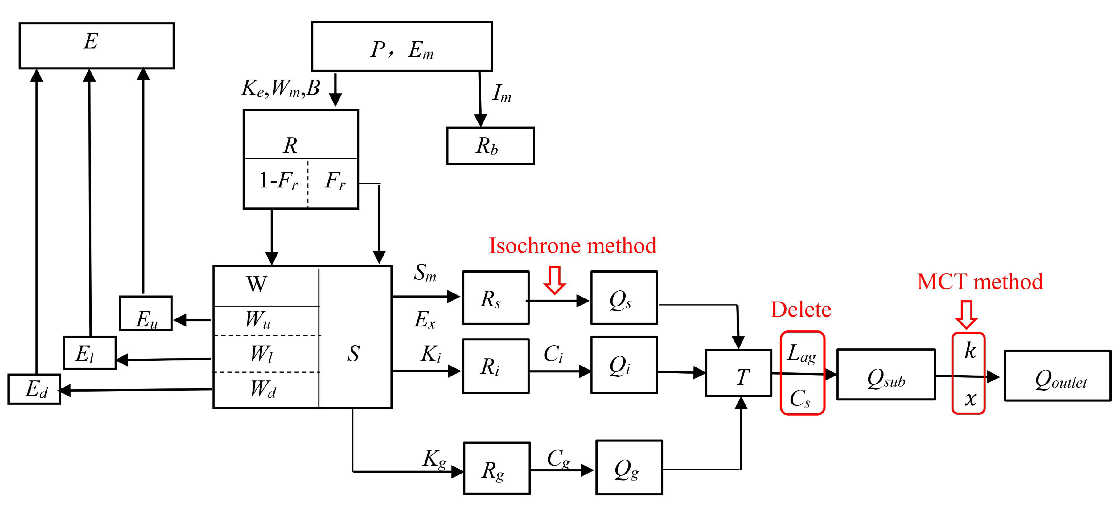
The Xin’anjiang model, developed in the 1970s, is a semi-distributed conceptual rainfall-runoff model. The catchment is divided into a set of sub-catchment, allowing the spatial patterns of inputs to be taken into account at the sub-catchment level. The main feature of the Xin’anjiang model is the concept that the aeration zone reaching its field capacity causes infiltration excess runoff without further loss. For each sub-catchment, the sub-catchment runoff is calculated using four major modules: evapotranspiration module, runoff generation module, runoff separation module and runoff routing module (Figure 1). In the runoff routing module, the overland flow directly flows into the river network of each sub catchment due to quick surface flow, while the interflow and the underground flow are slow, they first pass through the regulation and storage of linear reservoir and then converge into the river network. The total runoff into river network (including surface flow, interflow and groundflow) is routed to the outlet of each sub catchment by means of the lag-and-route method. Sub-catchment runoff routing for producing the catchment runoff is described by the Muskingum successive-reaches model. The river reach is normally sub-divided into sub-reaches in this successive routing scheme. More details about the Xinanjiang model can be found in Zhao (1992) [14].
2.2. The New Runoff Routing Scheme
A new runoff routing scheme is developed based on the original Xin’anjiang model. As shown in Figure 1, the parts marked in red represent where the model was modified. In the new runoff routing scheme, the isochrone method is utilized for calculating the amount of overland runoff flowing into the main river channel in each sub catchment during each interval. The interflow and groundwater runoff are routed to the main channel through linear reservoirs at every period. The grid-to-grid MCT method, instead of the original Muskingum method, is employed to channel routing. Comparing the lag-and-route method and Muskingum method of the original runoff routing module, the isochrone method can be easily derived from the routing paths, overland roughness and slope in terms of the DEM and land cover analysis; parameters of MCT can be easily determined by the channel geometric characteristic, channel roughness and channel gradient according to DEM and stream order. The following is a brief description of the new runoff routing scheme.
2.2.1. Overland Routing
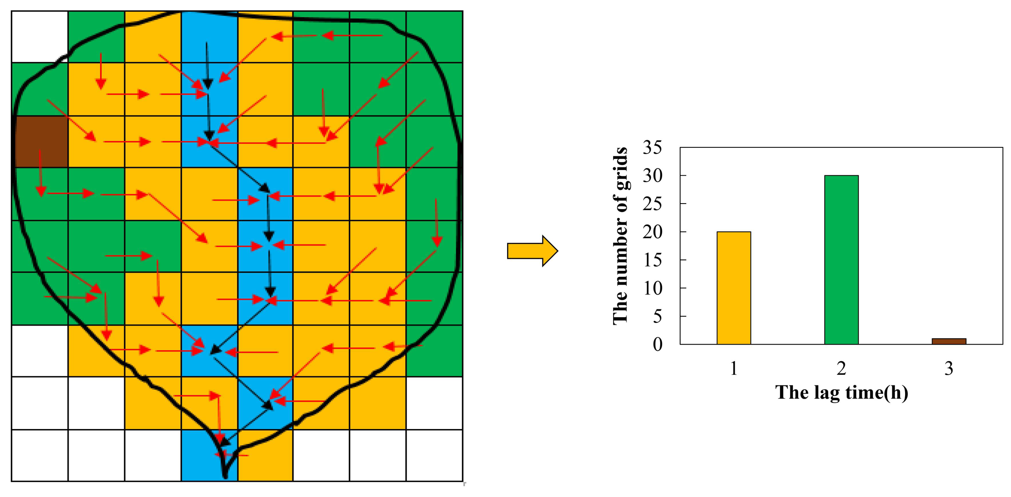
A rainfall can be regarded as a lot of water droplets, and it falls all over the catchment randomly. After deducting the loss, the water drops fallen into the catchment will choose a flow path and take some time to arrive at the outlet of the catchment [27,28,29,30]. This travel time is the lag time of the droplet. In this paper, the runoff generated by a rainfall in a grid are assumed to be a water droplet. The size of the water droplet can be set by adjusting the size of the grid cell. In the catchment runoff routing process, the overland runoff is assumed to be equal in every grid droplet, and the flow process from all grid droplet to main channel at each sub catchment can be calculated by isochrone method. A rainfall was supposed to be composed of water droplets. For any water droplet , if the length of the flow path from water droplet to the channel grid cell is , and the flow velocity is recorded as , then the lag time of the droplet in the catchment is
where, is the travel time of the droplet ; is the routing path.
If the rainfall falls on the catchment at Time , only those water droplets whose concentration time is exactly equal to can reach the outlet section of the drainage catchment at Time , and constitute the discharge of the drainage catchment outlet at Time . If it is assumed that the spatial distribution of rainfall over each sub catchment is uniform, the net precipitation is , so
where, is the discharge of Time at the outlet of the drainage catchment formed by precipitation at Time 0; is the indicator function. When , its value is 1, indicating that the water droplets whose concentration time belong to Time are the contributors to the outlet flow at Time ; otherwise, the value is 0, indicating that the water droplets whose concentration time do not belong to Time cannot be the contributor to the outlet flow at Time ; is the area occupied by the water droplet .
For a rainfall process, Formula (2) can be repeatedly used at different rainfall periods, and then the discharge hydrograph of the outlet can be obtained by superposition principle. The key to this method is to determine the flow path and velocity. The flow path of each water droplet can be determined by the flow direction analysis. The eight directions (D8) method [31], in which the flow direction is determined by one of the eight neighbors according to the steepest downward slope, is widely used to construct flow network because of its simplicity. For example, the flow path networks used in the River Transport Model (RTM) [32], the Total Runoff Integrating Pathways (TRIP) model [33], the overland flow routing module in the Hydrology Laboratory Research Modeling System (HL-RMS) of the US national weather service [4,34], and the routing module in the Three-layer Variable Infiltration Capacity (VIC-3L) model [35] are all generated based on the D8 method. These examples suggest that the D8 method is sufficient for flow direction analysis to achieve satisfactory accuracy. The specific steps of overland routing are as follows.
In the first step, the river channel of catchment and flow direction were extracted based on a high-resolution DEM (90 m × 90 m) by ArcGIS software.
In the second step, the natural sub catchments division method was used to divide the units and ensured that each sub catchment contains a rainfall station. The channels from the outlet of each sub catchment to the outlet of the whole catchment were reserved, and other river channels were deleted, in which the reserved river channels were used for channel routing calculation.
In the third step, as shown in Figure 2, according to D8 method, the lengths of routing path from each overland cell grid to river reach were obtained, so the lag time histogram of each sub catchment was obtained. Shapes of the histograms for each sub catchment are generally different from each other, indicating relatively different physical information associated with landscape topology. For example, a larger number of the grid cells are associated with long lag time, which indicates that a large number of grid cells within this sub catchment are far away from the channel and thus, their flow lengths are relatively large. In contrast, if many of the overland grid droplet are associated with relatively short lag time, indicating that a large number of overland grid cells are close to the channel.
Information of the lag time histograms for each sub catchment were employed to determine what percentage of the overland flow would be arrived at the river channel at each time step based on the corresponding calculated overland flow velocity. Therefore, the determination of flow velocity is crucial in overland routing. The overland flow is neither dominated by the internal interaction of the flow as that of the channel flow, nor is it mainly affected by the surrounding solid boundary like the soil pore flow, but is a flow dominated by the internal interaction of the flow and affected by the surrounding solid boundary. Hence a form between the Manning formula and Darcy formula can be considered in the form of overland velocity formula. A simplification of the Manning formula was employed to estimate the overland velocity:
where is overland flow velocity; is the multiplier on overland Manning’s roughness; is overland Manning’s roughness coefficient; is the average overland slopes.
2.2.2. Interflow and Groundwater Routing
The linear reservoir method in the Xin’anjiang model was still employed for interflow and groundwater routing, and the formulas are shown in (3) and (4):
where, and are interflow and groundwater runoff at time , respectively; is recession constant of lower interflow storage; is recession constant of groundwater storage; and ; is subwatershed area (km2); is the time interval of sub catchment concentration, which is usually set as 1h in Xin’anjiang model.
The total amount of runoff (including surface flow, interflow and groundflow) that reached the main river channel in each interval was distributed equally to each river channel reach, which was used as the lateral inflow to participate in the channel routing.
2.2.3. Channel Routing
Channels were regarded to be rectangular. Assuming the channel grid cell size was (m), the routing distance between the adjacent upstream and downstream grid cells is defined as the distance between the center points of the river channel grid cells, which is equal to (orthogonal flow direction) or 2 (diagonal flow direction). We assigned an ID to each river reach and the ‘1′ to the outlet of the whole catchment. According to the flow direction file, the inflow grids were searched from the downstream to the upstream according to the D8 principle. These grids were numbered ‘2′, ‘3′, ‘4′…, respectively until the source of each river branch was found. If two inflow cell grids were found in the search, the two inflow cell grids would have the same code.
According to the numbering sequence, the MCT method was used to calculate the flow from the river channel to the outlet of the catchment. At the junction, the discharge routed from upstream tributaries was added together, then the added discharge was routed to next downstream junction. For the MCT method, correction factors , corrected Courant number and Reynolds number were introduced to ensure mass conservation [25,36]. Flow in each channel grid cell is modeled as
where is wave celerity (m/s); is channel flow cross-sectional area (m2); B is channel width (m); is wetted perimeter (m); is the reference discharge (m3/s); is the distance between two adjacent upstream and downstream grid cells (m); is the time interval of channel routing (s); is channel bed slope (dimensionless).
The reference water level and wave velocity were obtained by a Newton–Raphson method with the following implicit equations:
where is the reference discharge (m3/s); is channel Manning’s roughness coefficient; is the channel slopes were to take the average slopes of longest flow path traced from DEM at different locations over the sub catchment.
where and are the inflow at the start and the end time (m3/s); and are the outlet flow at the start and the end time (m3/s); is lateral inflow (including surface, interflow and groundwater flow) per unit length of channel (m2/s); is the distance between two adjacent upstream and downstream grid cells (m).
2.2.4. Routing Parameters Estimation for New Routing Scheme
The estimation of model parameters is very critical for the application of the model in ungauged area. According to Figure 1, the routing parameters in Xin’anjiang model include , , , Lag, and , which must be calibrated by observed flow. The routing parameters in the new runoff routing module include , , , , , , and B, in which, the values of , and , are set according to valuable operational experience with the Xinanjiang model; parameters , , , and B can be estimated according to DEM, land cover classification and river stream order. However, there is large uncertainty associated with the Manning’s roughness coefficient. Therefore, the multiplier on Manning’s roughness needs to be calibrated by observed discharge of outlet. The specific calculation equations of , , , and B are as follows.
Overland slope:
where is the number of the overland grid over the sub catchment. is the elevation difference between the grid cell and corresponding channel grid cell, is the length of the routing path of grid cell .
For the initial values of overland roughness and channel roughness , These two parameter ranges mainly refer to the parameter value determination given in the Weather Research and Forecast (WRF)-Hydro model [37]. Overland Manning’s roughness coefficients were estimated by cover land characteristics for overland flow, while for channel routing coefficients were initialized for the stream order.
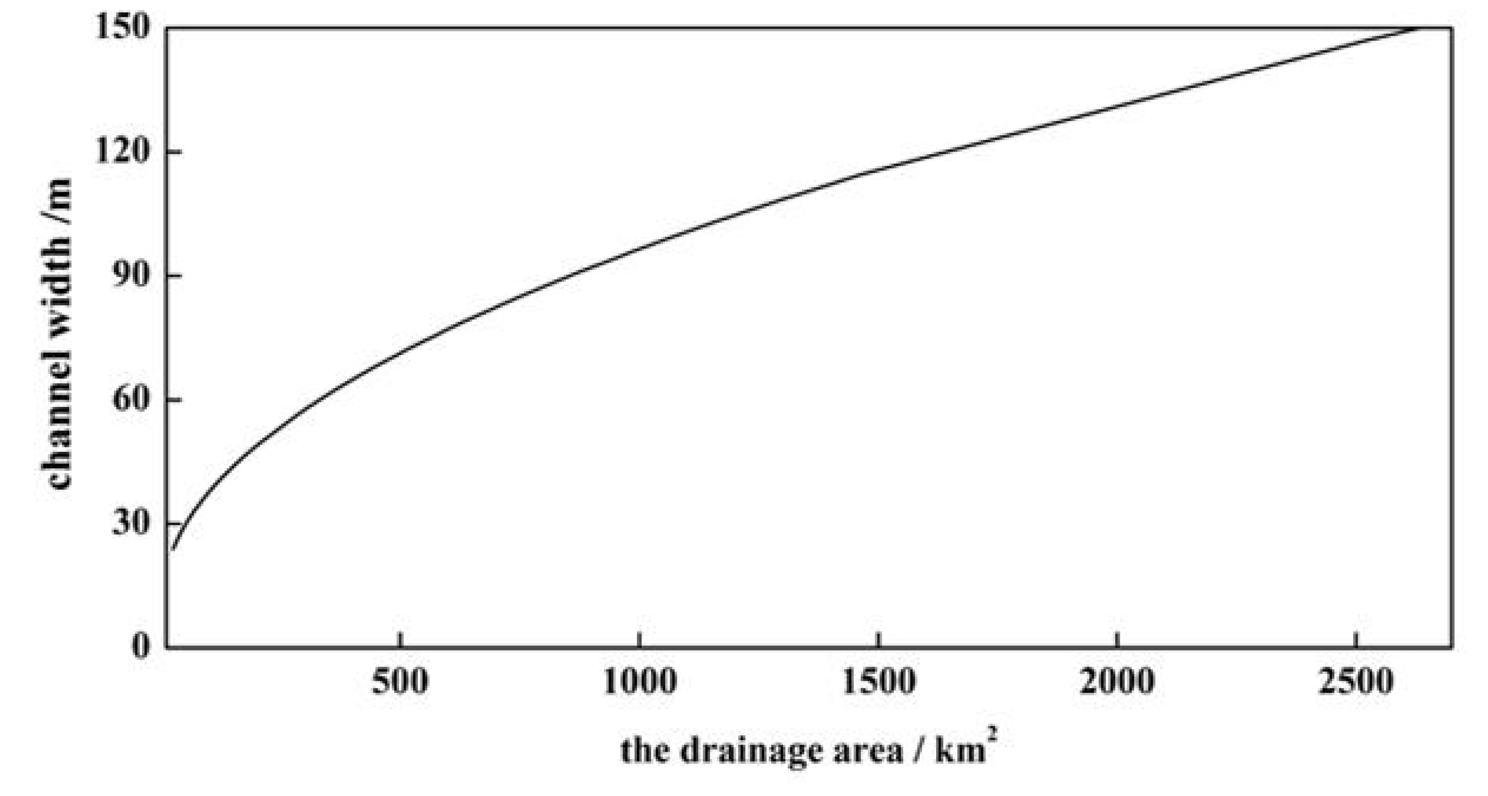
The channel width formula of the TOPKAPI model was used to calculate the width of river grid because only drainage area involved in the formula, which can be easily obtained from DEM [26]. The channel width (, in m) at channel grid cell is taken to increase as a function of the area drained by grid cell on the basis of geomorphological considerations:
where, and are the maximum and minimum width of cross sections in all of sub-reaches, respectively (m); is the minimum drainage area forming the river (km2); is the total drainage area of a catchment (km2); and is the drainage area of grid cell (km2).
The channel bed slope and channel friction slope at grid were approximated by forward difference at the front grid :
where, is the bottom slope; is the bottom elevation of the river (m); is the distance between the center of cell and j (m).
3. Case Studies
3.1. Studies Area
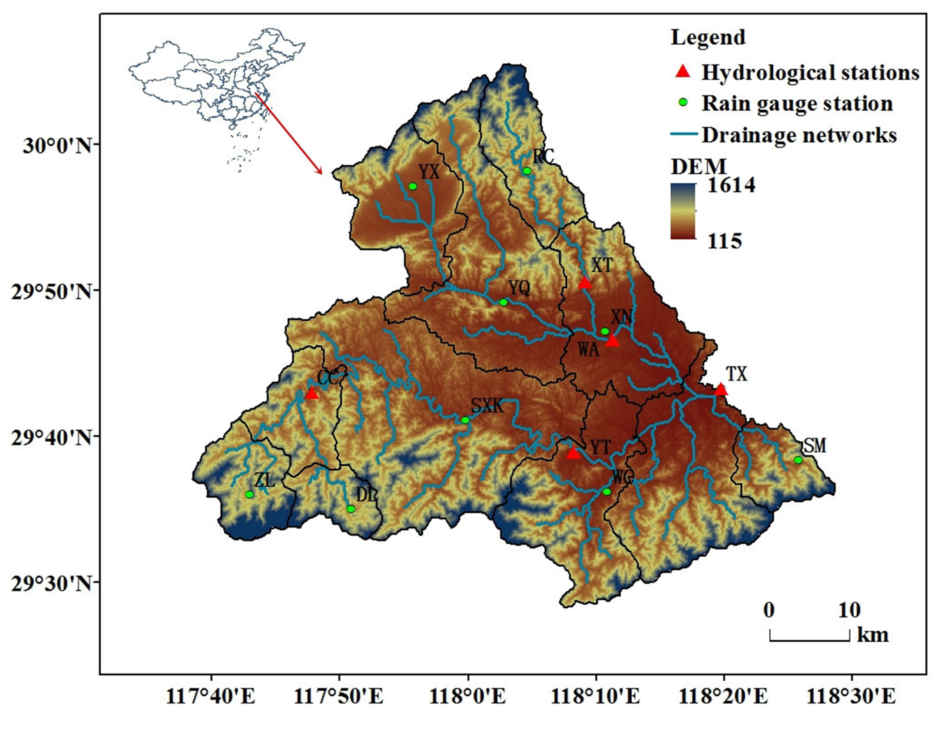
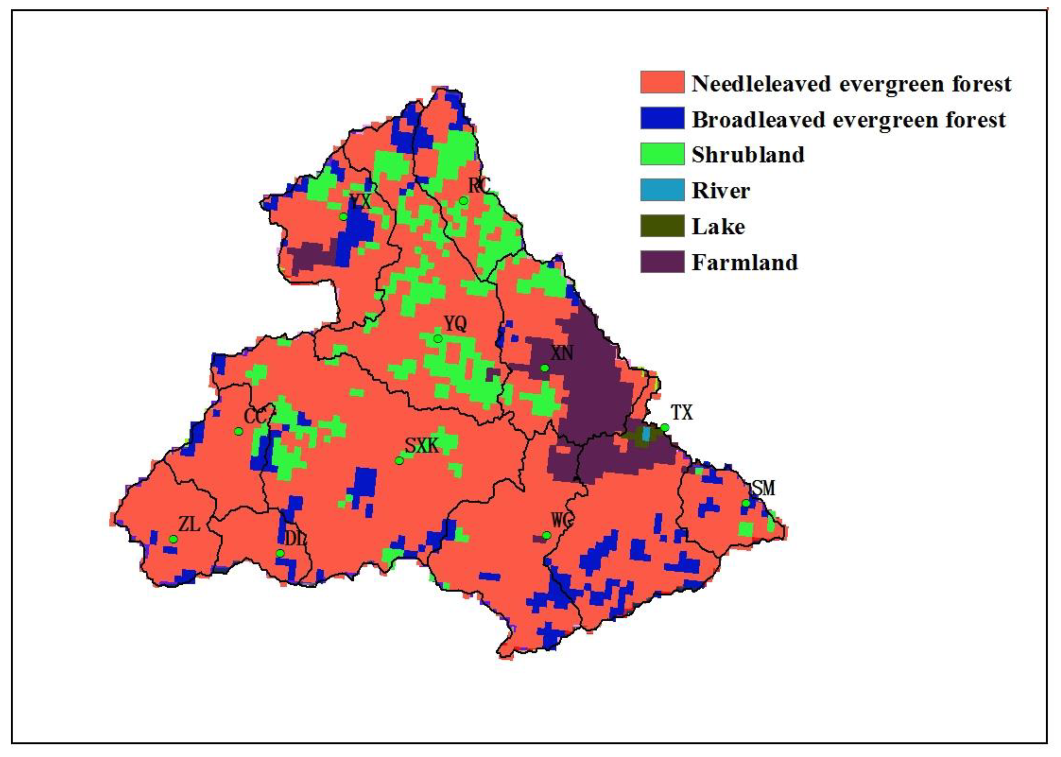
The Tunxi catchment, a typical wet area, located in the southern mountainous region of Huangshan City, Anhui Province, China, was selected as the study area. The terrain is high in the south and low in the north with elevation in the range of 115 to 1614 m. Its 2692 km2 drainage area has a monsoon dominant climate with more than 60% of annual rainfall during the flood season (May to August). The long-term annual average rainfall from 1982 to 2005 is 1600 mm yr−1. River discharge varies seasonally and inter-annually. Floods in the Tunxi catchment have the characteristics of high peak flow and short duration. Apart from the hydrological station at the outlet of the Tunxi (TX) catchment, there are four interior hydrological stations called Chengcun (CC), Yuetan (YT), Xinting (XT) and Wanan (WA), nine rain gauge stations including Wucheng (WC), Shimen (SM), Zuolong (ZL), Dalian (DL), Shangxikou (SXK), Rucun (RC), Yixian (YX), Yanqian (YQ) and Xiuning (XN) (Figure 3). The period of flood events and number of selected flood events were listed in Table 1. Digital elevation map (DEM) data with a 90 m × 90 m resolution are provided by Geospatial Data Cloud site, Computer Network Information Center, Chinese Academy of Sciences (http://www.gscloud.cn/). In terms of The Land Cover Map for China in the Year 2000 (http://www.gvm.jrc.it/glc2000), vegetation types of the catchment were classified into Needleleaved evergreen forest, Broadleaved evergreen forest, Shrubland, River, Lake and Farmland (Figure 4).
3.2. Model Evaluation and Comparison
To assess the new runoff routing schemes and understand its behavior, it is valuable to compare it with the original runoff routing scheme of the Xin’anjiang model. The performance of both the original and new runoff routing schemes were tested and compared at hourly scale in the Tunxi catchment with four interior hydrological stations. 32 floods from 1981 to 2005 were selected for simulation calculation. The first 19 floods were used for calibration and the remaining 13 floods for verification in Xin’anjiang model. Since this paper only studies the influence of different routing scheme on the simulations, all parameters of the improved model were the same as those of Xin’anjiang model except the routing parameters , , , , and B. Estimation methods in Section 2.2.4 were utilized to estimate these routing parameters. There were four internal locations (Yuetan, Wanan, Chengcun and Xinting) in the Tunxi catchment that were modeled as ‘‘ungauged’’ but had measured streamflow data to use for testing the improved model’s abilities to blindly simulate rainfall-runoff responses at the “ungauged’’ points. It should be noted that the observed streamflow data at the interior points were not used for the calibration and validation process. We chose 33, 22, 25 and 27 flood events in Yuetan, Wanan, Chengcun and Xinting which were used for verification respectively.
In accordance with the accuracy standard established by Ministry of Water Resources of the People’s Republic of China (MWR) [38], four metrics were chosen as evaluation criteria including relative runoff volume error (RRE, %), relative peak discharge error (RPE, %), peak time error (PTE, h) and Nash–Sutcliffe efficiency (NSE) [39]. The simulation qualified relative to total runoff volume, peak discharge, peak time and NSE if the absolute value of RRE was less than 20%, if the absolute value of RPE was less than 20%, if the difference in peak time was within the routing period or 3 h, respectively, and if the NSE was greater than 0.7.
where is the observed runoff volume; is the simulated runoff volume; is the observed peak discharge; is the simulated peak discharge; is the observed time of flood peak; is the simulated time of flood peak; is the observed discharge for each time step t; is the simulated or predicted value at time ; is the observed mean within the time period of analysis; and is the total number of values.
4. Results and Discussion
4.1. Parameter Calibration and Estimation
The Xinanjiang model involves a total of 17 parameters, which are listed in Table 2. The improved model shares 13 of the 17 Xinanjiang model parameters. The CS and Lag of the lag-and-route method and and of the Muskingum method in the original Xinanjiang model are not needed in the improved model. Instead, parameters , , , , and B are introduced in the improved model. The overland roughness and channel roughness were estimated according to the WRF-hydro download repository. For example, the values of for the six land cover types of the Tunxi catchment were 0.2 (Needleleaved evergreen forest), 0.2 (Broadleaved evergreen Forest), 0.055 (Shrubland), 0.055 (Grassland), 0.025 (Urban and Built-Up Land) and 0.005 (Water Bodies). The overland roughness of each sub catchment was obtained according to the area weight of each land cover type. The channel roughness was determined according to the stream order. The average overland slope of longest flow path traced from the DEM at different locations over each sub catchment was regarded as the average overland slope. Manning’s roughness coefficient values and overland slopes of Tunxi sub catchments were listed in Table 3. The value of the multiplier on overland Manning’s roughness was calibrated to be 0.51 by observed flow. Google Earth was employed to measure the minimum river width and the maximum river width of Tunxi catchment, which are 20 m and 150 m respectively, so that the river width of each channel grid was obtained according to Formula (17). The relationship between river width and upstream drainage area in Tunxi catchment is shown in Figure 5.
4.2. The Performance of the New Routing Scheme at the Outlet
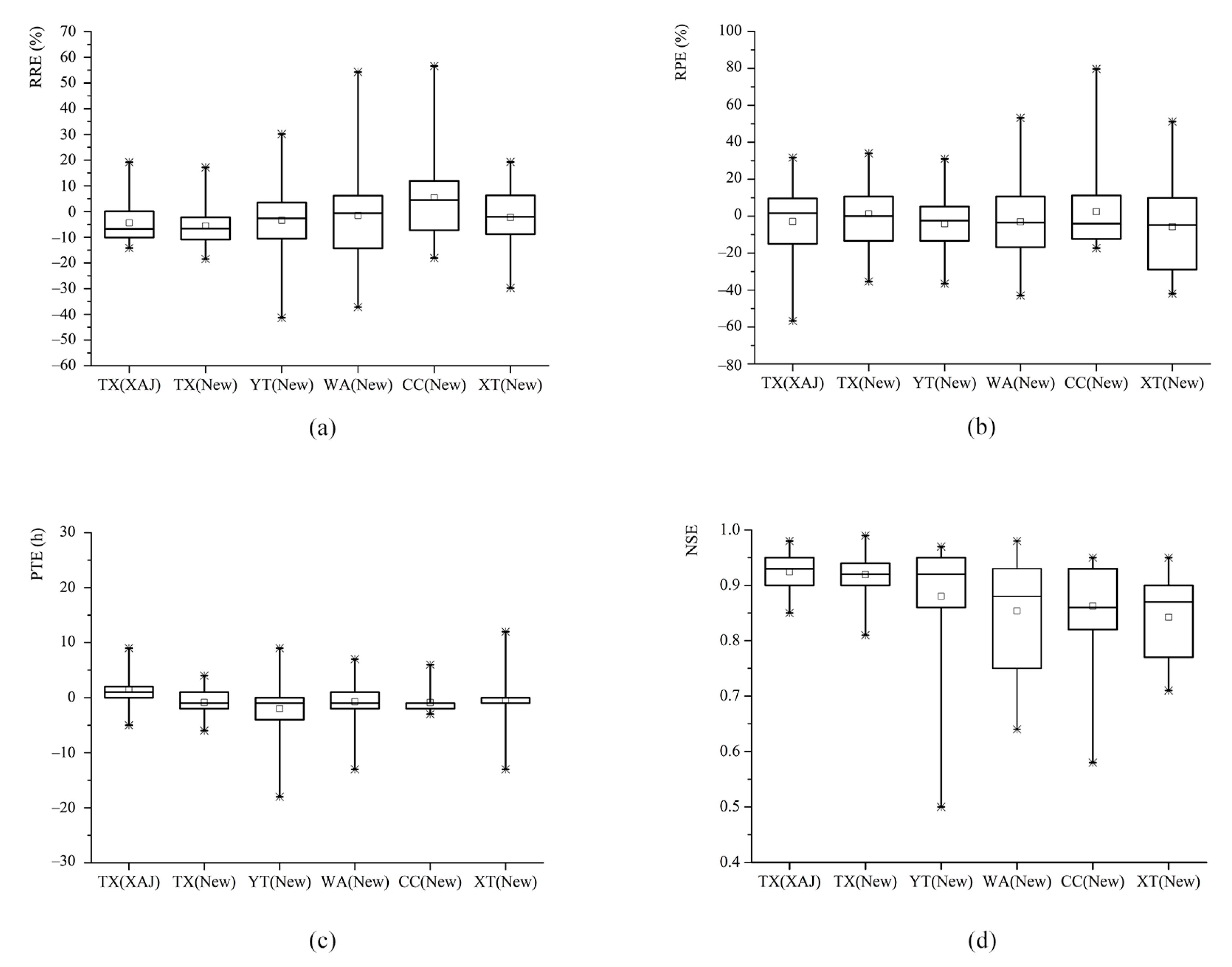
Figure 4 shows the distributions of RRE, RPE PTE and NSE statistics for all flood event simulations (both calibration and validation periods) by using the Xin’anjiang model and improved model. The top and bottom lines of these box plots represent the maximum and minimum values, respectively, while the top, middle, and bottom of the box represent the 75th percentile, 50th and 25th percentile, respectively. We evaluated the performance of the improved model by comparing the simulation results using both the Xin’anjiang model and improved model. For the outlet TX, the RRE values of the simulations by the Xin’anjiang model generally ranged between −15% and 20%, while these values of the simulations by the improved model mainly varied between −18% and 17% (Figure 6a); RPE values for the simulations by the Xin’anjiang model fell between −60% and 27% with a mean value of −2.83%, while RPE values for the simulations by the improved model fell between −36% and 34% with a mean value of 1.22% (Figure 6b); PTE values of simulations by both the Xin’anjiang model mainly fell between −3 h and 3 h with a mean close to zero (Figure 6c); all NSE values of the simulations by both the Xin’anjiang and the improved models for this watershed were greater than 0.8 with an average of 0.92 (Figure 6d). These results not only suggest that the performance of the original Xin’anjiang and the improved models are generally comparable and satisfactory, but also imply these parameter estimations are feasible.
4.3. The Performance of the New Routing Scheme at the Interior Locations
Table 4 provides accuracy statistics of the improved model simulations for both calibration and validations events. The qualified ratio of RRE in outlet Tunxi was the highest (100%), and that of interior staion Wanan was the lowest (63.6%); the RPE of Tunxi was 81.3%, and that of Xinting was the lowest (65%); the PTE qualification rate of outlet Tunxi was 81.3%, and that of Yuetan was the lowest (66.7%). However, the qualified rates of RRE, RPE and PTE of the four internal stations all reached more than 60%. In addition, the average NSE value for outlet Tunxi was 0.92, while the average NSE values for four interior locations ranged from 0.84 to 0.88 (Table 4). This result showed higher mean NSE values for outlet Tunxi than those for interior locations. However, the average NSE of the four internal stations was greater than 0.8, which satisfies the secondary level according to MWR [38]. Consequently, the improved model was able to produce promising simulations for four interior points where no recalibration was done, although errors were typically greater than the error for the Tunxi outlet.
On average, simulations for the interior location with larger drainage area exhibited better performance. The drainage area of Yuetan, Wanan, Chengcun and Xinting were 952, 865, 290 and 184 km2, respectively, and the corresponding average NSE were 0.92, 0.88, 0.85, 0.86 and 0.84, and the corresponding qualified ratio of RPE were 81.8%, 72.7%, 88% and 65% respectively according to Table 4. However, it is also important to note that the average NSE for Wanan with the second largest drainage area did not outperform that for Chengcun with the third largest drainage area. In addition, the qualified ratio of RPE for Yuetan and Wanan did not outperform that for Chengcun.
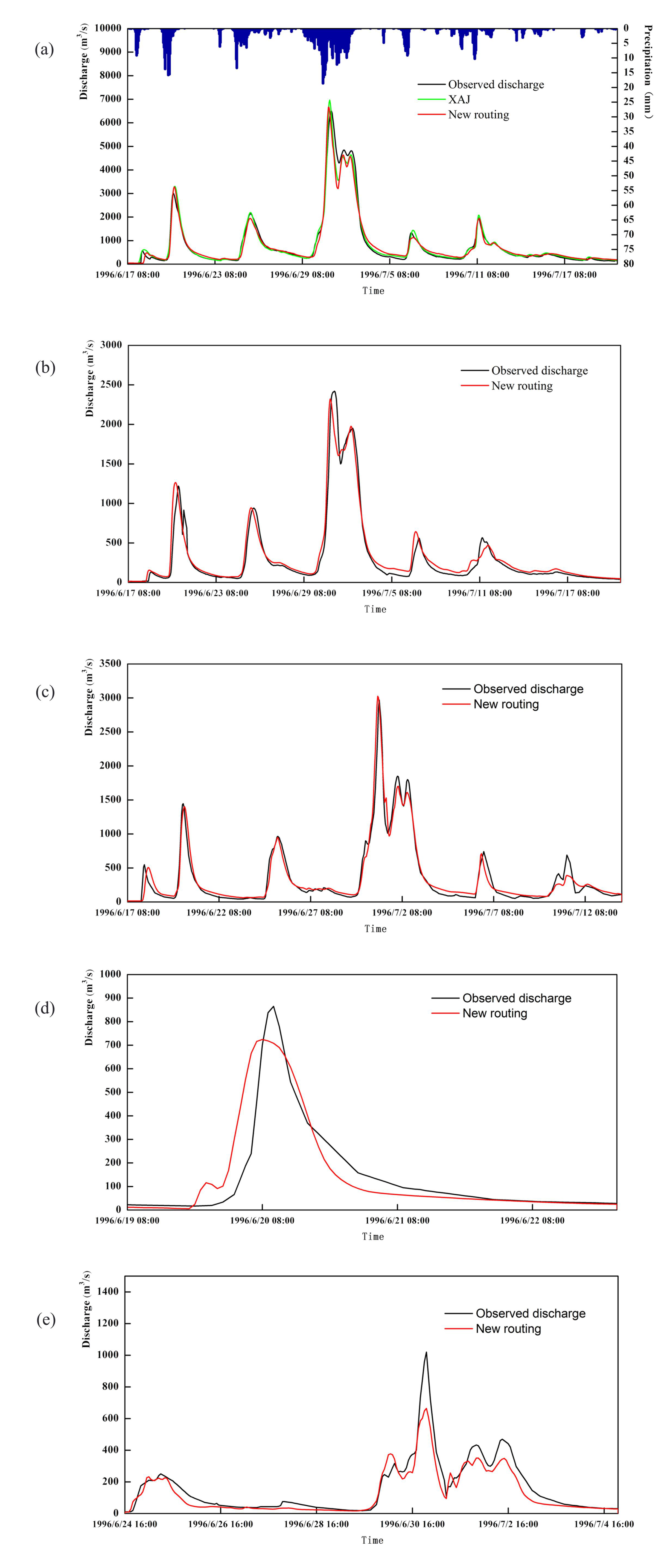
The peak time simulated by the improved model was generally earlier than that by the original Xin’anjiang model. Flood hydrographs simulated by the new routing method tended to steep rising and falling limbs and the simulated peak time was also slightly ahead of the observed peak time according to Figure 7. The peak time of Tunxi simulated by Xin’anjiang model was advanced by 2 h, and that of Tunxi, Yuetan, Wan’an, Chengcun and Xinting simulated by the improved model were advanced by 4, 6, 2, 2 and 1 respectively (Figure 7). It showed the larger the drainage area, the earlier the peak time. According to Figure 6c, it can also be seen that the PTE of the original Xin’anjiang model at outlet Tunxi was concentrated in −5 to 9 h, while the PTE simulated by the improved model at outlet Tunxi ranged from −6 to 4 h. It indicated the peak time of simulations by new runoff routing scheme was slightly earlier than that by original runoff routing scheme.
4.4. Discussion
This paper presents a new runoff routing scheme and couples it with the Xin’anjiang model, in which the isochrone method is employed for overland routing and the grid-to-grid MCT method is employed for main channel routing. What is more, based on the geographic information of the watershed, we establish a set of parameters estimation methods for the new runoff routing scheme. By comparing the results from simulations by new and original runoff routing schemes, we find the performance of the original and new runoff routing models are generally comparable and satisfactory. Furthermore, the new model is able to produce promising simulations for four interior points where no recalibration was done. It also proves that the parameter estimation method is effective.
The results also show simulations by new routing scheme for the location with larger drainage area have higher mean NSE and qualified ratio of RPE. However, simulations for Yuetan and Wanan with the larger drainage area did not outperform simulations for Chengcun. A similar conclusion was reached by Yao (2012) [20]. The main reason may be that spatial variation of rainfall has not been considered enough. The spatial variation of rainfall may not have been accurately captured on account of the fact that the density of rain gauges is low. The rain gauge densities for Yuetan, Wanan and Chengcun are 1 station in 238, 216 and 97 km2, respectively, so spatial variation of rainfall can be more accurately captured at Chengcun (Table 4). These results imply that the spatial rainfall pattern influences the predictions of interior hydrologic processes using parameters only calibrated for the parent watershed.
In addition, we can see from the flood hydrograph shown in Figure 7 that there is still a little defect in the new runoff routing scheme. In this example, flood hydrographs simulated by the new routing method tend to steep rising and falling limbs and the simulated peak time is also slightly ahead of the observed peak time. In particular, the larger the drainage area, the more ahead of peak time. The main reason for this error may be that constant flow velocity and lack of the consideration of river network routing. The second possible cause is that the geometry of the channel is assumed to be rectangular and the width of the river is calculated according to the empirical formula of the river width, which may not be consistent with the actual situation. The third reason may be the spatial parameter variability is not adequately captured in this case, especially overland Manning’s roughness coefficients, which has a significant influence on the flood process.
5. Conclusions
This paper presents a new runoff routing scheme and coupled it with the Xin’anjiang model, in which the isochrone method is employed for overland routing and grid-to-grid MCT method is employed for main channel routing. What’s more, based on the geographic information of the watershed, we establish a set of parameters estimation methods for the new runoff routing scheme. Compared with the original Xin’anjiang model, the advantage of the improved model is that it can predict the flow for internal stations, and its routing parameters can be determined according to geographic information. In this scheme, the length of routing path from each grid flow to the main river channel is determined by DEM based on D8 principle. The flow velocity of overland is mainly determined by land cover types and average slope. Hence, we can determine the lag time of each grid droplet arriving at the main channel. The lag time histogram is employed to determine the percentage of the overland flow arrived at the river channel for each sub catchment at each time step. After using MCT method instead of Muskingum method, the parameters of the model can also be estimated according to river order, channel geometry and channel gradient. This makes the runoff routing scheme established in this paper can be used only with DEM and a multiplier on overland Manning’s roughness . The strengths of our new routing scheme have been demonstrated through its applications to the Tunxi catchment with four interior stations. This approach is a powerful tool for linking the hydrologic response of catchments to their geomorphologic characteristics, which can provide an insight to the hydrologic behavior of ungauged catchments.
Although tests performed in this study with observed data have shown the potential of the new routing scheme model, two additional issues need further research to improve the prediction accuracy of the new runoff routing model.
(1) The problems of steep rising and falling limbs hydrographs and early peak time caused by the traditional isochrone method, due to constant flow velocity and lack of the consideration of river network routing, can be significantly reduced by the new routing scheme. In the future study, other flow velocity formula such as Manning’s formula can be considered to replace the overland velocity formula in this paper for overland routing, so that the average overland velocity changes with time. In addition, the regulation and storage capacity of river network still needs to be further addressed.
(2) With the changes of underlying surface conditions affected by human activities and climate change, land cover types are constantly evolving. Therefore, in the case of land cover and land use change, the fixed model parameter values are not always applicable. Improving the quality of input data (precipitation, land cover, soil type and channel basic information, etc.) is beneficial to increase the accuracy of flood simulation and forecasting. It is anticipated that a new efficient methodology that utilizes appropriate survey information, topographic maps and remote sensing data will be employed in further applications of the model.
Author Contributions
Conceptualization, S.Z. and Z.L.; data curation, S.Z. and Z.L.; formal analysis, S.Z., Z.L. and M.S.; funding acquisition, S.Z., Z.L. and C.Y.; investigation, S.Z., Z.L., K.Z. and C.Y; methodology, S.Z.; project administration, Z.L., C.Y. and K.Z.; resources, S.Z. and Z.L.; software, S.Z. and Z.L.; supervision, Z.L. and C.Y; validation, S.Z., Z.L. and M.S.; visualization, S.Z.; writing—original draft preparation, S.Z.; writing—review and editing, S.Z., Z.L., C.Y., K.Z., M.S. and X.K. All authors have read and agreed to the published version of the manuscript.
Funding
This study was supported by the National Natural Science Foundation of China (Grant No. 51679061) and the National Key Research and Development Program of China (Grant, 2018YFC1508101).
Conflicts of Interest
The authors declare no conflict of interests regarding the publication of this paper.
References
- Smith, M.B.; Laurine, D.P.; Koren, V.; Reed, S.; Zhang, Z. Hydrologic Model. Calibration in the National Weather Service; American Geophysical Union (AGU): Washington, DC, USA, 2003; Volume 6, pp. 133–152. [Google Scholar]
- Gupta, H.V.; Sorooshian, S.; Hogue, T.S.; Boyle, D.P. Advances in Automatic Calibration of Watershed Models; American Geophysical Union (AGU): Washington, DC, USA, 2003; Volume 6, pp. 9–28. [Google Scholar]
- Seyfried, M.S.; Wilcox, B.P. Scale and the Nature of Spatial Variability: Field Examples Having Implications for Hydrologic Modeling. Water Resour. Res. 1995, 31, 173–184. [Google Scholar] [CrossRef]
- Koren, V.; Reed, S.; Smith, M.; Zhang, Z.; Seo, D.-J. Hydrology laboratory research modeling system (HL-RMS) of the US national weather service. J. Hydrol. 2004, 291, 297–318. [Google Scholar] [CrossRef] [Green Version]
- Beven, K. Changing ideas in hydrology—The case of physically-based models. J. Hydrol. 1989, 105, 157–172. [Google Scholar] [CrossRef]
- Wilcox, B.P.; Rawls, W.J.; Brakensiek, D.L.; Wight, J.R. Predicting runoff from Rangeland Catchments: A comparison of two models. Water Resour. Res. 1990, 26, 2401–2410. [Google Scholar] [CrossRef]
- Loague, K. R-5 revisited: 2. Reevaluation of a quasi-physically based rainfall-runoff model with supplemental information. Water Resource. Res. 1990, 26, 973–987. [Google Scholar] [CrossRef]
- Robinson, J.S.; Sivapalan, M. Catchment-scale runoff generation model by aggregation and similarity analyses. Hydrol. Process. 1995, 9, 555–574. [Google Scholar] [CrossRef]
- Chao, L.; Zhang, K.; Li, Z.; Wang, J.; Yao, C.; Li, Q. Applicability assessment of the CASCade Two Dimensional SEDiment (CASC2D-SED) distributed hydrological model for flood forecasting across four typical medium and small watersheds in China. J. Flood Risk Manag. 2019, 12. [Google Scholar] [CrossRef] [Green Version]
- Reed, S.; Koren, V.; Smith, M.; Zhang, Z.; Moreda, F.; Seo, D.-J.; Participants, A.D. Overall distributed model intercomparison project results. J. Hydrol. 2004, 298, 27–60. [Google Scholar] [CrossRef]
- Moore, R.J.; Cole, S.J.; Bell, V.A.; Jones, D.A. Issues in Flood Forecasting: Ungauged Basins, Extreme Floods and Uncertainty. In Frontiers in Flood Forecasting, Eighth Kovacs Colloquium, June/July 2006, UNESCO, Paris; Tchiguuirinskaia, I., Thein, K.N.N., Hubert, P., Eds.; IAHS Publication: Wallingford, Oxfordshire, UK, 2006; pp. 103–122. [Google Scholar]
- WMO. Manual on Flood Forecasting and Warning. World Meteorological Organization; WMO: Geneva, Switzerland, 2011; p. 1072. [Google Scholar]
- Liu, Y.; Zhang, K.; Li, Z.; Liu, Z.; Wang, J.; Huang, P. A hybrid runoff generation modelling framework based on spatial combination of three runoff generation schemes for semi-humid and semi-arid watersheds. J. Hydrol. 2020, 590. [Google Scholar] [CrossRef]
- Ren-Jun, Z. The Xinanjiang model applied in China. J. Hydrol. 1992, 135, 371–381. [Google Scholar] [CrossRef]
- Zhao, R. Watershed concentration flow of linear time-varying systems. J. China Hydrol. 1991, 4, 22–24. [Google Scholar]
- Xu, Q.; Li, Z.; Chen, X. Study on the parameter laws of watershed flow concentration of Xinanjiang model. Boutiq. China Sci. Technol. Papers Online 2008, 2, 335–338. [Google Scholar]
- Hu, W.; Li, Z.; Zhang, H.; Zhong, L. Study on relationship between recession coefficient of river network and underlying surface for Xin’ anjiang model. Water Resource. Power 2017, 35, 14–17. [Google Scholar]
- McCarthy, G.T. The Unit Hydrograph and Flood Routing. In Proceedings of the Proceedings of Conference of North Atlantic Division, US Army Corps of Engineers, New London, CT, USA, 24 June 1938. [Google Scholar]
- Yao, C.; Li, Z.; Bao, H.; Yu, Z. Application of a developed Grid-Xin’anjiang model to Chinese watersheds for flood forecasting purpose. J. Hydrol. Eng. 2009, 14, 923–934. [Google Scholar] [CrossRef]
- Yao, C.; Li, Z.; Yu, Z.; Zhang, K. A priori parameter estimates for a distributed, grid-based Xinanjiang model using geographically based information. J. Hydrol. 2012, 468, 47–62. [Google Scholar] [CrossRef]
- Yao, C.; Zhang, K.; Yu, Z.; Li, Z.; Li, Q. Improving the flood prediction capability of the Xinanjiang model in ungauged nested catchments by coupling it with the geomorphologic instantaneous unit hydrograph. J. Hydrol. 2014, 517, 1035–1048. [Google Scholar] [CrossRef]
- Beven, K. Rainfall-Runoff Modelling: The Primer, the Seconded; John Wiley & Sons, Ltd.: Hoboken, NJ, USA, 2012. [Google Scholar]
- Saghafian, B.; Julien, P.Y.; Rajaie, H. Runoff hydrograph simulation based on time variable isochrone technique. J. Hydrol. 2002, 261, 193–203. [Google Scholar] [CrossRef]
- Wen, Z.; Liang, X.; Yang, S. A new multiscale routing framework and its evaluation for land surface modeling applications. Water Resour. Res. 2012, 48. [Google Scholar] [CrossRef]
- Todini, E. A Mass Conservative and Water Storage Consistent Variable Parameter Muskingum-Cunge Approach. Hydrol. Earth Syst. Sci. 2007, 4, 1645–1659. [Google Scholar] [CrossRef] [Green Version]
- Liu, Z.; Todini, E. Towards a comprehensive physically-based rainfall-runoff model. Hydrol. Earth Syst. Sci. 2002, 6, 859–881. [Google Scholar] [CrossRef]
- Rodríguez-Iturbe, I.; Valdés, J.B. The geomorphologic structure of hydrologic response. Water Resour. Res. 1979, 15, 1409–1420. [Google Scholar] [CrossRef] [Green Version]
- Rui, X. Study of determining geomorphologic unit hydrograph by means of probability density functions of path length and slope. Adv. Water Sci. 2003, 14, 602–606. [Google Scholar]
- Xiaofang, R.; Mei, Y.; Fanggui, L.; Xinglong, G. Calculation of watershed flow concentration based on the grid drop concept. Water Sci. Eng. 2008, 1, 1–9. [Google Scholar] [CrossRef] [Green Version]
- Gupta, V.K.; Waymire, E.; Wang, C.T. A representation of an instantaneous unit hydrograph from geomorphology. Water Resour. Res. 1980, 16, 855–862. [Google Scholar] [CrossRef]
- O’Callaghan, J.; Mark, D.M. The extraction of drainage networks from digital elevation data. Comput. Vision Graph. Image Process. 1984, 27, 247. [Google Scholar] [CrossRef]
- Graham, S.T.; Famiglietti, J.S.; Maidment, D.R. Five-minute, 1/2°, and 1° data sets of continental watersheds and river networks for use in regional and global hydrologic and climate system modeling studies. Water Resour. Res. 1999, 35, 583–587. [Google Scholar] [CrossRef] [Green Version]
- Oki, T.; Sud, Y.C. Design of Total Runoff Integrating Pathways (TRIP)—A Global River Channel Network. Earth Interact. 1998, 2, 1–37. [Google Scholar] [CrossRef]
- Wang, M.H.; Hjelmfelt, A.T.; Garbrecht, J. DEM aggregation for watershed modeling. Jawra J. American Water Resource. Assoc. 2010, 36, 579–584. [Google Scholar] [CrossRef]
- Lohmann, D.; Nolte-Holube, R.; Raschke, E. A Large-Scale Horizontal Routing Model to be Coupled to Land Surface Parametrization Schemes. Tellus Ser. A 1996, 48, 708–721. [Google Scholar] [CrossRef]
- Reggiani, P.; Todini, E.; Meißner, D. A conservative flow routing formulation: Déjà vu and the variable-parameter Muskingum method revisited. J. Hydrol. 2014, 519, 1506–1515. [Google Scholar] [CrossRef]
- Gochis, D.J.; Barlage, M.; Dugger, A.; FitzGerald, K.; Karsten, L.; McAllister, M.; McCreight, J.; Mills, J.; RafieeiNasab, A.; Read, L.; et al. The WRF-Hydro Modeling System Technical Description (Version 5.0); Center for Atmospheric Research (NCAR): Boulder, CO, USA, 2018; Available online: http://ral.ucar.edu/sites/default/files/public/WRFHydroV5TechnicalDescription.pdf (accessed on 13 April 2018).
- MWR. Standard for Hydrological Information and Hydrological Forecasting (GB/T 2482-2008); Ministry of Water Resources of the People’s Republic of China, Standards Press of China, Beijing: Beijing, China, 2008; p. 16.
- Nash, J.E.; Sutcliffe, J.V. River flow forecasting through conceptual models part I—A discussion of principles. J. Hydrol. 1970, 10, 282–290. [Google Scholar] [CrossRef]
Figure 1.
Structural chart of Xin’anjiang model and the new runoff routing scheme.

Figure 2.
The histograms of the overland flow path lengths.

Figure 3.
Map for the study catchments and locations of the rain gauges.

Figure 4.
Land cover type maps for Tunxi catchment.

Figure 5.
Relationship between river width and upstream drainage area in Tunxi catchment.

Figure 6.
Box plots of the relative runoff volume error (RRE), relative peak discharge error (RPE), peak time error (PTE) and Nash–Sutcliffe efficiency (NSE) statistics of all events by the original Xin’anjiang model (XAJ) and the new routing scheme at the catchment outlet TX and interior locations Yuetan (YT), Wanan (WA), Chengcun (CC) and Xinting (XT).

Figure 7.
Examples of simulated and observed hydrographs for the Tunxi watershed by the original Xin’anjiang model (XAJ) and the improved model (new routing) at the catchment outlet (a) Tunxi and interior locations (b) Yuetan, (c) Wanan, (d) Chengcun and (e) Xinting.
Figure 7.
Examples of simulated and observed hydrographs for the Tunxi watershed by the original Xin’anjiang model (XAJ) and the improved model (new routing) at the catchment outlet (a) Tunxi and interior locations (b) Yuetan, (c) Wanan, (d) Chengcun and (e) Xinting.


Table 1.
Data records of the study catchments.
| Station Name | Period for Flood Events | Number of Flood Events |
|---|---|---|
| Tunxi (TX) | 1982–2003 | 33 |
| Yuetan (YT) | 1982–2003 | 33 |
| Wanan (WA) | 1988–2003 | 22 |
| Chengcun (CC) | 1986–1999 | 25 |
| Xinting (XT) | 1986–2000 | 27 |
Table 2.
List of calibrated parameters of the Xin’anjiang model.
| Parameter | Description | Parameter Values |
|---|---|---|
| Ke | Ratio of potential evapotranspiration to pan evaporation | 1.08 |
| Wum | Tension water capacity of upper layer (mm) | 20 |
| Wlm | Tension water capacity of lower layer (mm) | 73 |
| C | Evapotranspiration coefficient of deeper layer | 0.08 |
| B | Exponent of distribution of tension water capacity | 0.532 |
| Wm | Tension water capacity (mm) | 120 |
| Im | Ratio of impervious area to the total area of the catchment | 0.0014 |
| Sm | Free water capacity (mm) | 20 |
| Ex | Exponent of distribution of free water capacity (mm) | 1.2 |
| Kg | Outflow coefficient of free water storage to groundwater | 0.35 |
| Ki | Outflow coefficient of free water storage to interflow | 0.35 |
| Cg | Recession constant of groundwater storage | 0.998 |
| Ci | Recession constant of interflow storage | 0.87 |
| CS | Recession constant in the lag-and-route method | 0.9 |
| Lag | Lag time (h) | 2 |
| Muskingum time constant for each sub-reach (h) | 1 | |
| Muskingum weighting factor for each sub-reach | 0.35 |
Table 3.
Manning’s roughness coefficient values and overland slopes of Tunxi sub catchments.
| Sub Catchments | Overland Roughness | Overland Slope | Channel Roughness |
|---|---|---|---|
| Wucheng (WC) | 0.1275 | 0.015984 | 0.025 |
| Shimen (SM) | 0.1275 | 0.031171 | 0.025 |
| Zuolong (ZL) | 0.1275 | 0.035772 | 0.025 |
| Dalian (DL) | 0.1275 | 0.033066 | 0.025 |
| Tunxi (TX) | 0.055 | 0.023073 | 0.018 |
| Shangxikou (SXK) | 0.2 | 0.023417 | 0.025 |
| Rucun (RC) | 0.1275 | 0.028201 | 0.018 |
| Yixian (YX) | 0.1275 | 0.010486 | 0.018 |
| Yanqian (YQ) | 0.1275 | 0.024971 | 0.018 |
| Xiuning (XN) | 0.03 | 0.079677 | 0.018 |
| Chengcun (CC) | 0.1275 | 0.125944 | 0.025 |
Table 4.
Accuracy statistics of the improved model simulations for both calibration and validations events.
Table 4.
Accuracy statistics of the improved model simulations for both calibration and validations events.
| Station Name | Rain Gauges | Drainage Area (Km2) | Rain Gauges Network Intensity (/Km2) | Qualified Ratio (%) | Average | ||
|---|---|---|---|---|---|---|---|
| RRE | RPE | PTE | NSE | ||||
| Tunxi (TX) | 11 | 2692 | 245 | 100 | 81.3 | 81.3 | 0.92 |
| Yuetan (YT) | 4 | 952 | 238 | 87.9 | 81.8 | 66.7 | 0.88 |
| Wanan (WA) | 4 | 865 | 216 | 63.6 | 72.7 | 86.4 | 0.85 |
| Chengcun (CC) | 3 | 290 | 97 | 88.0 | 88.0 | 96.0 | 0.86 |
| Xinting (XT) | 1 | 184 | 184 | 92.6 | 65.0 | 88.9 | 0.84 |
Publisher’s Note: MDPI stays neutral with regard to jurisdictional claims in published maps and institutional affiliations. |
© 2020 by the authors. Licensee MDPI, Basel, Switzerland. This article is an open access article distributed under the terms and conditions of the Creative Commons Attribution (CC BY) license (http://creativecommons.org/licenses/by/4.0/).
Share and Cite
MDPI and ACS Style
Zang, S.; Li, Z.; Yao, C.; Zhang, K.; Sun, M.; Kong, X. A New Runoff Routing Scheme for Xin’anjiang Model and Its Routing Parameters Estimation Based on Geographical Information. Water 2020, 12, 3429. https://doi.org/10.3390/w12123429
AMA Style
Zang S, Li Z, Yao C, Zhang K, Sun M, Kong X. A New Runoff Routing Scheme for Xin’anjiang Model and Its Routing Parameters Estimation Based on Geographical Information. Water. 2020; 12(12):3429. https://doi.org/10.3390/w12123429
Chicago/Turabian StyleZang, Shuaihong, Zhijia Li, Cheng Yao, Ke Zhang, Mingkun Sun, and Xiangyi Kong. 2020. "A New Runoff Routing Scheme for Xin’anjiang Model and Its Routing Parameters Estimation Based on Geographical Information" Water 12, no. 12: 3429. https://doi.org/10.3390/w12123429
Note that from the first issue of 2016, this journal uses article numbers instead of page numbers. See further details here.