Impact of Water Deficit on Seasonal and Diurnal Dynamics of European Beech Transpiration and Time-Lag Effect between Stand Transpiration and Environmental Drivers

Abstract

In-situ measurements of tree sap flow enable the analysis of derived forest transpiration and also the water state of the entire ecosystem. The process of water transport (by sap flow) and transpiration through vegetation organisms are strongly influenced by the synergistic effect of numerous external factors, some of which are predicted to alter due to climate change. The study was carried out by in-situ monitoring sap flow and related environmental factors in the years 2014 and 2015 on a research plot in Bienska dolina (Slovakia). We evaluated the relationship between derived transpiration of the adult beech (Fagus sylvatica L.) forest stand, environmental conditions, and soil water deficit. Seasonal beech transpiration (from May to September) achieved 59% of potential evapotranspiration (PET) in 2014 and 46% in 2015. Our study confirmed that soil water deficit leads to a radical limitation of transpiration and fundamentally affects the relationship between transpiration and environmental drivers. The ratio of transpiration (E) against PET was significantly affected by a deficit of soil water and in dry September 2015 decreased to the value of 0.2. The maximum monthly value (0.8) of E/PET was recorded in August and September 2014. It was demonstrated that a time lag exists between the course of transpiration and environmental factors on a diurnal basis. An application of the time lags within the analysis increased the strength of the association between transpiration and the variables. However, the length of these time lags changed in conditions of soil drought (on average by 25 min). Transpiration is driven by energy income and connected evaporative demand, provided a sufficient amount of extractable soil water. A multiple regression model constructed from measured global radiation (R_S), air temperature (AT), and air humidity (RH) explained 69% of the variability in beech stand transpiration (entire season), whereas (R_S) was the primary driving force. The same factors that were shifted in time explained 73% of the transpiration variability. Cross-correlation analysis of data measured in time without water deficit demonstrated a tighter dependency of transpiration (E) on environmental drivers shifted in time (−60 min R_S, +40 min RH and +20 min vapour pressure deficit against E). Due to an occurrence and duration of soil water stress, the dependence of transpiration on the environmental variables became weaker, and at the same time, the time lags were prolonged. Hence, the course of transpiration lagged behind the course of global radiation by 60 (R² = 0.76) and 80 (R² = 0.69) minutes in conditions without and with water deficit, respectively.

1. Introduction

Plant transpiration is a major component of terrestrial ecosystem evapotranspiration and represents a significant water loss term of the water balance [1]. In terrestrial conditions, 39% of precipitation returns to the atmosphere through transpiration, which accounts for 61% of evapotranspiration, on average. Besides, forest ecosystem transpiration can contribute 50–70% of terrestrial evapotranspiration [2]. Therefore, most water evaporating from ecosystems transits through plant organisms and its concrete volume is regulated by plants [3]. At the same time, evapotranspiration can account for over 50% of the total water loss in most terrestrial ecosystems and belongs to the primary water-loss components of the water cycle [4,5].

Evapotranspiration can be estimated relatively precisely, but it requires a high investment in equipment, well-trained research personnel and know-how [6]. The methods of direct measurement of evapotranspiration are currently rather limited, particularly in woody crops [6,7]. However, transpiration can be estimated utilising sap flow monitoring. The physiological process of transpiration and water flux through xylem are well known. In recent years, several methods for the precise measurement of tree trunk sap flow have been developed and successfully applied in research [8,9]. Modern systems are relatively affordable, undemanding to use, and some provide instant information on sap flow without demanding recalculations [10]. Hence, at a larger time scale (i.e., days and longer), the amount of water flow through the trunk is approximately equal to canopy transpiration [11]. Therefore, the monitoring of sap flow is a highly useful tool to observe and investigate the impact of environmental conditions, including extreme events such as drought, on forest water balance and its stress load [12,13]. Sap flow measurements have become a standard tool for ecosystem research [14].

A detailed study of transpiration, its limitations, and the dynamics in connection to changing environmental conditions is important for understanding the impact of vegetation on hydrology and can help improve ecosystem water balance modelling and to predict plant responses to climate change [1,9,15,16]. Transpiration is influenced by the synergic effect of environmental factors, vegetation characteristics (leaf area index (LAI), tree age and vitality, stocking density, root system) and management (thinning, pruning) [17]. The impact of environmental factors is significant and can be divided into atmospheric evaporative demands (potential evapotranspiration and vapour pressure deficit) [16,18] and soil moisture, the lack of which leads to limited plant transpiration [19,20,21]. However, some woody species can uptake water even from groundwater or bedrock fractures [22,23]. Environmental factors are predicted to change in connection to human-induced global warming, which according to the IPCC report, reached approximately 1 °C (likely between 0.8 °C and 1.2 °C) above pre-industrial levels in 2017, increasing at 0.2 °C per decade (high confidence) [24]. Various climate scenarios predict a substantial change in precipitation distribution and in average temperatures, which can cause more prolonged and severe summer drought [25,26]. A warmer atmosphere means increased evaporation demands and is accompanied by a lack of water supply, leading to an intensification of water-related plant stress [27,28]. Water deficit results in drought stress, substantially limiting the physiological processes of plants and phytomass formation and may result in a long-term decrease in forest productivity [29,30] and an increase in drought-induced mortality [31,32,33].

As aforementioned, the main weather parameters that affect transpiration, together with crop characteristics and water supply, are radiation, air temperature, humidity, and wind speed. A common effect of these parameters can be expressed via the evaporation power of the atmosphere (potential evapotranspiration or reference crop evapotranspiration) [34]. Over the years, several research papers have been published focused on modelling the water use (transpiration or sap flow) of various tree species [3,35,36,37,38]. The simulation of tree water use is carried out using several environmental variables applying various approaches [38]. Some studies point out that within the relationship between sap flow (or transpiration) and environmental variables exists a time lag of varying range and direction [3,39,40,41]. This time lag is the main characteristic of the hysteresis phenomenon, which was detected and described in many studies within different species and ecosystems [40,42,43]. Overall, the diurnal course of sap flow can lag behind the course of the environmental driver or can occur in advance. The time lag between measured sap flow and environmental factors can be caused by the priority use of trunk water storage for transpiration, particularly in the morning [40,44]. At the same time, hysteresis is considered to be a conservation mechanism to prevent dehydration during high evaporative demand [45]. However, prior studies demonstrated that time lags were affected by drought, solar radiation, and high evaporation demands [42,46]. The study of these time lags can advance our understanding and, therefore, improve the response of vegetation to changing climate factors, and the inclusion of the detected lags can enhance water flux modelling [40,41].

Our study focused on assessing the seasonal and diurnal dynamics of sap flow-derived transpiration of mature beech stand in relation to changing environmental drivers with an emphasis on the occurrence of drought. European beech (Fagus sylvatica L.) belongs to the essential broadleaved species in Europe, from both an economic and ecological point of view [30,47]. Beech increases the stability of forest stands, which is reflected in its pan-European application in the silvicultural concepts of reconstructing non-natural monocultural conifer stands (mostly spruce) to stable and resilient mixed forests more resistant to predicted climate change [48,49,50]. On the other hand, beech decline in Europe was reported in connection with a drought-related decrease in tree vitality, which causes subsequent increased endanger due to biotic factors, such as insects and wood decay fungi [51,52,53].

In Slovakia, European beech, with a share of almost 34% (with an increasing trend), is the most commonly occurring tree species and has the largest share of wood production within deciduous tree species [50]. Beech forests, due to their broad areas of spread, significantly contribute to the hydrological cycle by water transpiration and interception, with transpiration having the largest share regarding beech stand total evapotranspiration [54]. In the context of climate change, it is predicted that beech ecosystems will be threatened all over Europe [55] and will be exposed to severe stress from drought because shallow-rooting beech is considered a drought-sensitive species [47,56,57]. Drought episodes and increased temperature during the growing season negatively affect beech stands’ water balance, growth, competitiveness, and resilience. The effect is increased during the prolonged duration of the dry season and has been repeated for several years in a row [47,57,58,59]. The limitation in beech growth as a consequence of drought and resulting reduced tree competitiveness was documented already in the 20th century [60]. Similarly, recent research results confirm a 17% reduction of annual gross primary beech production due to the 2003 drought [61]. A study from 2019 concluded that the European beech is, in particular, sensitive to a lack of precipitation and is less sensitive to heat stress [61].

The main objectives of this study were, therefore, to (i) describe the seasonal and diurnal dynamics of beech transpiration in relation to the course of environmental factors affecting transpiration, focusing on the drought effect, (ii) detect the time lags between the transpiration and meteorological drivers, and (iii) assess the impact of water deficit on time lags.

2. Materials and Methods

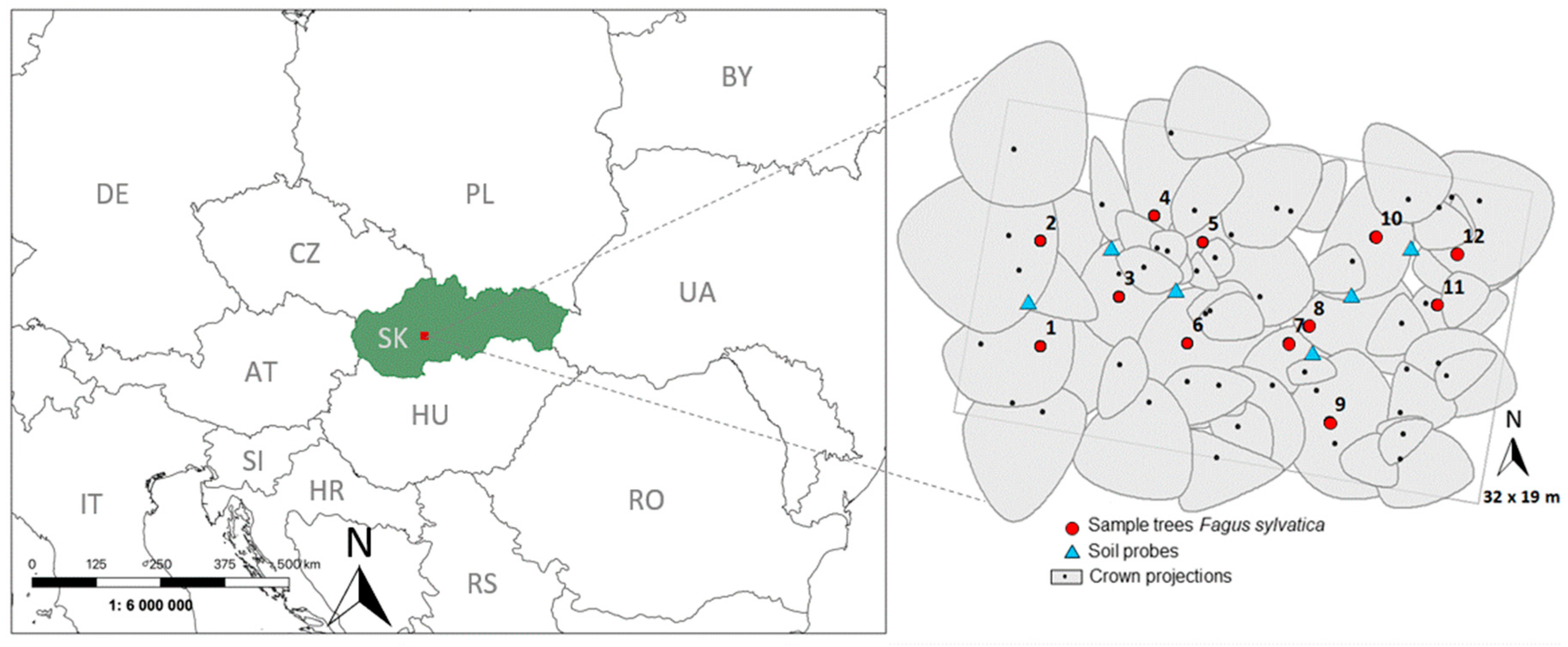
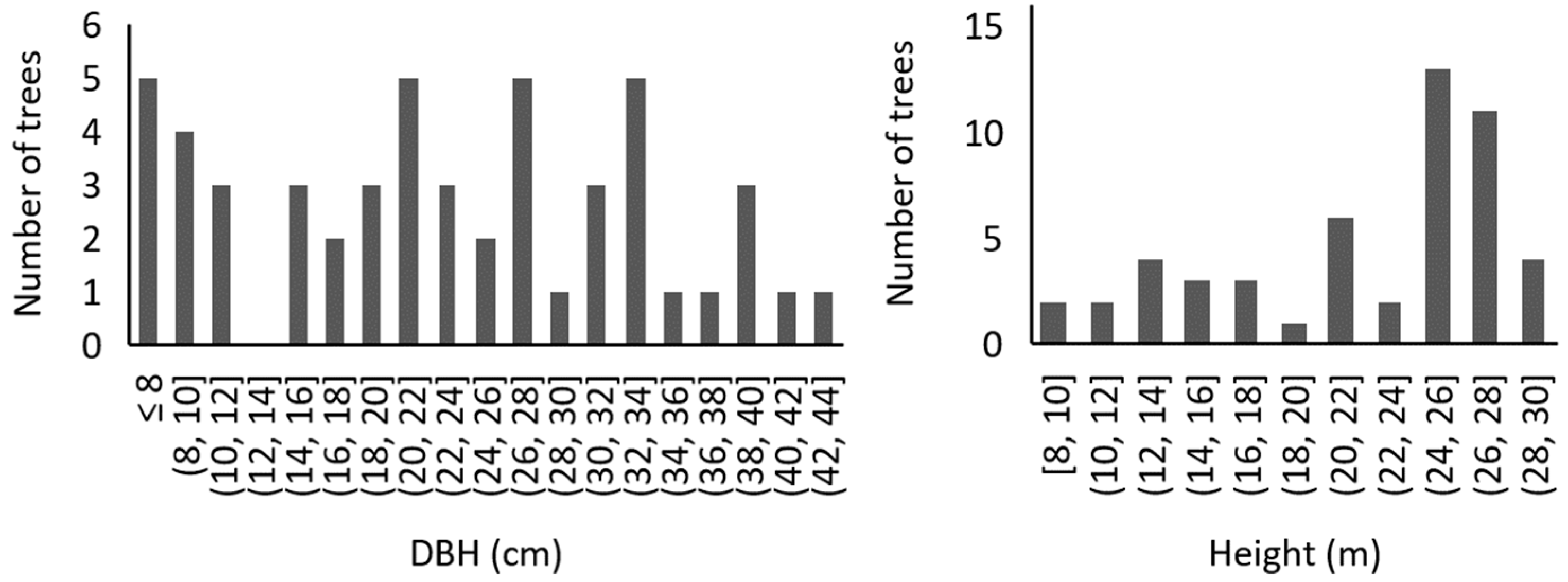
2.1. Experimental Stand

The study was conducted in the area of Bienska dolina, situated in the central part of the Slovak Republic at an elevation of 450 m a.s.l. with coordinates 48°36′43″ N and 19°03′59″ E (Figure 1). The locality is classified as a 3rd oak-beech altitudinal forest zone (classification according to Zlatník [62]) with Haplic Cambisol (Humic, Eutric, Endoskeletic, and Siltic) formed on volcanic parent material (andesite and andesitic tuffs) [63]. The depth of soil reaches a maximal 66 cm. The textural class of the fine-earth fraction is detected as silt loam in the topsoil or loam in the subsoil. Upper horizons are characterised by the presence of only a small amount of coarse rock fragments, whereas coarse gravel and stones are plentiful in the subsoil (C horizon, up to 80%). The abundance of roots in the upper 30–35 cm of soil is relatively high and decreases in deeper soil layers.

An experimental plot with an area of 608 m² was established in a 68-year-old European beech forest, which is dominated by Fagus sylvatica L. with a minor admixture of Quercus petraea (Matt.) Liebl. (sessile oak, 10%) and Larix decidua (Mill.) (larch, 5%). However, these admixture species occur outside the delineated plot. The slope is east facing and, on average reaches a maximum of 30%. The relative stocking density of the stand is 0.85 with a maximum leaf area index of 6.1 in July (LAI-2200 Plant Canopy Analyzer, LI-COR Biosciences, Lincoln, NE, USA). The total stand volume of beech is 282 m³ ha⁻¹. The understory vegetation is poor and is characterised by the rare occurrence of beech seedlings and typical herbs species, such as Asarum europaeum and Dentaria bulbifera.

Within the area of the experimental plot (608 m²), 56 trees were measured using Field-Map technology, which combines real-time GIS software with electronic equipment for mapping and dendrometric measurements (IFER Ltd., Jílové u Prahy, Czech Republic). Using this technology, the main dendrometric characteristics (tree height, diameter at breast height (DBH) and crown projection) of trees were focused upon and documented (Figure 1, right). The measured DBH of beech trees at the plot varied from 5.7 to 42.3 cm, and heights were from 8.4 to 29.3 m. The distribution of trees within the DBH classes is presented in Figure 2. From these trees, 12 representative sample trees were chosen based on DBH, height and their location to apply sap flow measurement systems. Sample trees were characterised by a mean tree height of 26.3 m ± 1.3 m (from 24.7 to 29.1 m) and an average diameter (DBH) of 32.4 cm ± 4.8 cm (from 27.1 to 42.3 cm).

The climate of Bienska dolina is classified as slightly warm and moderately humid [64]. Figure 3 shows the 1961–1990 reference period’s monthly averages (normals) of mean air temperature (AT) and precipitation totals (P) for the area, calculated based on data from a nearby station belonging to a network of professional meteorological stations of the Slovak Hydrometeorological Institute. The long-term mean annual air temperature and annual sum of precipitation are 7.3 °C and 690 mm, respectively. The normal values during the vegetation season (May–September) are 14.8 °C for mean temperature and 250 mm for precipitation. The rainiest month according to the reference period is June, with an average precipitation of 90 mm, and the warmest month is July, with an average temperature of 17 °C.

2.2. Measured and Derived Environmental Variables

Meteorological variables were during the years 2014 and 2015 measured within an open grass area situated ca. 250 m from the experimental stand by an automatic meteorological station. The station was equipped with an air temperature (AT, °C) and relative humidity (RH, %) sensor and a global radiation (R_S, W m⁻²) sensor (EMS33 and EMS11; Environmental Measuring System (EMS Brno) Ltd., Brno, Czech Republic), which were situated at a height of 2 m above ground (low cut grass). Wind speed (u, m s⁻¹) was monitored using a 034B Wind Sensor (Met One Instruments Inc., Grants Pass, OR, USA) at a height of 2 m, and precipitation (P, mm) was measured using a rain gauge type 370 with a collecting area of 320 cm² placed at a height of 1 m above ground (Met One Instruments Inc.). The interval of measurements was 5 min, and data were stored every 20 min in the data logger edgeBox V12 (EMS Brno Ltd.) powered by a 12 V solar-charged battery.

Potential evapotranspiration (PET, mm h⁻¹) as a variable representing theoretical atmospheric evaporative demands unaffected by soil water deficit was calculated according to the Penman equation [65] (Equation (1)).

$$PET=\frac{\mathsf{\Delta }}{\mathsf{\Delta }+\gamma }{R}_n+\frac{\gamma }{\mathsf{\Delta }+\gamma }\frac{6.43 (1+0.536 u) VPD}{\lambda }$$

(1)

where Δ is the slope of the saturation vapour pressure curve (kPa K⁻¹), Rn is the net radiation (W m⁻²) estimated as 77% of the global incoming solar radiation [34] and u is the wind speed measured at 2 m height. The used psychometric constant (γ) was 66 Pa K⁻¹ and the latent heat of vaporization (λ) was 2.45 MJ kg⁻¹ [34].

VPD is the vapour pressure deficit (kPa) calculated by Equation (2).

$$VPD=e_s-e_a$$

(2)

where e_s is the saturated vapour pressure at a given air temperature and e_a is the vapour pressure of the free-flowing air.

Soil water potential (SWP, MPa) was continuously measured using measuring sets containing three calibrated gypsum blocs (Delmhorst Inc., Towaco, NJ, USA), and data were stored at 60-min intervals in a data logger (MicroLog SP3, EMS Brno Ltd., Brno, Czech Republic). SWP values varied from 0 up to –1.5 MPa (the lowest measurable limit of the equipment). Measurements were provided in six different soil profiles distributed across the research plot and were conducted at soil depths of 15, 30, and 50 cm with respect to the depth of soil, which is maximal at 66 cm. In this paper, we used average values of the three depths of the research plot.

Daily relative extractable soil water (REW, dimensionless) at the stand scale was calculated using the forest water balance model BILJOU© (https://appgeodb.nancy.inra.fr/biljou/), a detailed description of which is given in Granier et al. [66]. The model required daily meteorological data (measured wind speed, precipitation, air temperature, relative humidity, global radiation), maximum leaf area index (LAI), and day of the year (DOY) of the onset of phenophase budburst (DOY 105) and leaf fall (DOY 298), maximum extractable soil water (98 mm in the entire root zone), vertical root distribution, and soil properties (determined by soil analysis). REW is widely used to quantify drought intensity and varies between 1 (when the soil is at field capacity) and 0 (permanent wilting point). When REW drops below a critical threshold of 0.4 (REW falls below 40% of maximum extractable water), a soil water deficit is assumed to occur, and transpiration is gradually reduced due to stomatal closure [31,66]. The model calculates REW according to Equation (3).

$$REW=\frac{EW}{E{W}_M}$$

(3)

where EW is the actual extractable soil water in the rooting zone (EW = available soil water–minimum soil water (i.e., lower limit of water availability)), and EW_M is the maximum extractable soil water (EW_M = soil water content at field capacity–minimum soil water (i.e., lower limit of water availability)).

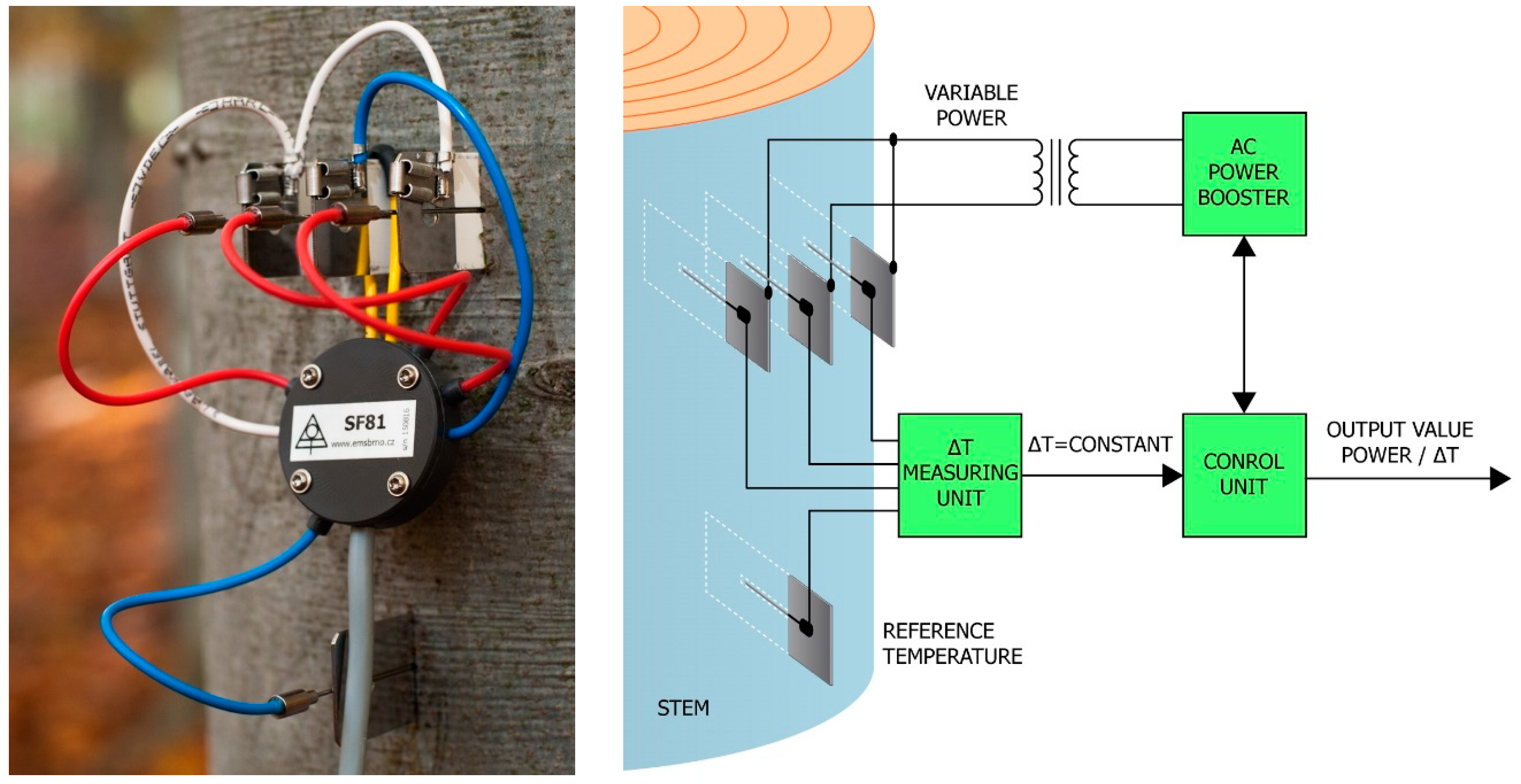
2.3. Sap Flow and Scaling up to Forest Stand Level

On the selected 12 sample trees, at a stem height of ca. 2 m, EMS51A Sap Flow systems connected to a 16-channel datalogger RailBox V16 manufactured by EMS Brno Ltd. (Brno, Czech Republic) were installed. The system uses a tissue heat balance method (THB, [8,67]) based on volume (three-dimensional) heating of the stem segment [10] to measure the values of volumetric sap flow directly in kg of water per a specific period and per one centimetre of stem circumference. The sap flow in Bienska dolina was measured at 5-min intervals and logged as 20-min averages in the datalogger. To obtain sap flow per the entire tree, we recalculated the raw values of sap flow (kg h⁻¹ cm⁻¹) according to the corresponding circumference of the individual sample trees (kg h⁻¹ tree⁻¹). In this paper, we processed the data of sap flow measurements performed during the growing season (from May to end of September) for the years 2014 and 2015.

The system used is designed for large trees with a stem diameter larger than 12 cm, whereas its underlying theory is clear with the absence of uncertain empirical parameters and without the need for field calibration as stated by the manufacturer (http://www.emsbrno.cz/p.axd/en/Sap.Flow.large.trees.html) and Tatarinov et al. [10]. The system consists of a controlling unit (MicroSet8X), sap flow sensor and a set of stainless steel electrodes. The measuring area was protected against direct sunlight and water using reflective insulation. The system (via controlling unit) maintains a pre-set (constant) temperature difference (used value 1 K) between a defined spatial sector of sapwood and reference probes (with an accuracy better than 1%) by electronic control using the variable electric heating power of the controller as the primary signal to quantify sap flux via the heat capacity of water [9]. The sapwood section was internally heated with alternating current (average power consumption 0.3–0.4 W by temperature difference 1 K) by three stainless steel plate electrodes 25-mm wide and 1-mm thick (available in three lengths: 60, 70, and 80 mm). The three electrodes in series plus one reference electrode 10 cm below were inserted at distances exactly 2 cm into the sapwood, passing through the xylem tissues. The central electrode was placed in a radial direction relative to the tree trunk (Figure 4). Into the geometrical centre of these electrodes, the thermosensor needles were inserted to measure temperature differences between the upper and lower electrodes [8,9]. The volume heating method provides a relatively stable temperature field under different values of affected factors (such as wood heat conductivity, sap flow radial profile and temperature gradients), despite this approach requiring relatively higher power consumption [10]. This method eliminates errors in measuring the dynamics of sap flow due to the principle of maintaining a constant temperature for the heated part (no time required to reach steady-state) [10,67].

The general equation that describes the heat balance of xylem takes the following form:

$$P=Q_r dT c_w+dT z$$

(4)

where P is the power of heat input (W), Q_r is the amount of water passing through the heated volume (kg s⁻¹), dT is the temperature difference within the measuring point (K), c_w is the specific heat of water (J kg⁻¹ K⁻¹), and z represents the coefficient heat losses from the measuring point (W K⁻¹).

Water passing through the measuring point (in terms of volume or mass) is calculated from the power input and temperature rise of water passing through the heated space. The sap flow (kg s⁻¹ cm⁻¹) calculation (Equation (5)) is derived from Equation (4).

$$Q=\frac{P}{c_w d dT}-\frac{z}{c_w}$$

(5)

where d is the effective width of the measuring point (5.5 cm), and z/c_w expresses heat losses from the sensor, which is set when Q is equal to zero (P, c_w and dT are listed in the description of Equation (4)) [67,68].

Figure 4. Installed Sap Flow System produced by EMS Brno Ltd. (Brno, Czech Republic) and the flows chart of measuring process. Sap flow values are calculated directly from the P/dT ratio.

Figure 4. Installed Sap Flow System produced by EMS Brno Ltd. (Brno, Czech Republic) and the flows chart of measuring process. Sap flow values are calculated directly from the P/dT ratio.

Based on these measurements, we performed the upscaling from individual tree sap flow to the forest stand on the base of sap flow distribution at the diameter at breast height (DBH; diameter of the tree at a height at 1.3 m) classes [8]. The first step was to obtain the values of sap flow for mean trees (Q_mean, kg h⁻¹) of m DBH classes by means of regression relating the sap flow of the measured sample tree (Q_sample, kg h⁻¹) to the chosen biometric parameter—DBH. These regression analyses were performed with data obtained during a period of constant and sufficient soil water separately for the years 2014 and 2015. Derived Q_mean values were multiplied by numbers of trees in DBH classes (n_i) and then summarised within the stand area unit of 1 ha (Equation (6)). The result represents the sap flow values of the entire forest stand (Q_stand).

$$Q_{stand}={\displaystyle \sum _{i=1}^{i=m}}{\left(Q_{mean}\right)}_i n_i$$

(6)

By dividing gained stand sap flow (Q_stand) by the sum of sap flow directly measured (Q_sample), we determined the non-dimensional coefficient S (-) (Equation (7)). Finally, we multiplied the measured sap flow data (20-min) by the coefficient S and obtained stand-level values, which we considered to be equal to stand transpiration (E, mm h⁻¹ (kg m⁻² h⁻¹)).

$$S=\frac{{\displaystyle \sum }{Q}_{stand}}{{\displaystyle \sum }{Q}_{sample}}$$

(7)

2.4. Data Processing and Statistical Evaluation

Base data processing was performed via Mini32 software produced by EMS Brno Ltd. (Brno, Czech Republic) compatible with all used equipment. Statistical analyses were carried out using the statistical software Statistica^® 12 (Statsoft, Tulsa, OK, USA) and Statgraphics centurion 18 (Statpoint Technologies, Inc. The Plains, VA, USA) and for all analyses, p < 0.001 was considered significant unless otherwise stated.

The principal component analysis (PCA) was used to analyse the environmental conditions that drive transpiration. The analysis was performed on data of the following variables: global radiation, air temperature, air humidity, precipitation, potential evapotranspiration, vapour pressure deficit and soil water potential. PCA is a classic method used to reduce the dimensionality of the data in order to understand better the underlying factors affecting those variables. To determine the number of principal components to retain, we used eigenvalues. An eigenvalue which is greater than or equal to 1 indicated that principal components account for more variance than one of the original variables.

A backward stepwise linear regression procedure was used to determine the influence of the chosen variables on stand transpiration and to select a subset containing only significant predictors. The importance of the predictor can be evaluated by comparing the determination coefficient (R²) of the model fit before and after removing a predictor.

The time lags between the environmental variables and transpiration were estimated by performing a time-series cross-correlation analysis. The synchronised time series of environmental variables and transpiration were shifted in time (20-min step interval) until the highest R² was reached, and the corresponding time lag was found. The correlation analysis was performed to compare how can time lag change the strength of the association between transpiration and the variables and, at the same time, to detect the change within lags in the response of transpiration to atmospheric drivers due to different soil moisture conditions. Therefore, we analysed the relation of transpiration to variables measured in the corresponding time (sap flow and driver measured at the same time–time lag 0) and also variables shifted in time (in a step of 20 min, time lag +/−20 min, +/−40 min, etc.). In this study, a negative (−) time lag means that the variable is shifted on the time axis to the left—the course (or peak) of variable occurs earlier in the day than the peak of transpiration. A positive (+) time lag indicates that the variable is shifted on the time axis to the right (against transpiration)—the course (or peak) of the variable occurs later in the day than the peak of transpiration.

To evaluate the impact of water deficit on the relationship between transpiration and the main affecting variables, the data were divided into two categories based on the indication of water deficit by REW values (REW > 0.4, REW < 0.4). In the period when the value of REW dropped below the threshold of 0.4, it was assumed that water stress occurred [66].

3. Results and Discussion

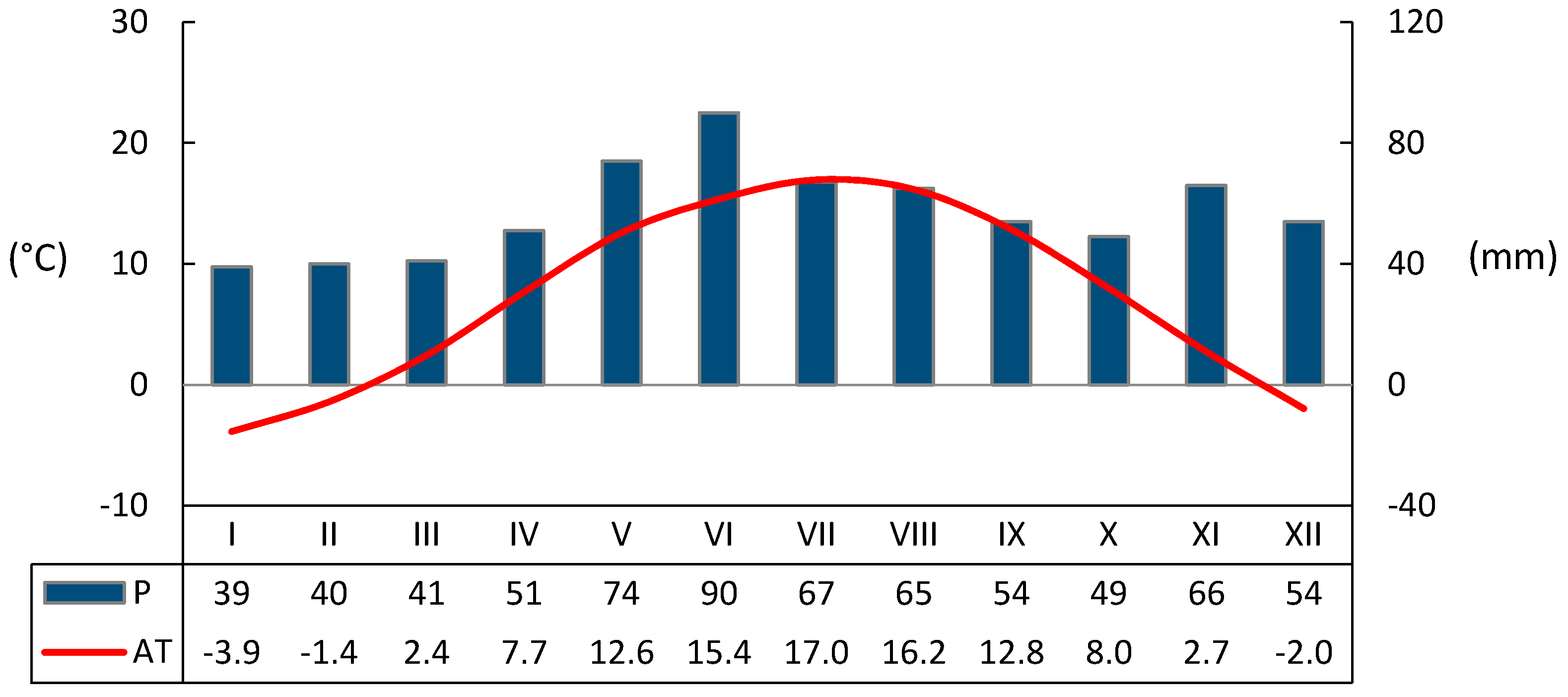
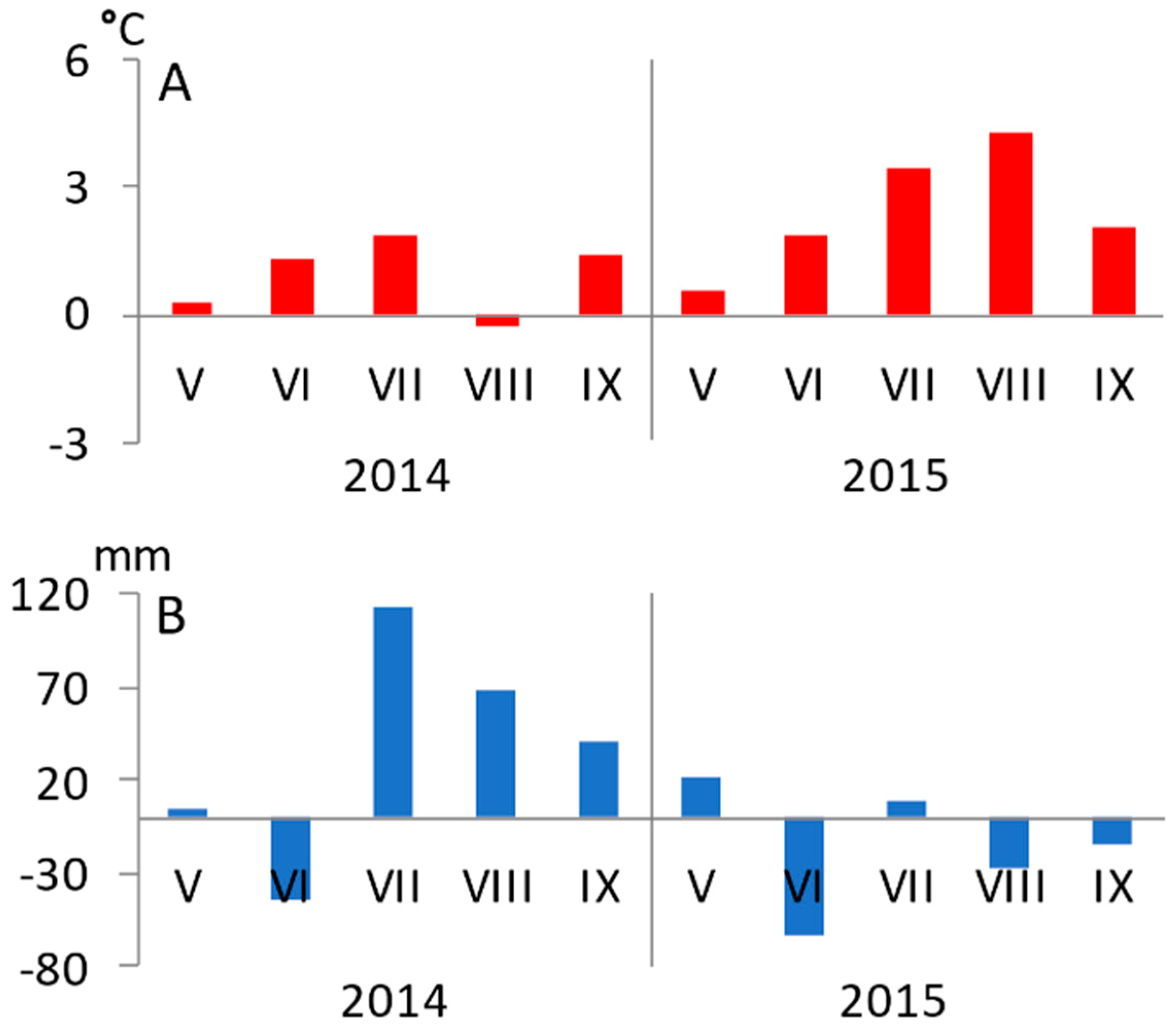
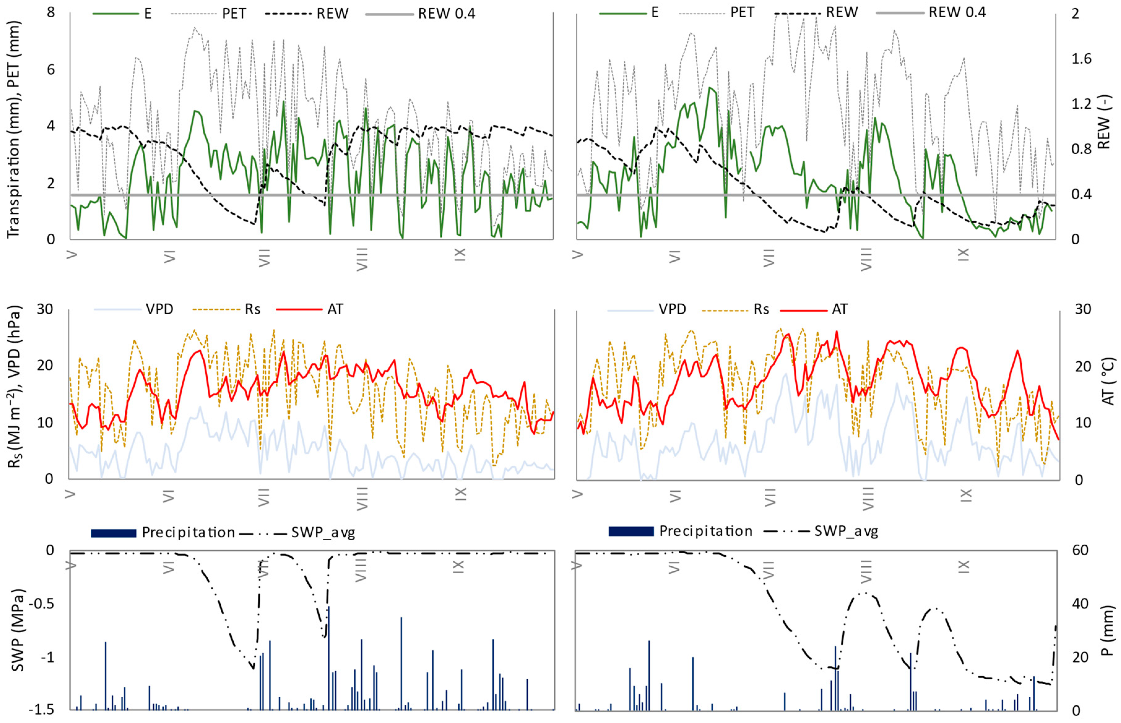
3.1. Seasonal Variation of Environmental Conditions

The growing seasons (May–September) of the years 2014 and 2015 were characterised by mean air temperatures that exceeded the monthly long-term means, except for August 2014, when the mean temperature was slightly (0.2 °C) below normal (Figure 5). The warmest months compared to the normal occurred in 2015, whereas in July, August, and September, the deviations from normal were at a level of +3.5 °C, +4.3 °C, and +2.1 °C. These high temperatures were accompanied by a lack of precipitation, which was documented by the negative deviations from the normal in monthly precipitation totals. The precipitation totals were 62, 26, and 13 mm below normal, in June, August, and September, respectively. Vice versa, in 2014, the monthly precipitation was below the long-term value only in June. The highest positive deviation, 112 mm, from the normal rainfall was detected in July 2014, which reached 168% of normal. The seasonal (May–September) total of precipitation was 534 mm in 2014 and 279 mm in 2015, whereas the precipitation normal for the locality was 350 mm.

Figure 6 shows the seasonal courses of the atmospheric variables as global radiation (R_S), air temperature (AT), vapour pressure deficit (VPD) and potential evapotranspiration (PET). Precipitation distribution within the growing seasons is depicted together with the course of average soil water potential (Figure 6, bottom). Significantly different conditions were observed in two years of interest, which resulted mainly from unequal precipitation occurrences. In comparison with the previous years, the 2015 growing season was characterised by a lack of precipitation (−71 mm compared to normal) and higher values of air temperatures, global radiation and, hence, also of vapour pressure deficit and potential evapotranspiration, particularly during July, August, and September. That resulted in the occurrence of dry episodes, as was evidenced by reduced values of SWP (the hourly values of soil water potential almost reached the value of −1.5 MPa, which is a limit of the equipment) and relative extractable water (REW). In the forest, the soil water deficit (or water stress) was assumed to occur when REW fell below the threshold of 0.4 [66], inducing stomatal regulation in forest trees [56]. However, [69] reported a slightly lower threshold value for a coniferous forest. Based on the REW threshold of 0.4, we detected 20 days in 2014 and 98 days in 2015 with a water deficit. The first day, when the water deficit was found, was DOY 166 (day of the year, 15 June) and DOY 197 (28 June) in 2014 and 2015, respectively. Drought episodes at Bienska dolina plot were rarely interrupted by summer storms, particularly in 2015.

The daily maximum of VPD was 12.8 hPa and 18.8 hPa in 2014 (11 June) and 2015 (7 June), respectively. The values of PET varied in 2014 from 0.5 mm to 7.5 mm per day and in 2015 between 0.6 mm and 8.2 mm per day (with maximal value on 11 and 7 June, respectively). The total amounts of PET per entire season (May–September) were 609 and 716 mm, respectively.

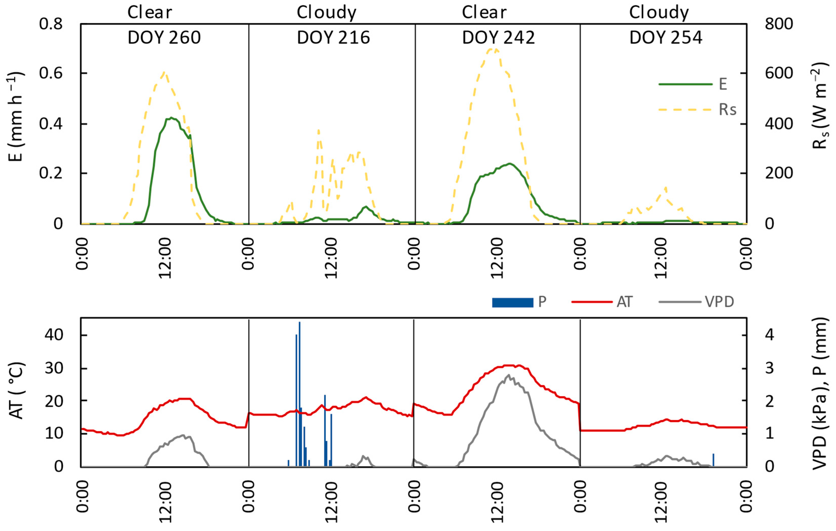
3.2. Seasonal Dynamics of Transpiration

The temporal courses of the daily stand transpiration (E) determined based on sap flow measurements of adult beech trees are shown in Figure 6. Transpiration and the meteorological factors have a synchronised dynamic within the growing season, particularly when soil moisture is not a limiting factor. In conditions with a sufficient water supply, the course of transpiration had almost identical dynamics as the course of PET and also VPD (PET includes the effect of VPD, R_S, and wind speed), which are the expression of atmospheric evaporative demand. Therefore, with the increasing PET, an increase in E was observed. The high evaporative demand related to the high value of global radiation and a corresponding increase in AT, and on the other hand, the decrease in air humidity. However, a temporary reduction in transpiration was detected during rainfall events due to an increase in the water content of the air and the associated changes in atmospheric conditions. Similarly, [70], in their study from Spain, confirmed that beech is strongly affected by water deficit and high temperatures, but these limitations are weakened when cloudiness occurs.

Within the study period, rapid decrease cases in transpiration were observed, particularly in 2015, which were clearly associated with soil water limitations (low values of SWP and REW below 0.4) and were a physiological response of beech stand to water stress. The decrease in E was also associated with high evaporative demand, and the reduction in transpiration was more pronounced as the drought period was prolonged or with the culmination of water deficit. A substantial limitation of beech forest transpiration linked to drought conditions has also been described in many publications [12,19,71,72]. Under drought conditions and/or high atmospheric evaporative demands, plants regulate the transpiration of water by stomatal closure. Stomatal regulation of E is a vital mechanism that allows plants to regulate and optimise CO₂ assimilation versus water loss by evaporation [73]. The total transpiration of the entire measured season in 2014 (May–September) was 359 mm, whereas in 2015, the cumulative values of transpiration reached only 183 mm. Thus, potential seasonal evapotranspiration was 609 and 716 mm in 2014 and 2015, respectively. Hence, the ratio E/PET in 2014 and 2015 was 0.6 and 0.5, respectively. Granier et al. [71] specified beech stand transpiration derived from sap flow measurement as 76 and 72% of total evapotranspiration (eddy covariance technique) for the season from May to October. On average, the transpiration of temperate deciduous forest accounts for 67% of evapotranspiration [2]. In our case, seasonal beech transpiration (from May to September) achieved 59% of PET in 2014, whereas in 2015, it was only 46% (

Table 1. Monthly and seasonal (May–September) sums of transpiration (E) and potential evapotranspiration (PET) in years 2014 and 2015; the ratio E/PET.

	2014			2015
	E (mm)	PET (mm)	E/PET	E (mm)	PET (mm)	E/PET
May	46	119	0.4	58	123	0.5
June	86	165	0.5	106	156	0.7
July	90	149	0.6	72	187	0.4
August	81	104	0.8	73	153	0.5
September	55	72	0.8	19	96	0.2
Season	359	609	0.59	328	716	0.46

). Potential evapotranspiration, according to Penman [65], represents the theoretical value of water, which can be evaporated from the ecosystem provided little or negligible resistance to water flux and no soil water limitation. In times of drought, the plants try to protect against excessive water loss, the stomatal resistance is increasing. The ratio E/PET in Bienska dolina was markable as decreased in July, August, and most in September of 2015. The ratio of transpiration against PET was affected by a deficit of soil water documented by the decreased values of SWP and REW dropped below 0.4. This effect of REW to E/PET ratio was described also by [17] in a sessile oak stand (Quercus petraea).

The highest achieved value of the ratio E/PET was 0.8 and occurred in August and September 2014, the months rich for precipitation and with average evaporation demands. In this month, beech transpiration represented 80% of potential evapotranspiration in the high air evaporative demands and conforming soil moisture conditions. In contrast, the smallest ratio, 0.2, was documented in September 2015, when, due to intensive and prolonged drought duration, the transpiration was only 19 mm compared to the value of potential evapotranspiration of 96 mm.

Within the studied seasons, also observed were relatively higher values of transpiration during the time of reduced values of REW (mostly in 2015). However, significantly reduced E/PET ratio indicated the regulation of transpiration. This phenomenon usually occurred after precipitation events and at the beginning of the period with the decrease in soil water availability. Assuming correctly determined REW values, we can therefore suppose that it was related to the use of water from tree reservoirs in drought conditions, similarly as was described in [12]. In some cases, however, we cannot strictly rule out the usage of water from deeper soil layers or groundwater fractures.

For a detailed display of the diurnal course of transpiration, we chose one sunny/clear day and one day with the occurrence of clouds (rain) in the period with a sufficient supply of soil water (DOY 260 and DOY 216) and also in the period in which there was a deficit of soil water (REW decreased under the value of 0.4, DOY 242 and DOY 254). Figure 7 shows the 20-min variations in transpiration and meteorological factors within days. On clear days, the courses of transpiration and global radiation and vapour pressure deficit were synchronous but lagged in time. The diurnal course of transpiration on clear days had one peak, which occurred after the peak of global radiation. On clear days, the course of transpiration followed the R_S course. With sunrise in the morning and the increase in R_S, transpiration began to increase and peaked around noon: within sufficient soil water conditions at 13:00 and in conditions of water deficit at 14:00. In comparison, the maximum of R_S occurred at 12:00 and 11:20, respectively. Hence, the course of transpiration lagged behind R_S by 60 min when water was not the limiting factor and 160 min in conditions of soil water deficiency. The maximums of AT and VPD were reached at 14:20; thus, the peak occurred 80 min later in day than the peak of transpiration. On the other hand, during drought conditions, it was at 13:40, indicating that the maximal values of AT and VPD occurred 20 min sooner than maximum E. The transpiration rate was significantly limited during soil water deficit compared to days with sufficient soil water supply.

During cloudy days, the typical bell-shaped curve of transpiration was not observed. High air humidity and low VPD values caused significant attenuation of transpiration or it falling to negligible values.

Figure 7. Diurnal dynamics of transpiration (E, 20-min data) and global radiation (R_S), air temperature (AT), vapour pressure deficit (VPD) and precipitation (P) during sunny/clear days and cloudy days in period without soil water deficit (left, DOY 260 and 216) and with soil water deficit (right, DOY 242 and 254). The data are provided in Central European Time (UTC+1).

Figure 7. Diurnal dynamics of transpiration (E, 20-min data) and global radiation (R_S), air temperature (AT), vapour pressure deficit (VPD) and precipitation (P) during sunny/clear days and cloudy days in period without soil water deficit (left, DOY 260 and 216) and with soil water deficit (right, DOY 242 and 254). The data are provided in Central European Time (UTC+1).

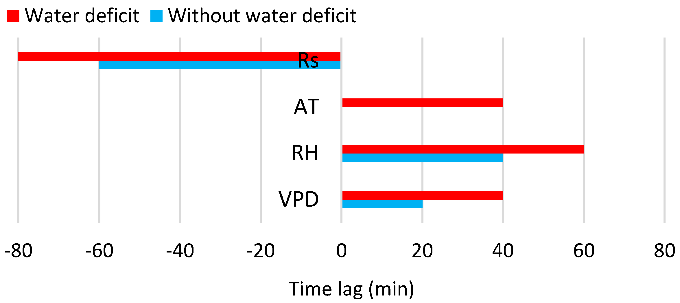
3.3. Relation of Transpiration to Environmental Conditions

Principal component analysis was used to extract a smaller number of common factors, which can represent a large percentage of the variability in the original variables. Therefore, to express the covariances amongst the variables in terms of a small number of meaningful factors. The first three PCA components, only whose eigenvalues were greater than or equal to 1, could together explain 83% of the variance in the data set (

Table 2. Eigenvalues and explained variance by three components on the environmental data (PCA).

Component No.	Eigenvalue	Percent of Variance	Cumulative Percentage
1	3.7	53	53
2	1.1	16	69
3	1.0	14	83

). Up to 53% of the variability could be explained by the first component. The second and third components explained 16% and 14%, respectively. According to

Table 3. Table of component weights (PCA).

Variables	Component 1	Component 2	Component 3
RS	0.45	−0.23	−0.03
AT	0.42	0.09	0.17
RH	−0.46	−0.16	0.00
P	−0.07	−0.19	0.97
VPD	0.48	0.18	0.06
PET	0.42	−0.36	−0.06
SWP	0.05	0.85	0.15

, the first component was positively related mostly to VPD, R_S, PET, AT and negatively to RH. We can conclude, therefore, that the high factor loadings that occurred in the first component represent atmospheric conditions and evaporative demands. The second component explained 16% and was high and positively related to soil water potential and represents the demands for soil water moisture. The third component was positively related to precipitation. Global radiation, vapour pressure deficit, air temperature, and relative humidity were the main atmospheric factors and were included in the subsequent analyses.

A backward stepwise regression was performed to detect the interactive control of stand transpiration by environmental drivers. The input variables were R_S, AT, RH, and VPD. The results of the analysis are shown in

Table 4. Results of fitting a multiple linear regression model to describe the relationship between stand transpiration and global radiation (R_S), air temperature (AT) and relative humidity (RH) as independent variables (variables without time shift: top, variables shifted in time: bottom).

Variable	R2	Model	p < 0.001
RS, AT, RH	0.690	E = 0.0536679 + 0.000295379 RS + 0.00499328 AT − 0.00127058 RH
RS, AT	0.670	E = 0.0834326 + 0.000341555 RS + 0.00679228 AT
RS, RH	0.666	E = 0.171546 + 0.000330795 RS − 0.00181746 RH
AT, RH	0.532	E = 0.163561 + 0.00883183 AT − 0.00279198 RH
Shifted variable	R2	Model	p < 0.001
RS-60, AT+40, RH+20	0.729	E = 0.00707624 + 0.00037642 RS-60 + 0.00342536 AT+40 − 0.000541175 RH+20
RS-60, AT+40	0.726	E = −0.0479013 + 0.000403582 RS-60 + 0.00389637 AT+40
RS-60, RH+20	0.718	E = 0.07679 + 0.000410532 RS-60 − 0.000797576 RH-40
AT+40, RH+20	0.537	E = 0.169809 + 0.00875072 AT+40 − 0.00285242 RH+20

, which provides the regression equations (models) and determination coefficients (R²). All three variables together explained 69% of the variability in stand transpiration (upper part of table). R² significantly decreased when R_S was excluded from the parameters; hence, R_S was the primary driver. The same factors, but shifted in time, explained 73% of the transpiration variability (lower part of the table). The time lags between environmental variables and transpiration were estimated by performing a time-series cross-correlation analysis. In this context, ref [40] described that three variables, namely net radiation, air temperature and vapour pressure deficit together explained 97% of the variations in hourly plant water use in a humid headwater catchment. They also confirmed the major impact of radiation based on the decreased R² of the model when radiation was not considered in regression analysis. The second most important factor was VPD. The study from a water-limited desert ecosystem [43] found that R_S, AT and VPD together explained 84% and 77% of the variance in stand transpiration in 2014 and 2015, respectively. Both studies have consistently stated that water use (sap flux or stand transpiration) was primarily controlled by the availability of energy.

As shown in

Table 5. Regression analysis of stand transpiration and environmental variables shifted in time for 2 categories of soil water conditions: without water deficit versus water deficit.

Variable	Without Water Deficit, REW > 0.4			Water Deficit, REW < 0.4
	Time Lag	R2	Equation	Time Lag	R2	Equation
Rs	−60 min	0.76	y = 0.0035 + 0.0005x *	−80 min	0.69	y = 0.0099 + 0.0004x *
AT	-	0.64	y = 0.0955 − 0.0237x + 0.0014x2 *	+40 min	0.42	y = −0.0408 + 0.0005x + 0.0003x2 *
RH	+40 min	0.54	y = 0.6651 − 0.0094x + 2.8194 × 10−5x2 *	+60 min	0.49	y = 0.5425 − 0.0105x + 5 × 10−5x2 *
VPD	+20 min	0.72	y = −0.0001 + 0.0002x *	+40 min	0.55	y = −0.0207 + 0.1723x − 0.0262x2 *

* p = 0.0000.

and Figure 8, a strong dependence was demonstrated between transpiration and meteorological factors. The correlation between E and VPD in conditions without soil water deficit was linear (R² = 0.72) and in conditions with water deficit, the relationship was best described by a polynomial function (R² = 0.55). The correlation between E and R_S was linear in both cases. In contrast, the correlation between E and AT and RH was polynomial in both cases, but within the relationship between E versus RH, the correlation was negative. The main drivers of transpiration process are mostly considered R_S and VPD (e.g., [17,40,43,74]). The linearity between transpiration and environmental variables was also observed in other studies [40,43,75,76]. For example, [43] observed linear correlation of stand transpiration and R_S, but the relationship between E and VPD was well fitted by a two-degree polynomial function, as well as the relationship between E and AT.

The strongest dependence of transpiration on the environmental variables was primarily found in conditions of sufficient water supply (without water deficit, REW > 0.4). The highest strength of linear correlation was between E and R_S shifted in time by −60 min, where 76% of the variability in transpiration can be explained by changes in global radiation (R² = 0.76). Hence, transpiration was most affected by R_S, which occurred 60 min ‘before’. In the same manner, but in the opposite direction (positive), the tightness of the relationship between transpiration and VPD was higher when VPD was shifted in time by +20 min (R² = 0.72) (the VPD 20 min ‘after’ transpiration). Similarly, the tightest relationship between E and RH was confirmed by RH shifted in time of +40 min. The time lag was not confirmed within air temperature, although it is possible that the time shift was less than 20 min. Global radiation is the main driver that determines other variables, and their course tends to lag behind. That may be the reason why only time lag of R_S is negative.

The effect of drought stress was also reflected by a notable decrease in the dependence of transpiration from the tested variables. R² decreased to 0.69 (from 0.76), 0.42 (from 0.64), 0.49 (from 0.54) and to 0.55 (from 0.72) for E versus R_S, AT, RH and VPD, respectively (Table 5). These observations are consistent with the conclusions of [74]. Besides that, based on linear or polynomial regression, as a consequence of drought stress, the time shifts were prolonged by an average of 25 min (Figure 9). Hence, the course of transpiration lagged behind the course of global radiation by 60 min and by 80 min in conditions without water deficit and with water deficit, respectively. This phenomenon may be related to the plant’s water-saving strategy. At the same time, water from the trunk’s reserves is used more during the soil water deficit [12].

Several authors have observed the time shift in the daily course of transpiration compared to the course of various environmental factors. Xu and Yu [43] studied hysteresis loops in shrub species and described the time legs in 2014 between transpiration and R_S, AT and VPD at an average of 1.5, 4.5, and 4.5 h, respectively. This study from desert ecosystem pointed that in 2015 maximum transpiration occurred after maximum R_S for 1.5 h, but before AT and VPD (for 2 h), which approximately corresponded with our results. The authors found seasonal patterns and as a possible cause marked stem water storage. Carrasco et al. [77] and Xu and Yu [43] also reported the water storage in the tree trunk having a role in time shift. Similarly, [40] analysed the relationships between transpiration of Scots pine and meteorological variables and also observed time lags and their seasonality. They found that sap flow lagged behind daily changes in meteorological variables indicated by phase shifts. Some studies claimed that the time shifts could be connected to the water conservation or self-protection mechanism of plants through stomatal control. Therefore, when the transpiration/sap flow reached the maxima earlier than environmental drivers (mainly VPD), further increases in the latter did not lead to more water loss by transpiration due to stomatal closure in response to meteorological changes [75,76]. In our study, the results pointed to the occurrence of the transpiration maxima before the peak of VPD, AT and RH. On the other hand, the situation was different for the courses of R_S. At the same time, the impact of the soil water deficit to the time lags was confirmed. O’Grady et al. [42] also described larger lags in dry than in wet seasons in Australian savannas (eucalyptus). A similar effect was identified by [78].

The relationship between E and VPD in the conditions of sufficient soil moisture was best described by a linear equation (coincided with [43]), and in the period of drought stress, this relationship changed and was described by a polynomial function. During water non-limited conditions, the stand transpiration increased linearly with the increase in VPD, because stomatal control of transpiration was minimal, and in drought conditions, the transpiration increased rapidly only until an unspecified threshold in VPD was gained. Then, transpiration was already inhibited. This finding may indicate that high values of VPD drive the stomatal regulation of transpiration. Similarly, [71] stated that in conditions of well-watered soil, beech shows a strong link between transpiration and VPD, but in conditions with limited soil water, canopy conductance decreases and is weakly related to atmospheric water demands. MacKay et al. [16] marked VPD as the main control of water loss in the forest, whereas soil moisture had an effect when the content of soil water decreased below a site-specific threshold during the growing season. Many authors have described the threshold control of VPD on transpiration, although the threshold value tends to be slightly different (1.2–2 kPa) [43,77,79,80]. However, [81] reported that hourly sap flow in northern hardwood forest declined in dry soil when VPD exceeded 1 kPa.

Transpiration is driven by energy income and connected evaporative demand, provided enough extractable soil water. Global radiation is the main driver that determines the course of other variables, and their course tends to lag behind. When assessing the causes of the delayed course of transpiration, it is also necessary to take into account that sap flow measurements take place on the tree trunk, whereas evaporation occurs in the tree canopy (the evaporating surface involves leaves). As was confirmed, there exist time shifts in sap flow measured in different parts of the tree (stem base versus crown part) caused by the use of water stored in the trunk for transpiration. The stored water is depleted in the morning and refilled during the night (nocturnal sap flow), depending on the weather. The amount of stored water depends on the species and dimensions of trees and varies in time. Čermák et al. [82] stated that on a daily basis (but not for the entire +growing season), the volume of water withdrawn from storage was equivalent to the water refilled to storage. The storage water on clear days was ca. 23% of the daily sap flow in old-growth Douglas-fir tree. For comparison, [83] for Douglas-fir stated water stored in xylem was 20 to 25% of total daily water use in 60-m trees, whereas in 15-m trees it was only 7%. For Oregon white oak stored water accounted for 10–23% of total daily water use in 25-m tall trees, whereas stored water comprised 9–3% in 10-m trees. The research of [77] indicated that tree trunk water storage contributes from 6 to 28% of the daily water budget of large trees depending on the species and [44] found the strong relationship between stored water use and DBH, sapwood area and leaf area. Wang et al. [40] determined nocturnal sap flow as 17% of the total sap flow on average in Scots pine in a humid low-energy headwater catchment and stated that trunk water storage would contribute to hysteresis and time lags between sap flow and meteorological forcing.

We can conclude that both the water storage and its use for morning transpiration and also atmospheric drivers can cause time lags. However, it is important to recognise their existence to incorporate them into water flux modelling and when investigating plant responses to changing environmental drivers.

4. Conclusions

This paper has evaluated the seasonal and diurnal dynamics of transpiration as a component of potential evapotranspiration and examined the environmental drivers’ control of beech transpiration and the impact of water deficit on this relation. The experiment was based on the in-situ measurement of sap flow and accompanying measurement of environmental variables and soil water potential. It was found that seasonal beech transpiration (from May to September) achieved 59% of potential evapotranspiration in 2014, whereas in 2015, it was only 46%. During the studied growing seasons 2014 and 2015, soil water deficit led to the radical limitation of transpiration and affected the relationship between transpiration and environmental drivers. The ratio of transpiration (E) against potential evapotranspiration (PET) was significantly affected by the deficit of soil water and in dry September 2015 decreased to the value of 0.2. The maximum monthly value (0.8) of E/PET was recorded in August and September 2014. These months were characterised by above-normal precipitation totals, REW values above 0.4 and SWP values close to 0 MPa.

A time lag was demonstrated between the course of transpiration and environmental factors on a diurnal basis. Performing a time series cross-correlation, time lags for environmental variables were observed. An application of the time lags within the analysis increased the strength of the association between transpiration and the variables. We determined that the variation in beech transpiration was tightly associated with alterations in global radiation (R_S), air temperature (AT) and air humidity (RH). A multiple regression model constructed from these three environmental variables explained 69% of the variability in the beech stand transpiration. When we used time-shifted variables in the model (based on the cross-correlation), the model explained 73% of the transpiration variability.

References

1. Jasechko, S.; Sharp, Z.D.; Gibson, J.J.; Birks, S.J.; Yi, Y.; Fawcett, P.J. Terrestrial water fluxes dominated by transpiration. Nature 2013, 496, 347–350. [Google Scholar] [CrossRef] [PubMed]
2. Schlesinger, W.H.; Jasechko, S. Transpiration in the global water cycle. Agric. For. Meteorol. 2014, 189–190, 115–117. [Google Scholar] [CrossRef]
3. Kučera, J.; Brito, P.; Jiménez, M.S.; Urban, J. Direct Penman–Monteith parameterization for estimating stomatal conductance and modeling sap flow. Trees 2016. [Google Scholar] [CrossRef] [Green Version]
4. Lu, J.; Sun, G.; McNulty, S.G.; Amatya, D.M. Modeling actual evapotranspiration from forested watersheds across the southeastern United States. J. Am. Water Resour. Assoc. 2003, 39, 886–896. [Google Scholar] [CrossRef]
5. Zheng, H.; Yu, G.; Wang, Q.; Zhu, X.; He, H.; Wang, Y.; Zhang, J.; Li, Y.; Zhao, L.; Zhao, F.; et al. Spatial variation in annual actual evapotranspiration of terrestrial ecosystems in China: Results from eddy covariance measurements. J. Geogr. Sci. 2016, 26, 1391–1411. [Google Scholar] [CrossRef]
6. Ferreira, M.I. Stress coefficients for soil water balance combined with water stress indicators for irrigation scheduling of woody crops. Horticulturae 2017, 3, 38. [Google Scholar] [CrossRef] [Green Version]
7. Ferreira, M.I.; Paço, T.A.; Silvestre, J.; Silva, R.M. Evapotranspiration estimates and water stress indicators for irrigation scheduling in woody plants. In Agricultural Water Management Research Trends; Nova Science Publishers, Inc.: New York, NY, USA, 2008; pp. 129–170. [Google Scholar]
8. Čermák, J.; Kučera, J.; Nadezhdina, N. Sap flow measurements with some thermodynamic methods, flow integration within trees and scaling up from sample trees to entire forest stands. Trees 2004, 18, 529–546. [Google Scholar] [CrossRef]
9. Köstner, B.; Falge, E.; Alsheimer, M. Sap Flow Measurements. Struct. Role Submerg. Macrophytes Lakes 2017, 99–112. [Google Scholar] [CrossRef]
10. Tatarinov, F.A.; Kučera, J.; Cienciala, E. The analysis of physical background of tree sap flow measurement based on thermal methods. Meas. Sci. Technol. 2005, 16, 1157–1169. [Google Scholar] [CrossRef]
11. Kaufmann, M.R.; Kelliher, F.M. Measuring transpiration rates. In Techniques and Approaches in Forest Tree Ecophysiology; Lassoie, J.P., Hinckley, T.M., Eds.; CRC Press: Boca Raton, FL, USA, 1991; pp. 117–140. [Google Scholar]
12. Betsch, P.; Bonal, D.; Breda, N.; Montpied, P.; Peiffer, M.; Tuzet, A.; Granier, A. Drought effects on water relations in beech: The contribution of exchangeable water reservoirs. Agric. For. Meteorol. 2011, 151, 531–543. [Google Scholar] [CrossRef]
13. De Swaef, T.; De Schepper, V.; Vandegehuchte, M.W.; Steppe, K. Stem diameter variations as a versatile research tool in ecophysiology. Tree Physiol. 2015, 35, 1047–1061. [Google Scholar] [CrossRef] [PubMed]
14. Tenhunen, J.D.; Valentini, R.; Köstner, B.; Zimmermann, R.; Granier, A. Variation in forest gas exchange at landscape to continental scales. Ann. For. Sci. 1998, 55, 1–11. [Google Scholar] [CrossRef] [Green Version]
15. Davi, H.; Dufrêne, E.; Granier, A.; Le Dantec, V.; Barbaroux, C.; François, C.; Bréda, N. Modelling carbon and water cycles in a beech forest. Part II: Validation of the main processes from organ to stand scale. Ecol. Modell. 2005, 185, 387–405. [Google Scholar] [CrossRef] [Green Version]
16. MacKay, S.L.; Arain, M.A.; Khomik, M.; Brodeur, J.J.; Schumacher, J.; Hartmann, H.; Peichl, M. The impact of induced drought on transpiration and growth in a temperate pine plantation forest. Hydrol. Process. 2012, 26, 1779–1791. [Google Scholar] [CrossRef] [Green Version]
17. Breda, N.; Granier, A. Intra and interannual variations of transpiration, leaf area index and radial growth of sessile oak stand (Quercus petraea). Ann. Sci. For. 1996, 53, 521–536. [Google Scholar] [CrossRef] [Green Version]
18. Eamus, D.; Boulain, N.; Cleverly, J.; Breshears, D.D. Global change-type drought-induced tree mortality: Vapor pressure deficit is more important than temperature per se in causing decline in tree health. Ecol. Evol. 2013, 3, 2711–2729. [Google Scholar] [CrossRef] [PubMed]
19. Kirchen, G.; Calvaruso, C.; Granier, A.; Redon, P.O.; Van der Heijden, G.; Bréda, N.; Turpault, M.P. Local soil type variability controls the water budget and stand productivity in a beech forest. For. Ecol. Manag. 2017, 390, 89–103. [Google Scholar] [CrossRef]
20. Jiao, L.; Lu, N.; Fang, W.; Li, Z.; Wang, J.; Jin, Z. Determining the independent impact of soil water on forest transpiration: A case study of a black locust plantation in the Loess Plateau, China. J. Hydrol. 2019, 572, 671–681. [Google Scholar] [CrossRef]
21. Lüttschwager, D.; Jochheim, H. Drought primarily reduces canopy transpiration of exposed beech trees and decreases the share of water uptake from deeper soil layers. Forests 2020, 11, 537. [Google Scholar] [CrossRef]
22. Schwinning, S. The ecohydrology of roots in rocks. Ecohydrology 2010, 3, 238–245. [Google Scholar] [CrossRef]
23. Eliades, M.; Bruggeman, A.; Lubczynski, M.W.; Christou, A.; Camera, C.; Djuma, H. The water balance components of Mediterranean pine trees on a steep mountain slope during two hydrologically contrasting years. J. Hydrol. 2018, 562, 712–724. [Google Scholar] [CrossRef]
24. IPCC 2018. Global warming of 1.5 °C. An IPCC Special Report on the impacts of global warming of 1.5 °C above pre-industrial levels and related global greenhouse gas emission pathways, in the context of strengthening the global response to the threat of climate change. In Summary for Policymakers; Masson-Delmotte, V., Zhai, P., Pörtner, H.O., Roberts, D., Skea, J., Shukla, P.R., Pirani, A., Moufouma-Okia, W., Péan, C., Pidcock, R., et al., Eds.; World Meteorological Organization: Geneva, Switzerland, 2019; p. 32. [Google Scholar]
25. Rowell, D.P.; Jones, R.G. Causes and uncertainty of future summer drying over Europe. Clim. Dyn. 2006, 27, 281–299. [Google Scholar] [CrossRef]
26. IPCC 2014. Climate Change 2014: Impacts, Adaptation, and Vulnerability. Part. B: Regional Aspects. Europe. Contribution of Working Group II to the Fifth Assessment Report of the Intergovernmental Panel on Climate Change; Cambridge University Press: Cambridge, UK, 2014. [Google Scholar]
27. Centritto, M.; Tognetti, R.; Leitgeb, E.; Střelcová, K.; Cohen, S. Chapter 3 Above Ground Processes: Anticipating Climate Change Influences. In Forest Management and the Water Cycle: An Ecosystem-Based Approach; Bredemeier, M., Cohen, S., Godbold, D.L., Lode, E., Pichler, V., Schleppi, P., Eds.; Springer: Dordrecht, The Netherlands, 2011; Volume 212, pp. 263–289. ISBN 978-90-481-9833-7. [Google Scholar]
28. Williams, A.P.; Allen, C.D.; Macalady, A.K.; Griffin, D.; Woodhouse, C.A.; Meko, D.M.; Swetnam, T.W.; Rauscher, S.A.; Seager, R.; Grissino-Mayer, H.D.; et al. Temperature as a potent driver of regional forest drought stress and tree mortality. Nat. Clim. Chang. 2013, 3, 292–297. [Google Scholar] [CrossRef]
29. Bertini, G.; Amoriello, T.; Fabbio, G.; Piovosi, M. Forest growth and climate change: Evidences from the ICP-Forests intensive monitoring in Italy. IForest 2011, 4, 262–267. [Google Scholar] [CrossRef] [Green Version]
30. Chen, K.; Dorado-Linan, I.; Akhmetzyanov, L.; Gea-Izquierdo, G.; Zlatanov, T.; Menzell, A. Influence of climate drivers and the North Atlantic Oscillation on beech growth at marginal sites across the Mediterranean. Clim. Res. 2015, 66, 229–242. [Google Scholar] [CrossRef]
31. Bréda, N.; Huc, R.; Granier, A.; Dreyer, E. Temperate forest tree and stands under severe drought: A review of ecophysiological responses, adaptation processes and long-term consequences. Ann. Sci. For. 2006, 63, 625–644. [Google Scholar] [CrossRef] [Green Version]
32. McDowell, N.G.; Beerling, D.J.; Breshears, D.D.; Fisher, R.A.; Raffa, K.F.; Stitt, M. The interdependence of mechanisms underlying climate-driven vegetation mortality. Trends Ecol. Evol. 2011, 26, 523–532. [Google Scholar] [CrossRef]
33. Cailleret, M.; Jansen, S.; Robert, E.M.R.; Desoto, L.; Aakala, T.; Antos, J.A.; Beikircher, B.; Bigler, C.; Bugmann, H.; Caccianiga, M.; et al. A synthesis of radial growth patterns preceding tree mortality. Glob. Chang. Biol. 2017, 23, 1675–1690. [Google Scholar] [CrossRef]
34. Allen, R.G.; Pereira, L.S.; Raes, D.; Smith, M. Crop. Evapotranspiration—Guidelines for Computing Crop Water Requirements—FAO Irrigation and Drainage Paper 56; Food and Agriculture Organization of the United Nations: Rome, Italy, 1998. [Google Scholar]
35. Buckley, T.N.; Mott, K.A.; Farquhar, G.D. A hydromechanical and biochemical model of stomatal conductance. Plant Cell Environ. 2003, 26, 1767–1785. [Google Scholar] [CrossRef] [Green Version]
36. Buckley, T.N.; Turnbull, T.L.; Adams, M.A. Simple models for stomatal conductance derived from a process model: Cross-validation against sap flux data. Plant Cell Environ. 2012, 35, 1647–1662. [Google Scholar] [CrossRef]
37. Whitley, R.; Taylor, D.; Macinnis-Ng, C.; Zeppel, M.; Yunusa, I.; O’Grady, A.; Froend, R.; Medlyn, B.; Eamus, D. Developing an empirical model of canopy water flux describing the common response of transpiration to solar radiation and VPD across five contrasting woodlands and forests. Hydrol. Process. 2013, 27, 1133–1146. [Google Scholar] [CrossRef]
38. Wang, H.; Guan, H.; Simmons, C.T. Modeling the environmental controls on tree water use at different temporal scales. Agric. For. Meteorol. 2016, 225, 24–35. [Google Scholar] [CrossRef] [Green Version]
39. Hong, L.; Guo, J.; Liu, Z.; Wang, Y.; Ma, J.; Wang, X.; Zhang, Z. Time-lag effect between sap flow and environmental factors of Larix principis-rupprechtii Mayr. Forests 2019, 10, 971. [Google Scholar] [CrossRef] [Green Version]
40. Wang, H.; Tetzlaff, D.; Soulsby, C. Hysteretic response of sap flow in Scots pine (Pinus sylvestris) to meteorological forcing in a humid low-energy headwater catchment. Ecohydrology 2019, 12. [Google Scholar] [CrossRef]
41. Zhang, R.; Xu, X.; Liu, M.; Zhang, Y.; Xu, C.; Yi, R.; Luo, W.; Soulsby, C. Hysteresis in sap flow and its controlling mechanisms for a deciduous broad-leaved tree species in a humid karst region. Sci. China Earth Sci. 2019, 62, 1744–1755. [Google Scholar] [CrossRef]
42. O’Grady, A.P.; Worledge, D.; Battaglia, M. Constraints on transpiration of Eucalyptus globulus in southern Tasmania, Australia. Agric. For. Meteorol. 2008, 148, 453–465. [Google Scholar] [CrossRef]
43. Xu, S.; Yu, Z. Environmental control on transpiration: A case study of a desert ecosystem in northwest china. Water 2020, 12, 1211. [Google Scholar] [CrossRef]
44. Verbeeck, H.; Steppe, K.; Nadezhdina, N.; Op De Beeck, M.; Deckmyn, G.; Meiresonne, L.; Lemeur, R.; Čermák, J.; Ceulemans, R.; Janssens, I.A. Stored water use and transpiration in Scots pine: A modeling analysis with ANAFORE. Tree Physiol. 2007, 27, 1671–1685. [Google Scholar] [CrossRef] [Green Version]
45. Chen, L.; Zhang, Z.; Li, Z.; Tang, J.; Caldwell, P.; Zhang, W. Biophysical control of whole tree transpiration under an urban environment in Northern China. J. Hydrol. 2011, 402, 388–400. [Google Scholar] [CrossRef]
46. Zeppel, M.J.B.; Murray, B.R.; Barton, C.; Eamus, D. Seasonal responses of xylem sap velocity to VPD and solar radiation during drought in a stand of native trees in temperate Australia. Funct. Plant Biol. 2004, 31, 461–470. [Google Scholar] [CrossRef]
47. Geßler, A.; Keitel, C.; Kreuzwieser, J.; Matyssek, R.; Seiler, W.; Rennenberg, H. Potential risks for European beech (Fagus sylvatica L.) in a changing climate. Trees Struct. Funct. 2007, 21, 1–11. [Google Scholar] [CrossRef]
48. Fritz, P. (Ed.) Ökologischer Waldumbau in Deutschland (Ecological Reconstruction of Forests in Germany); Oekom Verlag: Munich, Germany, 2006; ISBN 978-3-86581-001-4. [Google Scholar]
49. Dedrick, S.; Spiecker, H.; Orazio, C.; Tomé, M.; Martinez, I. Plantation or Conversion—The Debate! Ideas Presented and Discussed at a Joint EFI Project-Centre Conference Held 21–23 May 2006 in Freiburg, Germany; European Forest Institute: Joensuu, Finland, 2007; ISBN 9789525453164. [Google Scholar]
50. Green Report: Report on Forestry in the Slovak Republic per Year 2018; Ministry of Agriculture and Rural Development of the Slovak Republic and National Forest Centre: Bratislava, Slovakia, 2019.
51. Jung, T. Beech decline in Central Europe driven by the interaction between Phytophthora infections and climatic extremes. For. Pathol. 2009, 39, 73–94. [Google Scholar] [CrossRef]
52. Mátyás, C.; Berki, I.; Czúcz, B.; Gálos, B.; Móricz, N.; Rasztovits, E. Future of beech in Southeast Europe from the perspective of evolutionary ecology. Acta Silv. Lignaria Hung. 2010, 6, 91–110. [Google Scholar]
53. Corcobado, T.; Cech, T.L.; Brandstetter, M.; Daxer, A.; Hüttler, C. Decline of European Beech in Austria: Involvement of Phytophthora spp. and Contributing Biotic and Abiotic Factors. Forests 2020, 11, 859. [Google Scholar] [CrossRef]
54. Střelcová, K.; Matejka, F.; Kučera, J. Beech stand transpiration assessment—Two methodical approaches. Ekologia 2004, 22, 147–162. [Google Scholar]
55. Thiel, D.; Kreyling, J.; Backhaus, S.; Beierkuhnlein, C.; Buhk, C.; Egen, K.; Huber, G.; Konnert, M.; Nagy, L.; Jentsch, A. Different reactions of central and marginal provenances of fagus sylvatica to experimental drought. Eur. J. For. Res. 2014, 133, 247–260. [Google Scholar] [CrossRef]
56. Granier, A.; Reichstein, M.; Bréda, N.; Janssens, I.A.; Falge, E.; Ciais, P.; Grunwald, T.; Aubinet, M.; Berbigier, P.; Bernhofer, C.; et al. Evidence for soil water control on carbon and water dynamics in European forests during the extremely dry year: 2003. Agric. For. Meteorol. 2007, 143, 123–145. [Google Scholar] [CrossRef]
57. van der Maaten-Theunissen, M.; Bümmerstede, H.; Iwanowski, J.; Scharnweber, T.; Wilmking, M.; van der Maaten, E. Drought sensitivity of beech on a shallow chalk soil in northeastern Germany—A comparative study. For. Ecosyst. 2016, 3, 24. [Google Scholar] [CrossRef] [Green Version]
58. Zimmermann, J.; Hauck, M.; Dulamsuren, C.; Leuschner, C. Climate Warming-Related Growth Decline Affects Fagus sylvatica, But Not Other Broad-Leaved Tree Species in Central European Mixed Forests. Ecosystems 2015, 18, 560–572. [Google Scholar] [CrossRef]
59. Decuyper, M.; Chávez, R.O.; Čufar, K.; Estay, S.A.; Clevers, J.G.P.W.; Prislan, P.; Gričar, J.; Črepinšek, Z.; Merela, M.; de Luis, M.; et al. Spatio-temporal assessment of beech growth in relation to climate extremes in Slovenia—An integrated approach using remote sensing and tree-ring data. Agric. For. Meteorol. 2020, 287, 107925. [Google Scholar] [CrossRef]
60. Scharnweber, T.; Manthey, M.; Criegee, C.; Bauwe, A.; Schröder, C.; Wilmking, M. Drought matters—Declining precipitation influences growth of Fagus sylvatica L. and Quercus robur L. in north-eastern Germany. For. Ecol. Manag. 2011, 262, 947–961. [Google Scholar] [CrossRef]
61. Gennaretti, F.; Ogée, J.; Sainte-Marie, J.; Cuntz, M. Mining ecophysiological responses of European beech ecosystems to drought. Agric. For. Meteorol. 2020, 280. [Google Scholar] [CrossRef]
62. Zlatník, A. Overview of groups of geobiocoene types originally wooded or shrubed. Zprávy Geogr. ČSAV Brně 1976, 13, 55–56. (In Czech) [Google Scholar]
63. FAO. World Reference Base for Soil Resources 2014. International Soil Classification System for Naming Soils and Creating Legends for Soil Maps. World Soil Resources Reports No. 106. Update 2015; FAO: Rome, Italy, 2015; ISBN 9789251083697. [Google Scholar]
64. Lapin, M.; Faško, P.; Melo, M.; Šťastný, P.; Tomlain, J. Klimatické oblasti [Climatic Regions]. In Atlas Krajiny Slovenskej Republiky [Landscape Atlas of the Slovak Republic]; Miklos, L., Ed.; Ministry of Environment of the Slovak Republic: Bratislava, Czechoslovakia, 2002; p. 334. [Google Scholar]
65. Penman, H.L. Natural evaporation from open water, bare soil, and grass. Proc. R. Soc. 1948, A193, 120–146. [Google Scholar]
66. Granier, A.; Bréda, N.; Biron, P.; Villette, S. A lumped water balance model to evaluate duration and intensity of drought constraints in forest stands. Ecol. Modell. 1999, 116, 269–283. [Google Scholar] [CrossRef]
67. Kučera, J.; Čermák, J.; Penka, M. Improved thermal method of continual recording the transpiration flow rate dynamics. Biol. Plant 1977, 19, 413–420. [Google Scholar]
68. Jiří Kučera—Environmental Measuring Systems Sap Flow System EMS 81. User’s Manual. 2nd Issue. Available online: http://www.emsbrno.cz/r.axd/pdf_v_EMS81__usermanual_u_pdf.jpg?ver= (accessed on 29 November 2020).
69. Lagergren, F.; Lindroth, A. Transpiration response to soil moisture in pine and spruce trees in Sweden. Agric. For. Meteorol. 2002, 112, 67–85. [Google Scholar] [CrossRef]
70. Rozas, V.; Camarero, J.J.; Sangüesa-Barreda, G.; Souto, M.; García-González, I. Summer drought and ENSO-related cloudiness distinctly drive Fagus sylvatica growth near the species rear-edge in northern Spain. Agric. For. Meteorol. 2015, 201, 153–164. [Google Scholar] [CrossRef] [Green Version]
71. Granier, A.; Biron, P.; Lemoine, D. Water balance, transpiration and canopy conductance in two beech stands. Agric. For. Meteorol. 2000, 100, 291–308. [Google Scholar] [CrossRef]
72. Gebauer, T.; Horna, V.; Leuschner, C. Canopy transpiration of pure and mixed forest stands with variable abundance of European beech. J. Hydrol. 2012, 442–443, 2–14. [Google Scholar] [CrossRef]
73. Haworth, M.; Killi, D.; Materassi, A.; Raschi, A.; Centritto, M. Impaired stomatal control is associated with reduced photosynthetic physiology in crop species grown at elevated [CO2]. Front. Plant. Sci. 2016, 7, 1–13. [Google Scholar] [CrossRef] [PubMed] [Green Version]
74. Matejka, F.; Střelcová, K.; Hurtalová, T.; Gömöryová, E.; Ditmarová, Ľ. Seasonal changes in transpiration and soil water content in a spruce primeval forest during a dry period. In Bioclimatology and Natural Hazards; Střelcová, K., Mátyás, C., Kleidon, A., Lapin, M., Matejka, F., Blaženec, M., Škvarenina, J., Holécy, J., Eds.; Springer: Dordrecht, Germany, 2009; pp. 197–206. [Google Scholar]
75. Tie, Q.; Hu, H.; Tian, F.; Guan, H.; Lin, H. Environmental and physiological controls on sap flow in a subhumid mountainous catchment in North China. Agric. For. Meteorol. 2017, 240–241, 46–57. [Google Scholar] [CrossRef]
76. Bai, Y.; Zhu, G.; Su, Y.; Zhang, K.; Han, T.; Ma, J.; Wang, W.; Ma, T.; Feng, L. Hysteresis loops between canopy conductance of grapevines and meteorological variables in an oasis ecosystem. Agric. For. Meteorol. 2015, 214–215, 319–327. [Google Scholar] [CrossRef]
77. Carrasco, L.O.; Bucci, S.J.; Di Francescantonio, D.; Lezcano, O.A.; Campanello, P.I.; Scholz, F.G.; Rodríguez, S.; Madanes, N.; Cristiano, P.M.; Hao, G.Y.; et al. Water storage dynamics in the main stem of subtropical tree species differing in wood density, growth rate and life history traits. Tree Physiol. 2015, 35, 354–365. [Google Scholar] [CrossRef] [PubMed] [Green Version]
78. Tuzet, A.; Perrier, A.; Leuning, R. A coupled model of stomatal conductance and photosynthesis for winter wheat. Plant Cell Environ. 2003, 26, 1097–1116. [Google Scholar] [CrossRef]
79. Poyatos, R.; Llorens, P.; Piñol, J.; Rubio, C. Response of Scots pine (Pinus sylvestris L.) and pubescent oak (Quercus pubescens Willd.) to soil and atmospheric water deficits under Mediterranean mountain climate. Ann. For. Sci. 2008, 65, 306. [Google Scholar] [CrossRef]
80. Priwitzer, T.; Kurjak, D.; Kmeť, J.; Sitková, Z.; Leštianska, A. Photosynthetic response of European beech to atmospheric and soil drought. For. J. 2014, 60, 31–37. [Google Scholar] [CrossRef] [Green Version]
81. Bovard, B.D.; Curtis, P.S.; Vogel, C.S.; Su, H.B.; Schmid, H.P. Environmental controls on sap flow in a northern hardwood forest. Tree Physiol. 2005, 25, 31–38. [Google Scholar] [CrossRef] [Green Version]
82. Čermák, J.; Kučera, J.; Bauerle, W.L.; Phillips, N.; Hinckley, T.M. Tree water storage and its diurnal dynamics related to sap flow and changes in stem volume in old-growth Douglas-fir trees. Tree Physiol. 2007, 27, 181–198. [Google Scholar] [CrossRef]
83. Phillips, N.G.; Ryan, M.G.; Bond, B.J.; McDowell, N.G.; Hinckley, T.M.; Čermák, J. Reliance on stored water increases with tree size in three species in the Pacific Northwest. Tree Physiol. 2003, 23, 237–245. [Google Scholar] [CrossRef] [Green Version]
Figure 1. Location of the experimental plot Bienska dolina in central Slovakia (SK), Central Europe (left) and design of the experimental plot showing crown projections of all beech trees, position of selected sample trees and soil probes (right).
Water 12 03437 g001
Figure 2. Number of trees in DBH and height classes (interval of the class is 3 cm and 3 m, respectively) within the experimental plot area (608 m2).
Water 12 03437 g002
Figure 3. Monthly averages (normals) of mean air temperature (AT, °C) and precipitation totals (P, mm) for the Bienska dolina area, calculated based on reference period 1961–1990 data (January–December; in Roman numerals I–XII).
Water 12 03437 g003
Figure 5. Deviations in monthly (May–September; in Roman numerals V–IX) air temperature (part A; °C) and precipitation totals (part B; mm) from long-term mean (normal) of 1961–1990.
Water 12 03437 g005
Figure 6. Seasonal dynamics of transpiration and potential evapotranspiration (PET) during vegetation season of 2014 (left) and 2015 (right) and the course of relative extractable water (REW) with a marked threshold of 0.4 (top); daily values of global radiation (RS) vapour pressure deficit (VPD) and average air temperature (AT) (middle); daily values of average soil water potential and precipitation totals (P) (bottom).
Water 12 03437 g006
Figure 8. Relationships between 20-min values of transpiration (E) computed from sap flow measurements (in 2014, 2015) and environmental drivers: global radiation (RS), air temperature (AT) vapour pressure deficit (VPD) and relative humidity (RH) shifted in time (+ or − min); data divided into two categories according to the state of REW: left/blue when REW > 0.4 (without water deficit) and right/red when REW < 0.4 (with water deficit).
Water 12 03437 g008
Figure 9. Changes in time lags for conditions with water deficit (REW < 0.4) and without water deficit (REW > 0.4).
Water 12 03437 g009