Coupling Sediment Transport Dynamics with Sediment and Discharge Sources in a Glacial Andean Basin


1
Department of Ecosystems and Environments, Pontificia Universidad Católica de Chile, Macul, Santiago 7810000, Chile
2
Institute of Geography, Pontificia Universidad Católica de Chile, Macul, Santiago 7810000, Chile
3
School of Geography, University of Lincoln, Lincoln LN6 7TS, UK
*
Author to whom correspondence should be addressed.
Water 2020, 12(12), 3452; https://doi.org/10.3390/w12123452
Submission received: 28 October 2020
/
Revised: 29 November 2020
/
Accepted: 7 December 2020
/
Published: 9 December 2020
(This article belongs to the Special Issue Fluvial Processes and Denudation)
Abstract
:Suspended and bedload transport dynamics on rivers draining glacierized basins depend on complex processes of runoff generation together with the degree of sediment connectivity and coupling at the basin scale. This paper presents a recent dataset of sediment transport in the Estero Morales, a 27 km2 glacier-fed basin in Chile where suspended sediment concentration (SSC) and bedload (BL) fluxes have been continuously monitored during two ablation seasons (2014–2015 and 2015–1016). The relationship between discharge and SSC depends on the origin of runoff, which is higher during glacier melting, although the hysteresis index reveals that sediment sources are closer to the outlet during snowmelt. As for suspended sediment transport, bedload availability and yield depend on the origin of runoff. Bedload yield and bedload transport efficiency are higher during the glacier melting period in the first ablations season due to a high coupling to the proglacial area after the snowmelt period. Instead, on the second ablation seasons the peak of bedload yield and bedload transport efficiency occur in the snowmelt period, due to a better coupling of the lower part of the basin caused by a longer permanency of snow. Differences in volumes of transported sediments between the two seasons reveal contrasting mechanisms in the coupling dynamic of the sediment cascade, due to progressive changes of type and location of the main sources of runoff and sediments in this glacierized basin. The paper highlights the importance of studying these trends, as with retreating glaciers basins are likely producing less sediments after the “peak flow”, with long-term consequences on the ecology and geomorphology of rivers downstream.
1. Introduction
Sediment transport is the main driver of fluvial morphodynamics, which determines river geomorphology and affects riverine ecology. A reasonable assessment of sediment transport is thus required in many fluvial-related projects such as hydropower, water consumption, river ecology assessments, and river management and restauration. However, quantifying sediment transport is challenging as it tends to be a time-consuming and risky activity, especially during high-magnitude floods [1]. If field measurements are challenging, the prediction of sediment transport is especially difficult in glacierized mountain streams due to the nonlinearities in the processes involved in the production and transfer of sediments and the high variability at different temporal and spatial scales [2,3,4]. This natural variability of sediment transport depends on a number of factors and processes [1,5], with the connectivity and coupling of sediment sources one of the most relevant [6]. Sediment connectivity depends on the physical setting of the basin system and is the likelihood for sediment in any place in the basin to reach a certain point along the hydrological network (i.e., the outlet of the basin). Some of the physical settings that determine the degree of connectivity of sediment sources to the river network or the outlet include slopes, stream length, roughness, and contributing upslope area [7,8]. Sediment connectivity also depends on the geomorphic units and their attributes, acting as disconnectivity elements such as buffers, barriers, and blankets (laterally, longitudinally, and over layer constrains [9]). The concept of sediment coupling refers instead to the actual processes that connect one source/unit to another within the system, such as debris flows, landslides, and fluvial sediment transport [6]. Lane et al. [10] assessed the connectivity and sediment transport rate in a Swiss basin with a retreating glacier. They found that connectivity and sediment export apparently increase with a rapid glacier recession (from 2000 to 6000 m3 yr−1 between 2000 and 2009), due to the lateral mobility of the proglacial stream that reworked the glacial till. The enhanced mobility of the stream coupled the till area to the river network, activating sediment sources and increasing sediment transport in the stream. In the river channel, longitudinal coupling of sediments can depend on processes occurring within the channel and the banks. Beylich and Laute [11] revealed that bedload transport can be dominated by coupling of slopes to channel, mainly by snow avalanches rather than other processes. Furthermore, sediment sources within the river channel were found to be mainly from bank collapse, and temporal storage within the channel occurred during summer and fall, and then remobilized during the spring of the following season [11].
Hydrological processes are the principal drivers of sediment transport. On high-elevation glacierized basins, water sources are mainly due to snowmelt and glacier melt during the ablation season in summer. Those sources of water runoff act as coupling processes from slopes, proglacial, and glacierized areas to the main channel, and then towards the outlet of the basin. Recently, Comiti et al. [3] showed that the origin of water is of crucial importance in determining coarse sediment loads in mountain streams, with bedload rates during glacier-melting flows up to six orders of magnitude higher than during snowmelt. However, other processes related with snowmelt and glacier melt could influence sediment coupling and then sediment transport dynamics. Before the ablation season, winter conditions could influence sediment supply to the main channel. For instance, Moore et al. [12] demonstrate that snow avalanches are more prone to be triggered with a deeper and wetted snowpack. Those avalanches, especially wet snow avalanches, have the power to erode the hillslopes and transport to the main channel, coupling different parts of the basin. Likewise, the thickness of the snow over the glacierized area influences the summer conditions on the glacier hydrology. Early initiation on glacier melt due to a shallow snowpack accumulated over the glacier trigger a higher development on the subglacier hydrology [13]. The channels created due the development on glacier hydrology could increase the coupling on sediment storage under the glacier and supplied to the main channel [14]. Despite these studies, evidence on the role of the hydrology of the ablation season on sediment coupling and both suspended and bedload transport dynamics are still very limited in high-elevation mountain environments. To overcome the issues associated with the sampling of sediment transport, indirect or surrogate methods to monitor both suspended and bedload transport in rivers draining glacierized basins improved considerably over the past decades, and currently allow for continuous suspended and bedload monitoring [15]. When monitored at sufficient temporal resolution, both suspended and bedload transport exhibit complex dynamics of hysteresis during single daily events of glacial ablation in glacierized basins. On the relationship between sediment transport and liquid discharge, clockwise hysteresis emerges when sediment transport is higher on the rising than on the falling limb of a daily hydrograph, while counterclockwise is present in the opposite situation. For suspended sediment transport, clockwise hysteresis patterns have been linked to high sediment supply from sediment source areas that are close to the monitoring station, revealing an unlimited sediment supply condition [16,17,18]. Counterclockwise patterns have been linked to a rapid exhaustion of sediment sources and to a larger distance to the sediment sources [2,19]. However, hysteresis patterns are very complex, and hysteresis directions and magnitude can change during an ablation season and be different from one year to another. Although these patterns are difficult to interpret, changes in hysteretic trend between sediment and liquid discharge have the potential of revealing the location of the main sediment sources or trends of exhaustion of sediment sources [2,20].
Daily hysteresis has also been reported for bedload transport, and the direction and magnitude of the hysteretic trends have been associated with the activation of sediments sources and the creation and destruction dynamics of sediment armor layers [21,22]. Mao et al. [23] reported progressive shift from clockwise to counterclockwise during the ablation season in the Saldur River (Italy) using continuous bedload data, and linked this trend to a progressive change from closed sediment sources during snowmelt to farthest sediment sources during the late glacier melt period. Hysteresis has also been observed at the annual scale, and this has been generally interpreted as due to different sediment availability depending on the hydrological nature of each meteorological year and associated glacier dynamics [24,25,26].
This paper presents recent evidence on sediment transport dynamics for a glacierized basin in the central Chilean Andes. The study site (Estero Morales) was instrumented to monitor both suspended and bedload during different periods within the ablation season (i.e., snow and glacier melting) and characterized for two years by different snow accumulation during the previous winter seasons. The paper aims to interpret sediment transport trends and relate sediment transport dynamics with different coupling processes for different time scales. Furthermore, future scenarios of sediment transport dynamics due environmental change are discussed in order to develop a conceptual model of those processes.
2. Materials and Methods
2.1. Study Site
The study was conducted in the Estero Morales basin, within the Monumento Natural El Morado, a national protected area in the central Chilean Andes, approximately 90 km southeast from the capital Santiago (Figure 1). The basin (27 km2) ranges from 1780 m a.s.l. at the junction with the El Volcan river to 4497 m a.s.l. at the El Morado peak. The upper portion of the basin hosts the San Francisco Glacier, which is split into several portions, the larger of which starts at 2640 m a.s.l. and has an extent of 1.8 km2, representing 7.2% of the total basin area. The basin is elongated and features a classical glacier-formed U-shape valley. The channel morphology varies along the main channel and could be distinguished into three distinctive segments. From the glacier to a few km downstream the slope is around 0.15 m m−1 and the channel features cascade and step-pool morphology. For the following 5 km, the channel has a milder slope, and the morphology is dominated by riffle-pool units, with some multithread reaches. In its lowest portion, the river is very confined, features cascade and step-pool morphology, and the slope is around 0.14 m m−1, where monitoring station D is located (MS-D in Figure 1).
The mean annual precipitation is around 570 mm, mainly falling as snow and concentrated in autumn and winter (April to August). Thus, mean water runoff is dominated by snowmelt during spring (October to December) and glacier melt during summer months (December to March), ranging from 1 to 4 m3 s−1. Additionally, summer rainfall storms occasionally occur with a high-altitude isotherm, generating high-magnitude flash floods [2].
In order to better understand the sediment dynamic in the Estero Morales, the index of connectivity proposed by Cavalli et al. [7] was computed, based on a 2.5 m DEM of the basin, obtained in 2016 from satellite images. The index provides a relative indication of portions of the basin that are more likely able to supply sediments to the channel network in the presence of sediment sources.
2.2. Hydrological Monitoring
During the ablation seasons of 2014–2015 and 2015–2016 (called S1 and S2, respectively) an intense series of field monitoring activities were carried out at MS-D (Figure 1). The water level was monitored with a Solinst pressure transducer at 10 min interval. Both water and air pressure were registered so that barometric compensation could be applied to obtain a continuous record of water stage. Stage–discharge curves were built by taking multiple direct measurements of water discharge (Q) using the salt-dilution method. Overall, 43 samples were taken at MS-D from 2013 to 2016. The stage–discharge relationship was established with a determination coefficient of 0.73 for MS-D.
Water stage sensors also monitored electrical conductivity (EC, in µS cm−1) of the water at a 10 min interval. EC was measured in order to infer the origin of water discharge, as it fluctuates dramatically in the study site, from around 10 to 1000 µS cm−1 at the peak of glacier-melting in early summer to the groundwater-dominated flow in winter, respectively.
Given the Mediterranean nature of the climate in the region, snowmelt is a significant source of runoff in the Estero Morales. Changes in the planimetric evolution of snow cover over the study period were determined by analyzing Landsat-8 images obtained from the U.S. Geological Survey webpage (https://earthexplorer.usgs.gov/). Overall, 13 images were analyzed for both the S1 and S2 ablation seasons, from early September to early March. The time interval between the analyzed images ranged from 7 to 28 days, depending on the image availability and cloud cover. The normalized difference snow index (NDSI; Hall, 1998) was computed for each photo by using band 3 (B3; Green, 0.525–0.600 µm) and band 6 (B6; SWIR-1, 1.560–1.660 µm) as follows:
NDSI = ((B3 − B6))/((B3 + B6))
2.3. Monitoring Suspended and Bedload Sediment Transport
Both suspended and bedload transport were monitored continuously during the two ablation seasons. Suspended sediment concentration was monitored continuously using a multiparameter MS-5 sonde (OTT Hydrolab), installed at MS-D from October 2014 to March 2016. The sonde registered turbidity in Nephelometric Turbidity Unit NTU (up to 3000 NTU) at a 10 min interval, along with water temperature and EC. The turbidimeter was calibrated in order to obtain a continuous record of suspended sediment concentration (SSC, in mg L−1) by taking direct samples of water over a wide range of discharges. Sampling method and rating curve calibration are fully described in Mao and Carrillo [2].
Bedload was measured at MS-D using a combination of methods, integrating both direct and indirect techniques. For monitoring continuously the transport of coarse particles, a 0.5 m long Japanese acoustic pipe sensor was fixed on a 6 m long log in September 2014 at MS-D [27] (Figure 2). The acoustic sensor consists of a microphone positioned inside a steel pipe that registers the sound generated by sediments hitting the pipe and is capable of registering signals in six different frequencies. The sensor was programmed to register the total number of impulses at a 1 min interval and was installed in a position representative of the cross section, which is quite regular in shape, given the presence of the wooden log. The sensor was calibrated in order to transform the signal into bedload sediment transport rates (BL, in g s−1 m−1, see [27] for details). The calibration was carried out by taking direct bedload samples using Bunte samplers [1]. The Bunte traps were 30 cm wide and 20 cm high and were operated with a 4 mm mesh. The traps were placed over flat steel plates fixed to the channel bed with two steel bars that were installed during the entire monitoring seasons in the same places just above the acoustic pipe (Figure 2). The time interval of each sample varied depending on the transport rate, ranging from 1 min at the highest discharges, to 2 h at low discharges and transport rates. Overall, 116 direct samples were taken during the study period at MS-D, and the measured transport rates ranged from 0.06 to 1861 g s−1 m–1 over discharges ranging from 1.61 to 3.19 m3 s−1 (Figure 2). Water stage at the time of sampling was measured, and the sediment samples were taken to a local laboratory to be sieved and weighted; the sediment transport rates (in g s−1 m−1) were then calculated.
2.4. Data Analysis
In order to compare the sediment dynamics throughout and between ablation seasons, sediment yield was computed in terms of suspended and bedload transport. For suspended sediment load, the computation was made by multiplying the SSC with the water discharge and integrating the 10 min interval measurements over time. The calculation was performed for each single daily fluctuation of discharge over a minimum threshold under which suspended sediment transport was considered negligible for a certain month (see later). On the other hand, bedload yield was obtained by integrating the continuous record of bedload transport rate obtained from the calibration of the acoustic pipe sensor. Because the sensor was 1 m long, we multiplied the value obtained by the active width of the stream. This implies the assumption that the sensor monitored a representative portion of the cross section, which is considered reasonable given that the stream is confined and rather narrow (4 m) at the monitored site. Because suspended sediment and bedload records had occasional gaps, the missing values were filled using interpolation if the gap was shorter than 2 h, whereas the Q–SSC (or Q–BL) monthly relationship was used for longer gaps. Nearly all single daily fluctuation of discharge recorded at MS-D featured some degree of hysteresis pattern in the relationship between water discharge and different variables measured in the field, such as EC, suspended sediment concentration, and bedload transport rate. The trend and magnitude of the daily hysteretic patterns were calculated using the hysteresis index (HI) developed by Aich et al. [28]. After normalizing the values of discharge and the dependent variable (range 0 to 1), the index is calculated by summing up the maximum distances between the rising and the falling limbs of the hysteretic loop and the line connecting the farthest point (peak of the flood) and the lowest value of dependent variable of the series. Because the values are normalized, HI varies between −1.41 to 1.41, where negative values represent counterclockwise hysteresis and positive values are clockwise hysteresis loop. Because HI = 0 represents the lack of hysteresis, the index also provides an estimate of magnitude of the hysteretic loop.
3. Results
3.1. Temporal Trends of Recorded Values of Hydrological and Sediment Transport Data in the Estero Morales
During both S1 and S2 ablation seasons, liquid discharge (Q), suspended sediment concentration (SSC), bedload transport rates (qs), temperature (T), and electrical conductivity (EC) were monitored continuously at MS-D in the Estero Morales basin (Figure 3). Figure 3 shows that the discharge fluctuates quite abruptly every day during spring and summer with changing patterns in terms of daily peak and minimum discharge throughout and between ablation seasons. The peak discharge was 4.05 m3 s−1 on 16 November in S1 and 5.44 m3 s−1 on 25 December in S2. The SSC and qs tend to follow the trend of the daily discharge, with one peak every day and abrupt fluctuations throughout and between seasons. The SSC peaked at 1727 mg L−1 on 3 January, during the first ablation season, while during the second season, the maximum SSC reached 2160 mg L−1 on 30 December 30. The highest value of qs was reached at 1770 kg min−1 m−1 during 17 November for the first ablation season, while for the second, an estimated of 2280 kg min−1 m−1 was reached on 24 January. The EC displays an inverse relationship with Q, with highest EC values early in the morning when the discharge is at its minimum and at the beginning and end of the ablation seasons when the contribution of glacier and snow melting is at the minimum. Likewise, the daily peaks of EC had been reached during low discharges between daily floods. The highest values of EC were registered on 19 October (511 µS cm−1), and 2 October (479 µS cm−1) for the first and second ablation season, respectively. On the other hand, the lowest values of EC were reached on 11 and 24 January, with 33 and 118 µS cm−1 for the first and second season, respectively. As expected, water temperature fluctuates with discharge and tends to increase from the beginning towards the end of an ablation season. Figure 3 shows that the records have some gaps of data, especially on SSC and EC, due to failure of the multiparameter sonde, obstructions due to sedimentation on the pipe that hosted the sonde, or NTU reaching the saturation value (at 3000 NTU).
3.2. Temporal Changes of Snow Cover during the Ablation Seasons
In order to estimate the main source of runoff for both ablation seasons (i.e., snowmelt vs. glacier melting), the snow cover and water EC were considered. Figure 4 shows the temporal changes of snow cover in the Estero Morales basin throughout the S1 and S2 ablation seasons, calculated using the NDSI of satellite images. The second ablation season shows a marked longer permanency snow compared to the first. During the first season, around 20% of the basin was still covered by snow in December, while in the second season this percentage was reached only in January. Notably, in November 2014 about 30% of the basin was covered by snow, whereas in the same month of the following year, this percentage was as high as 60%. Additionally, the faster snow ablation periods (i.e., steeper portion of the curves in Figure 4) were between September and the end of October in S1 and between the beginning of November and December in S2.
3.3. Dynamics of Electrical Conductivity of Water
As snow cover diminishes in the basin in spring, the discharge begins to increase and to fluctuate more substantially. Indeed, Figure 3 shows that when discharge increases the water EC tends to decrease, as the relative contribution of melting water (either from snow or glacier) increases. The negative relationship between Q and EC is depicted in Figure 5, showing that the highest water discharges correspond to lower values of EC. The EC varied between 33 and 510 µS cm−1 in the first seasons, and between 118 and 479 µS cm−1 in the second year. Interestingly, Figure 5 also shows a temporal shift in the relationship between Q and EC during the ablation seasons. When the scatterplot of all available data is reduced to regressions, it is evident that, for the S1 ablation season, at the beginning of the ablation season (October and November) the regressions plots higher than during the following months when snow and glacier melting dominate (Figure 5). The regressions between Q and EC plots lower in January when snow cover is negligible, and water is provided by glacier melting. After that, the Q–EC relationship plots higher until the month of March, reaching almost the same values as recorded in November. For the second year, due to overall higher values of EC, the variation of EC is less marked. However, the pattern is comparable to what was observed for the first ablation season. It is indeed possible to recognize a progressive decrease in the Q–EC relationship from October to February, and then a subsequent increase up to March, at the end of the melting season. The lowest Q–EC regression curve corresponds to February, whereas in the previous ablation season this occurred in January.
If the relationship between Q and EC is considered at the scale of single daily hydrographs, then the hysteretic pattern can be identified. The hysteretic value of each event was calculated using the hysteresis index (HI) proposed by Aich et al. [28] and then grouped at the monthly scale. Figure 6 shows that for the first ablation season the HI is mostly clockwise (i.e., positive values). Only a few daily events show counterclockwise hysteresis (i.e., negatives values) and these events are especially concentrated in October and November. On average, the hysteresis index progressively shifts from 0 to 1, reaching the highest values when the water is mainly sourced from the melting glacier. The trend is rather different for the second year, as during the snowmelt season (October to December 2015) the hysteresis index is mostly clockwise (Figure 6) as during the early glacier melting (i.e., January 2016), and becoming progressively more counterclockwise during late glacier melting (January and March 2016). The highest values of HI were observed in December and February, while the lower values were in March. Figure 6 shows a rather different trend of HI between the first and the second periods of observation, especially in the snowmelt and later glacier melting seasons. Indeed, in March 2015 the HI was significantly clockwise, whereas in 2016 almost a third of the daily events showed counterclockwise hysteresis between Q and EC.
3.4. Dynamics of Suspended Sediment Transport
Suspended sediment concentration was measured over two ablation seasons. During the first season, SSC varied between 5 and 2035 mg L−1, while in the second the values ranged between 33 to 1477 mg L−1, with higher concentrations clearly associated with higher discharges (Figure 7).
Although the values collected during the second ablation season (Figure 7) showed higher scatter, the same positive correlation between Q and SSC is consistently found for both monitoring years. When the data are grouped at the monthly scale, a clear temporal shift in the relationship Q–SSC can be recognized (Figure 7). During the first ablation year, the regressions tend to plot in the lower part of the graph during the snowmelt period (October and November 2014), and then progressively shift up for the late snowmelt and early glacier melting period (December 2014 and January 2015), before decreasing again towards the end of the glacier melting season (February and March 2015). In other words, the efficiency of suspended sediment transport is lower at the beginning of the snow melting season, increasing over time, and reaching its maximum at the onset of the glacier melting period, and then decreasing again. For instance, a discharge of 2 m3 s−1 would have transported on average 64 mg L−1 in November, 358 mg L−1 in January, and 171 mg L−1 in March. For the S1 monitoring period, the dynamic does not match precisely the previous year, as the efficiency of transporting suspended sediment was higher in late snowmelt (December) and glacier melting (February). As for the EC, the hysteresis index representing the temporal relationship between discharge and suspended sediment concentration was calculated using the Aich et al. [28] approach. Figure 8 shows that the range of values and the average HI change over the ablation seasons. When compared with Figure 6, the variability of hysteresis index is higher, due to the fact that sediment transport can fluctuate during single events depending on processes acting at both the local (e.g., bank erosion, rupture of bedforms) and basin (e.g., changes in sediment connectivity) scales. Despite the larger range of values within each month, Figure 8 shows that the hysteresis between discharge and suspended sediment concentration is mostly clockwise during snowmelt and early glacier melting, becoming progressively counterclockwise towards the end of the glacier melting season. A similar trend was observed in the second year of observations, but a remarkable difference appears for the late glacier melting month of March, which was not characterized by either strong clockwise or counterclockwise nature in 2015 but markedly clockwise in 2016.
3.5. Dynamics of Bedload Transport
Bedload transport rate qs and Q relationship during the first and second ablation season are plotted in Figure 9.
Similar to what was observed with suspended sediment transport, a clear and expected positive relationship was found between Q and qs, although with higher scatter when compared with SSC. For instance, during the same month of January 2015, for a discharge of 2 m3 s−1, a sixfold range of sediment transport rate was calculated, ranging from 0.61 to 27,907 g s−1 m−1. When all data are collapsed in a regression calculated at the scale of single months, an interesting temporal trend emerges, although different over the two monitoring years. In the S1 ablation season, the regression lines tend to move towards the upper part of the graph from November to January, suggesting a progressive increase in transport efficiency or availability, which then decreases again in the later glacier melting period from January to March. In the following S2 period the trend is less evident, and the maximum transport efficiency or availability occurs instead at the beginning of the snowmelt period, with the later glacier melting (February and March) less efficient. The Aich et al. [28] HI was also computed and plotted for bedload transport as for SSC and EC (Figure 10). The hysteretic patterns for bedload on the S1 ablation season were mainly clockwise, with more counterclockwise events towards the late glacier melting. This lack of clear trend and most events being clockwise was also the case for the following ablation season.
In order to compare the “efficiency” of bedload transport during the ablation season, we calculated, for each daily hydrograph, the ratio between the coarse sediment yield and the total water volume. Figure 11 shows that there is a fourfold range of values of bedload efficiency over the monitored period, ranging from 1.53 × 10⁻⁵ to 1.15 × 101 kg m−3. There are also temporal trends observable during both ablation seasons. In S1 the efficiency is rather high during snowmelt, increasing even more at the onset of glacier melting and then decreasing towards the end of the season (February and March). In S2 the trend is similar, albeit the fact that October shows a very low range of values, probably due to the fact that the later melting seasons (see Figure 3) generated only a few hydrographs.
3.6. Dynamics of Sediment Transport Yield
The volumetric values of suspended and bedload sediment were also calculated as the integration of discharge, SSC, and qs for each daily hydrograph. These daily volumes were summed at the scale of a single month and are shown in Figure 12 in terms of unit sediment yield (i.e., per km2 of basin area, in order to allow comparisons with other basins). Results indicate that January and December 2015 are the months with higher sediment yield, with 645 and 997 ton km−2, respectively. Interestingly, in S1 the sediment yield does not depend on the overall effective runoff of the single months. Indeed, the maximum runoff is reached in November for snowmelt (7 × 10⁶ m3), but the maximum sediment yield is reached in January when the runoff is only 5 × 10⁶ m3. This is different in the second ablation season, as sediment yield peaks in December when the maximum runoff is attained (9.4 × 10⁶ m3).
Suspended sediment yield is rather constant during the ablation seasons, ranging from 27 to 133 ton km−2 (average value 66 ton km−2; Figure 12). Bedload yield is instead quite variable during the ablation season, ranging from 8 to 854 ton km−2 (average value 210 ton km−2). In the first year the bedload yield peaks in January (512 ton km−2), whereas in the second year it reaches its maximum in December, with 854 ton km−2. The overall sediment yield is 1376 and 1950 ton km−2 in the first and second year, respectively. Bedload represents 69% of the total sediment yield in the first year and 81% in the second ablation seasons.
4. Discussion
4.1. The Origin of Runoff in the Estero Morales
As in previous recent attempts (e.g., [29]), we used the electrical conductivity as a proxy to investigate hydrological processes in a mountain basin. Evidence from the temporal trends of EC and water discharge and from the snow cover maps shows that, in the virtual absence of any direct rainfall during spring and summer, the ablation season can be roughly split in four periods characterized by different origin of runoff, namely snowmelt, snow–glacier transition, glacier melt, and late glacier melt (Table 1).
Snowmelt is arguably the main source of runoff in the period in which the percentage of snow cover area is reduced in the basin (Figure 13), which is matched by the beginning of daily fluctuations of discharge (Figure 3). For the S1 and S2 ablation seasons, snowmelt dominates in October to November and October to December, respectively. The temporal variation on the relationship between Q–EC matched what was observed previously in other basins (e.g., [14,30]), with high EC at the snowmelt period and a continuous decrease of conductivity until the glacier melt period. In the Estero Morales, it is thus likely that January and February are characterized by pure glacier melting for the first and second year, respectively, given that the Q–EC regression lines plot the lowest (see Figure 5) and the lack of snow cover in the basin. For the S1 ablation season, the hysteresis index for EC changes from a stronger to a weaker clockwise pattern, with an abrupt change in December (Figure 6), which could be interpreted as the transition from the snowmelt (October and November) to glacier melt period (since January). Similarly, Collins [31] found clockwise hysteresis during a glacier melt period due to the dilution of low-mineral glacier meltwater.
Differences in snow accumulation during winter and snow permanency in spring clearly affect the runoff, snowmelt infiltration, and groundwater contribution to streamflow. Limited snow accumulation (as for S1) leads to higher infiltration than runoff, and this is likely reflected in a weaker hysteresis between Q and EC. On the other hand, higher snow accumulation (as for S2) caused a relatively higher contribution to direct runoff rather than snowmelt infiltration, and also a larger hysteresis loop pattern due to a higher contribution of diluted water from snowmelt than mineral-enriched groundwater during falling limbs of daily hydrographs.
When snow cover becomes negligible, glacier melting becomes the dominant source of runoff in the Estero Morales. This transition happens in January and February for the S1 and S2 ablation seasons, respectively, when the Q–EC relationship begins to increase. This was also reported by Richards and Moore [14] for the autumn recession limb in the Place Creek basin (Canada), due to the increase of groundwater contribution. Hysteresis features a clockwise trend from early glacier melt to the end of the glacier melting season for the first year, suggesting that glacier melt continued contributing meltwater to the system, diluting the small groundwater contribution during the falling limb of the daily hydrographs. On the other hand, the shorter glacier melt period due to higher snow accumulation in the second year, triggered higher rates of infiltrated snowmelt water during the entire ablation season. This could have affected the recession limbs in March, causing both clockwise and counterclockwise hysteresis, due to poor dilution of glacier meltwater on the falling limb during some days (clockwise) and high groundwater contribution on the falling limb (counterclockwise) on other days. Additionally, change in water storage on the hydrological glacier system affects the hydrochemistry of the water, where snow differences lead to differences in the glacier hydrological system and could also be responsible for the difference between ablation years.
4.2. Dynamics of Suspended Sediment Transport
In the Estero Morales, the SS transport dynamics was analyzed by using the Q–SSC relationship, SS yield, and the trends of hysteresis index, showing strong dependency to the melting seasons. The Q–SSC and HI are used to infer sediment availability and sources, due to differences in SSC for a given Q depending for each month and during a single flood (hysteresis, rising and falling limb; [2]). During the first ablation year, the origin of runoff relates well with the Q–SSC relationship (Figure 7). During snowmelt, fine sediments are likely not available in large quantities and are transported in low concentration at a given discharge. Despite the low availability of fine sediments during snowmelt, the HI index reveals a marked clockwise hysteresis (Figure 8; S1). This is probably due to the proximity of sediment sources to the monitoring station (sediment sources during snowmelt being closer to the outlet of the basin if compared to the glacier melting period), fine sediment stored in the channel during previous ablation season [14], bank failure, and slope wash by the runoff from melted snow [32], creating readily available fine sediments for transport, especially during the rising limb of hydrographs [2]. Sediment availability then appears to increase in the snow–glacier melt mix period (December), as fine sediments stored in great amounts in the proglacial area begin to be connected to the network by the origin of snowmelt runoff in the upper part of the basin. The hysteresis remains clockwise, supporting the interpretation of the presence of abundant and readily available fine sediments in the proglacier area [19,33]. Suspended sediment yield during snowmelt and snow–glacier melting transition were rather low, meaning that hillslopes and the proglacier area were only partially coupled to the channel, yielding a low quantity of sediment to the outlet. Later in the season, glacier melt reaches the maximum sediment availability of the season, but it is progressively decreasing towards the end of the season, suggesting a depletion of fine sediment coming from the glacier area. Likewise, hysteresis progressively shifts from clockwise to counterclockwise, supporting the interpretation of a progressive depletion of sediment sources in the glacierized area from early glacier melt to the end of the ablation season [2,20,34]. Furthermore, the difference in the SSC peak during glacier melt could be interpreted as a change in sediment sources under or over the glacier, from the snout of the glacier in early glacier melt to the upper part of the glacier in late glacier melt. The dynamics of sediment connectivity due to glacier movements can be complex, and the reworking of sediments in the paraglacial area can indeed alter the local lateral and vertical connectivity (e.g., [35]), changing sediment transport dynamics in the downstream river. Sediment yield also reaches the maximum during the early glacier melt period, coinciding with the high availability of SS in January. Additionally, half of the total SS yield of the S1 ablation season was produced by the glacier melt period (Figure 14), highlighting the importance of the proglacial area in the SS production. At the end of the season, SS availability and yield decrease towards zero as the runoff reaches the baseflow and daily fluctuations of discharge become negligible. Interestingly, despite the very small transport of sediments, the HI shifts from counterclockwise to no hysteresis, suggesting a final change of the main source of sediments, from the proglacial area to remains of fine sediments stored in the lower portion of the main channel.
For the second year of observation, the Q–SSC relationship shows no trend in availability during the ablation season (Figure 7). Overall, for the S2 ablation season, SSC appears to be more related to water discharge than water sources, showing less seasonal dependence than the year before. From the beginning of the season to the end of the snowmelt period, SS yield constantly increases (Figure 7), probably due to the increase in water discharge caused by the increase in temperature. Indeed, sediment yielded by snowmelt represents more than half of the total transport for the year (Figure 14). The HI shows clockwise hysteresis for the snowmelt period, but the small decrease in the HI from November to October reveals the change in fine sediment sources from closer sources to a farther sources [19], driven by change in snow cover areas on the basin. However, this HI pattern could also suggest readily available sediments from slopes and channel sources [2]. During the snow–glacier melt transition, fine sediments collected from the proglacier area are produced and transported downstream, yielding almost a quarter of the total SS for this season (Figure 14). The HI reveals the high availability of fine sediments, as the hysteresis pattern is markedly clockwise. Finally, the pure glacier melt period in February and late glacier melt period in March represent the lowest SSC and yield for the ablation seasons (Figure 12). Sediments coming from the glacier represent only less than a quarter of the total sediment yield (Figure 14). Additionally, sediments are likely provided only from the glacier snout or the lowest part of it, due to the clockwise hysteresis in February (Figure 8) and the lack of counterclockwise hysteresis that reveals activation of distant sediment sources. As in the previous year, late glacier melt is able to transport sediment stored in the main channel (near the measuring section, no hysteresis) but in small quantities (low yield; Figure 12).
4.3. Dynamics of Bedload Transport
As for suspended sediment transport, bedload yield and availability are clearly dependent on the origin of runoff. In the first ablation season (2014–2015) the Q–BL relationship shows how the early glacier melt period features higher sediment availability than the snowmelt period. Furthermore, BL yield is also higher during glacier melt, representing almost three quarters of the total BL yield of the season (Figure 9). Bedload efficiency also reaches its maximum during the early glacier melt period, decreasing to the end of the ablation season. Furthermore, hysteresis index reveals that coarse sediments are mainly provided from the proglacial area rather than other sources, due the constant decrease from clockwise to counterclockwise hysteresis, from snow–glacier transition to glacier melt, respectively (as in [23]). As for the SS hysteresis, this change implies a likely change in the location of the main sediment sources, from the proglacier area to the glacier snout and finally more distant sources beneath the glacier. This highlights the crucial importance of the proglacial areas in supplying sediments to the system. By analyzing the morphological changes in the Haut Glacier d’Arolla (Switzerland), Perolo et al. [36] revealed that the hydraulic efficiency of subglacial channels improves through the melting season, likely affecting bedload production due to phases of sediment clogging and flushing from subglacial channels to the downstream river. For the San Francisco Glacier, we cannot speculate on the existence or degree of importance of this process, and a more focused investigation on the temporal trend of glacier uplift and sediment transport dynamics immediately downstream could shed further light on the existence of such a process.
If compared with the snowmelt season, sediment availability (Figure 9) and also sediment yield (Figure 12) are lower, yielding low bedload transport efficiency during this period (Figure 11). However, October features an average efficiency and high availability, but a rather low yield. Indeed, hysteresis reveals a high-magnitude clockwise pattern, which can be interpreted as that the sediment source is closer to the station, for instance, due to the breakout of the armor layer on the early snowmelt period and sediment supplied by highly connected slopes. Coarse sediment transport dynamics during the second ablation season were also determined by water sources. Snowmelt shows higher sediment availability (Figure 9) and yield (Figure 14), and bedload efficiency also remains higher for almost all the season (Figure 11). The early snowmelt period contributes only partially to the annual bedload yield due to the late initiation of snowmelt on the ablation season, with very low bedload efficiency (Figure 11). Further during the ablation season, snowmelt appears to couple the slopes throughout small tributaries, in addition to the release of sediments stored in the channel and from bank failures due to high water discharge [11]. This process is also revealed by the nonhysteresis or low-magnitude clockwise patterns in November (middle snowmelt period), likely due to the wetness and saturated banks in high stage and the failure during and afterward [32]. The ready availability of coarse sediments is inferred from the clockwise hysteresis in the final stage of snowmelt, probably due to the coupling of the slopes in highly connected places within the basin. This stage in the ablation season is critical, due the high availability and yield, supporting the idea that multiple sediment sources are well-coupled to the channel network due high spatial contribution of snowmelt and high water discharge. This complete snowmelt period contributes to more than three quarters of the total bedload yield on this ablation season. Snow–glacier melt transition presents the lowest sediment availability of the season and lower sediment yield and efficiency than during the snowmelt period. At the same time, the HI decreases, suggesting the dominance of farther sediment sources as main sediment suppliers, which are mainly in the proglacial area [23]. During the first month of the glacier melt period, coarse sediment availability increases, sediments are transported at the same rate then as in the snow–glacier transition with less water discharge, and bedload efficiency partially decrease, but sediment yield is very low. At the same time, the HI is distinctly clockwise, hinting at the activation of sediment sources located near the glacier. This suggests that sediment sources near the glacier, which increase and have a completely different behavior compared to the rest of the season. However, and despite the high availability and activation of this source, water discharge is not effective at transporting large amounts of coarse sediments, making the early glacier melt a low-yield season, yielding only less than one quarter of the total yield. Finally, the quantity yielded by late glacier melt is negligible, with no variation on sediment rate with an increase of water discharge (Figure 14).
4.4. Sediment Transport Dynamics on Both Ablation Seasons, and the Role of Coupled Sediment Sources
The interannual variability of sediment yield during the S1 and S2 ablation seasons can be related with differences in coupling mechanism on the sediment cascade, due to progressive changes for the type and location of the main sources of runoff and sediments in this glacierized basin. In terms of snowmelt, the most important difference between the ablation seasons is the timing of melting, which is retarded by a month in the second year (Figure 13). Sediment dynamics during the snow ablation season is likely influenced by the depth of the snowpack and timing of the snow cover area on the basin. Indeed, snow avalanches could occur with high frequency and magnitude [37], representing an important process of sediment displacement and a coupling factor between hillslopes and the main channel. Several studies (e.g., [11,12,38]) demonstrated that snow depth directly influence the sediment transported by the avalanche. Sediments detached from the hillslopes and transported by avalanches in the main channel of the Estero Morales are likely to be higher in the second ablation season, as more snow accumulated over the winter (Figure 13). Sediments transported by avalanches are finally coupled to the channel and released when the snow is melting and disappearing over it. Indeed, the highest sediment transport on S2 occurred during November and December (Figure 12), when sediments could be released from avalanche cones in highly connected zones over the channel, as shown in Figure 2 for November and December. This process coupled the slopes on the S2, a process that does not appear to have happened in the previous ablation season, when snow accumulation was low and mainly in the early winter, and avalanches were probably less important in transporting sediments to the main channel. Indeed, sediment yield on the snowmelt season was substantially smaller than the second year.
Apart from the role of avalanches, the higher amount of snow in the second year and the later melting affected sediment yield. Higher water infiltration at the basin scale increases soil wetness [39], thus making channel banks more saturated and more likely to collapse, supplying sediment to the system [32]. The occurrence of this process is also suggested by Iida [32], who related bank collapse to counterclockwise hysteresis—almost the same pattern observed in November of the second year in the Estero Morales, but for bedload transport. Despite SS yield leading by snowmelt was higher in the second year, comparing October and November between years, higher values were found during the first year. This was due to the higher snowmelt rate that was present during those months for the first year than the second, represented by the slope of snow cover area in Figure 13, while December was the higher slope for the second year. Proglacial areas have been recognized as an important source of sediments [35,40]. Despite the high quantity of unconsolidated material in this zone, the BL export in the Estero Morales changed from one year to another. Higher snow accumulation probably leads to higher likelihood of avalanches and more runoff that mobilizes sediments to the network, as occurred during the second ablation season. When the snow accumulation is lower, as in the first year in the Estero Morale, snow is less effective as a coupling factor for the proglacier area, leading to a lower sediment yield. In contrast, SS yield was similar for both years, suggesting that the proglacier area is a source of unlimited supply of fine sediment. The high-magnitude clockwise hysteresis seems to support this interpretation, suggesting readily available sediments during this period.
4.5. Insights on Likely Future Trends of Sediment Transport Dynamics on the Estero Morales
Protected as a natural reserve and lacking major anthropogenic influences (apart from limited horse grazing in summer), the Estero Morales basin is an important site to study changes in climate and the response in terms of glacier dynamics and associated geomorphological processes, including sediment transport. Due to the generalized increase of temperature and increase of elevation of the 0 °C isotherm in the region, associated as well with reduced precipitation and “extremization” of rainfall events, the San Francisco Glacier experienced a retreat over the past years [41]. The nearby El Morado Glacier, which is located in a basin immediately to the west of the study basin, experienced an areal loss of 40% between 1955 and 2019, with an increased retreat and thinning during the last decade, which coincided with a severe drought in the region [42]. The Estero Morales and the numerous other glacierized Andean basins in the region will thus suffer unpredictable changes in terms of sediment yield and dynamics due to a general lack of knowledge and understanding on the long-term effects of glacier recession on sediment production and legacy in terms of river morphological evolution [43]. In its recent contribution, the IPCC report on high mountain areas [44] presented a conceptual model on the water discharge contribution between glacier, snow, and rain that occurs in a glacierized and changing basin at different temporal scales. Figure 15 is based on that conceptual figure and extends to longer term periods. We included in the conceptual figure the sediment transport dynamics component and associated factors according to the water contribution for each stage at seasonal scale. This includes the relative importance of sediment sources (in-channel, hillslopes, proglacial, and glacial), the elative sediment transport dynamics by sources for each ablation condition, and the sediment transport dynamic by season. Stage (i) is typically characterized by a constant increase of water discharge because of increased glacier melting, due to the increase of air temperature and a decreasing snow-to-rain ratio. At peak water discharge (stage (ii)), the glacier is large enough to melt the maximum water discharge coming from ice melting in the history of the glacier, due to the constant increase in temperature. After the peak discharge, due to the decreasing glacier volume and despite the increase in temperature, water melted from the glacier starts to decrease until the glacier is melted away (stage (iv)). The total water discharge decreases and is totally due to rainstorms and a progressively reduced amount of snowfall.
In its actual conditions (stage iii), the Estero Morales basin is possibly between stages ii and iv, where water discharge is decreasing due the shrinking San Francisco Glacier, and the peak of water discharge leading by glacier melting is already reducing. The lack of long-term monitoring of discharge makes it difficult to demonstrate, but the qualitative testimonials of locals and park guards would suggest it. A regional study on the regional glacier retreat over the last 100 years shows a rapid decrease rate on frontal variation of the glaciers, with a more recent reduced rate [42,45], which suggests that the peak discharge of those basins might have been reached during the maximum ice retreat around 1980, approximately. Dussaillant et al. [46] analyzed the water discharge variations and the contributions from the glaciers in the last 18 years on the Maipo basin in El Manzano (a gauging station in the Maipo basin). They found a reduction of 32% in the annual mean river runoff by comparing 2000–2009 and 2009–2018 study periods, suggesting that glaciers within the basin, including the San Francisco Glacier, are probably between stages ii and iv. Likewise, the snow cover extent for each winter season in the entire region has been decreasing in recent years, as demonstrated by Malmros et al. [47] for the years 2000–2016. This is also supported by the fact that the elevation on the 0 °C isotherm in the region has increased around 150 m between 1975 and 2001 [48]. All of these regional observations support the belief that the Estero Morales is already experiencing a decrease of water discharge provided by the glacier, and it is likely that the melted ice supply to the total discharge will be decreasing continuously until the glacier is entirely melted. Figure 15 provides a conceptual interpretation of the past and future changes in terms of hydrological functioning and sediment yield in the Estero Morales.
Stage i: When the San Francisco Glacier extended farther into the basin in the past (similar to the nearby El Morado Glacier; Farias-Barahona et al. (2020)), the water discharge was likely dominated by a mix of snowmelt and glacier melt, and the main source of sediment was the small proglacial area progressively left exposed by the retreat of the glacier. Despite the glacier covering a large part of the basin, most of the subglacier sources were inactive, due to low temperatures, leading to short ablation seasons. The small proglacial areas sourcing sediments were well-coupled in spring and summer, whereas subglacier sources would start to be coupled from midsummer until the end of the season. Furthermore, the glacier was not coupled at the beginning of the season to the high snow accumulation on the glacier surface and the surroundings.
Stage ii: At this stage, water runoff was dominated by glacier melt rather than snowmelt due to the increase in temperature, despite that the glacier was smaller than at stage i. In this stage, the sediment source from the glacier itself became more relevant because the ablation season started earlier than during stage i, due to the reduction in snow accumulation and the increase of air temperature. This made the subglacial hydrology more developed and able to reach more extended sediment sources under the glacier. Hillslopes and channel became larger sources of sediments because these were uncovered by the glacier and snow accumulation, and sufficient to couple this sediment source in spring, but the coupling likely decreased throughout the season. On the other hand, the proglacial area was higher in altitude so it became completely coupled at the beginning of the summer and uncoupled when the snow melted away. Glacier sediment sources became active and sediments were transported downstream during the entire summer, starting before and longer than during stage i. At the end of the season, only glacier sources were coupled to the channel network.
Stage iii: In the present conditions, the Estero Morales could face winters with high or low (and early or late) accumulation of snow in winter. This leads to different conditions for coupling of sediment sources and sediment yield, reflected by the evidence presented and discussed in the previous sections.
Stage iv: In a condition in which the glacier disappears completely due to reduced replenishment (high temperature, limited snowfall in winter), the snowmelt and rainfall will be the only components of runoff (apart from the groundwater contribution). The sources of sediments in the proglacial sediment area will be activated only by rainfall and snowmelt. Because the coupling of channel and hillslope sources will be modulated by snow processes, the high reduction of snow accumulation will lead to only midcoupling of hillslope, channel, and proglacier sources, and concentrated only in spring. Summer periods will be characterized by low discharge and sediment transport, supplied by channel processes until midsummer, leading to an end of the summer with no important sediment transport, albeit during late autumn intense rainfall events.
Stage v: In this scenario, the rise of the isotherm would reduce the snowfall to zero. This will leave the same sediment source areas as in stage iv, but with less or no proglacier area. Under these circumstances, it is possible to imagine a denser cover of vegetation at the basin scale, too, which will reduce even more the delivery of sediments to the hydrological network. Sediment sources will be represented only by channel processes (and sediment sources well-connected to the network), with only groundwater runoff and some summer storms.
5. Final Remarks
In this paper, we presented the trends of suspended and bedload transport dynamics during two contrasting ablation seasons in a glacierized basin in the central Chilean Andes. Both suspended and bedload sediment transport and availability depend on the origin of runoff. Differences in volumes of transported sediments between the two studied ablation periods reveal differences in the coupling mechanism on the sediment cascade, due to progressive changes of type and location of the main sources of runoff and sediments in this glacierized basin. The results suggest that, with retreating glaciers, the fluvial systems downstream will likely switch from supply-limited to transport-limited conditions, and highlight the importance of long-term monitoring of sediment fluxes in glacierized basins in order to capture these complex dynamics. A proper quantification and interpretation of trends of liquid discharge and sediment transport is crucial in the current context of climate change, especially in regions where glaciers are retreating and with rapidly changing patterns of snowfall and rainfall. Changes in the magnitude, rate, and temporality of the ablation seasons in mountain basins will likely affect sediment transport dynamics and geomorphic evolution of mountain rivers, but there is little evidence on future response for sediment transport dynamics under these scenarios of future change. The monitoring of actual changing conditions on glacierized basins is crucial to project future basin response and plans for adaptation.
Author Contributions
Conceptualization, R.C. and L.M.; methodology, R.C. and L.M.; analysis, R.C.; original draft preparation, R.C. and L.M.; supervision, L.M.; funding acquisition, L.M. All authors have read and agreed to the published version of the manuscript.
Funding
This work was supported by the project Fondecyt Regular (1170657).
Acknowledgments
We thank Joaquin Lobato, Juan Pablo del Pedregal, Enzo Montenegro, Matteo Toro, and Riccardo Rainato for their help in the field. We thank Carmine Vacca for producing the connectivity map of the Estero Morales. We are grateful to the Chilean National Park Service (CONAF) for providing access to the sample locations and onsite support of our research.
Conflicts of Interest
The authors declare no conflict of interest.
References
- Bunte, K.; Abt, S.R. Effect of sampling time on measured gravel bed load transport rates in a coarse-bedded stream. Water Resour. Res. 2005, 41. [Google Scholar] [CrossRef] [Green Version]
- Mao, L.; Carrillo, R. Temporal dynamics of suspended sediment transport in a glacierized Andean basin. Geomorphology 2017, 287, 116–125. [Google Scholar] [CrossRef]
- Comiti, F.; Mao, L.; Penna, D.; Dell’Agnese, A.; Engel, M.; Rathburn, S.; Cavalli, M. Glacier melt runoff controls bedload transport in Alpine catchments. Earth Planet. Sci. Lett. 2019, 520, 77–86. [Google Scholar] [CrossRef]
- Misset, C.; Recking, A.; Legout, C.; Bakker, M.; Bodereau, N.; Borgniet, L.; Cassel, M.; Geay, T.; Gimbert, F.; Navratil, O.; et al. Combining multi-physical measurements to quantify bedload transport and morphodynamics interactions in an Alpine braiding river reach. Geomorphology 2020, 351, 106877. [Google Scholar] [CrossRef]
- Recking, A.; Liébault, F.; Peteuil, C.; Jolimet, T. Testing bedload transport equations with consideration of time scales. Earth Surf. Process. Landf. 2012, 37, 774–789. [Google Scholar] [CrossRef]
- Heckmann, T.; Schwanghart, W. Geomorphic coupling and sediment connectivity in an alpine catchment—Exploring sediment cascades using graph theory. Geomorphology 2013, 182, 89–103. [Google Scholar] [CrossRef]
- Cavalli, M.; Trevisani, S.; Comiti, F.; Marchi, L. Geomorphometric assessment of spatial sediment connectivity in small Alpine catchments. Geomorphology 2013, 188, 31–41. [Google Scholar] [CrossRef]
- Borselli, L.; Cassi, P.; Torri, D. Prolegomena to sediment and flow connectivity in the landscape: A GIS and field numerical assessment. Catena 2008, 75, 268–277. [Google Scholar] [CrossRef]
- Fryirs, K.A.; Brierley, G.J.; Preston, N.J.; Kasai, M. Buffers, barriers and blankets: The (dis)connectivity of catchment-scale sediment cascades. Catena 2007, 70, 49–67. [Google Scholar] [CrossRef]
- Lane, S.N.; Bakker, M.; Gabbud, C.; Micheletti, N.; Saugy, J.-N. Sediment export, transient landscape response and catchment-scale connectivity following rapid climate warming and Alpine glacier recession. Geomorphology 2017, 277, 210–227. [Google Scholar] [CrossRef] [Green Version]
- Beylich, A.A.; Laute, K. Sediment sources, spatiotemporal variability and rates of fluvial bedload transport in glacier-connected steep mountain valleys in western Norway (Erdalen and Bødalen drainage basins). Geomorphology 2015, 228, 552–567. [Google Scholar] [CrossRef]
- Moore, J.R.; Egloff, J.; Nagelisen, J.; Hunziker, M.; Aerne, U.; Christen, M. Sediment Transport and Bedrock Erosion by Wet Snow Avalanches in the Guggigraben, Matter Valley, Switzerland. Arct. Antarct. Alp. Res. 2013, 45, 350–362. [Google Scholar] [CrossRef] [Green Version]
- Theakstone, W.H.; Knudsen, N.T. Isotopic and Ionic Variations in Glacier River Water during Three Contrasting Ablation Seasons. Hydrol. Process. 1996, 10, 523–539. [Google Scholar] [CrossRef]
- Richards, G.; Moore, R.D. Suspended sediment dynamics in a steep, glacier-fed mountain stream, Place Creek, Canada. Hydrol. Process. 2003, 17, 1733–1753. [Google Scholar] [CrossRef]
- Mao, L.; Comiti, F.; Carrillo, R.; Penna, D. Sediment Transport in Proglacial Rivers. In Geomorphology of Proglacial Systems: Landform and Sediment Dynamics in Recently Deglaciated Alpine Landscapes; Heckmann, T., Morche, D., Eds.; Springer: Cham, Switzerland, 2019; pp. 199–217. [Google Scholar]
- Bogen, J. The hysteresis effect of sediment transport systems. Nor. J. Geogr. 1980, 34, 45–54. [Google Scholar] [CrossRef]
- Sawada, M.; Johnson, P. Hydrometeorology, Suspended Sediment and Conductivity in a Large Glacierized Basin, Slims River, Yukon Territory, Canada (1993–94). Arctic 2000, 53, 101–117. [Google Scholar] [CrossRef]
- Chen, F.; Cai, Q.; Sun, L.; Lei, T. Discharge-sediment processes of the Zhadang glacier on the Tibetan Plateau measured with a high frequency data acquisition system. Hydrol. Process. 2016, 30, 4330–4338. [Google Scholar] [CrossRef]
- Orwin, J.F.; Smart, C. The evidence for paraglacial sedimentation and its temporal scale in the deglacierizing basin of Small River Glacier, Canada. Geomorphology 2004, 58, 175–202. [Google Scholar] [CrossRef]
- Hodgkins, R. Seasonal trend in suspended-sediment transport from an Arctic glacier, and implications for drainage-system structure. Ann. Glaciol. 1996, 22, 147–151. [Google Scholar] [CrossRef] [Green Version]
- Hsu, L.; Finnegan, N.J.; Brodsky, E.E. A seismic signature of river bedload transport during storm events. Geophys. Res. Lett. 2011, 38. [Google Scholar] [CrossRef] [Green Version]
- Krein, A.; Schenkluhn, R.; Kurtenbach, A.; Bierl, R.; Barrière, J. Listen to the sound of moving sediment in a small gravel-bed river. Int. J. Sediment Res. 2016, 31, 271–278. [Google Scholar] [CrossRef]
- Mao, L.; Dell’Agnese, A.; Huincache, C.; Penna, D.; Engel, M.; Niedrist, G.; Comiti, F. Bedload hysteresis in a glacier-fed mountain river. Earth Surf. Process. Landf. 2014, 39, 964–976. [Google Scholar] [CrossRef] [Green Version]
- Riihimaki, C.A.; MacGregor, K.R.; Anderson, R.S.; Anderson, S.P.; Loso, M. Sediment evacuation and glacial erosion rates at a small alpine glacier. J. Geophys. Res. Space Phys. 2005, 110, 3. [Google Scholar] [CrossRef] [Green Version]
- Andermann, C.; Longuevergne, L.; Bonnet, S.; Crave, A.; Davy, P.; Gloaguen, R. Impact of transient groundwater storage on the discharge of Himalayan rivers. Nat. Geosci. 2012, 5, 127–132. [Google Scholar] [CrossRef] [Green Version]
- Wulf, H.; Bookhagen, B.; Scherler, D. Climatic and geologic controls on suspended sediment flux in the Sutlej River Valley, western Himalaya. Hydrol. Earth Syst. Sci. 2012, 16, 2193–2217. [Google Scholar] [CrossRef] [Green Version]
- Mao, L.; Carrillo, R.; Escauriaza, C.; Iroume, A. Flume and field-based calibration of surrogate sensors for monitoring bedload transport. Geomorphology 2016, 253, 10–21. [Google Scholar] [CrossRef] [Green Version]
- Aich, V.; Zimmermann, A.; Elsenbeer, H. Quantification and interpretation of suspended-sediment discharge hysteresis patterns: How much data do we need? Catena 2014, 122, 120–129. [Google Scholar] [CrossRef]
- Cano-Paoli, K.; Chiogna, G.; Bellin, A. Convenient use of electrical conductivity measurements to investigate hydrological processes in Alpine headwaters. Sci. Total Environ. 2019, 685, 37–49. [Google Scholar] [CrossRef]
- Han, T.; Li, X.; Gao, M.; Sillanpää, M.; Pu, H.; Lu, C. Electrical Conductivity during the Ablation Process of the Glacier No. 1 at the Headwaters of the Urumqi River in the Tianshan Mountains. Arct. Antarct. Alp. Res. 2015, 47, 327–334. [Google Scholar] [CrossRef] [Green Version]
- Collins, D.N. Hydrochemistry of Meltwaters Draining from an Alpine Glacier. Arct. Alp. Res. 1979, 11, 307–324. [Google Scholar] [CrossRef]
- Iida, T.; Kajihara, A.; Okubo, H.; Okajima, K. Effect of seasonal snow cover on suspended sediment runoff in a mountainous catchment. J. Hydrol. 2012, 428, 116–128. [Google Scholar] [CrossRef]
- Wymore, A.S.; Leon, M.C.; Shanley, J.B.; McDowell, W.H. Hysteretic Response of Solutes and Turbidity at the Event Scale Across Forested Tropical Montane Watersheds. Front. Earth Sci. 2019, 7. [Google Scholar] [CrossRef]
- Stott, T.; Nuttall, A.-M.; Biggs, E.M. Observed run-off and suspended sediment dynamics from a minor glacierized basin in south-west Greenland. Nor. J. Geogr. 2014, 114, 93–108. [Google Scholar] [CrossRef]
- Mancini, D.; Lane, S. Changes in sediment connectivity following glacial debuttressing in an Alpine valley system. Geomorphology 2020, 352, 106987. [Google Scholar] [CrossRef]
- Perolo, P.; Bakker, M.; Gabbud, C.; Moradi, G.; Rennie, C.; Lane, S.N. Subglacial sediment production and snout marginal ice uplift during the late ablation season of a temperate valley glacier. Earth Surf. Process. Landf. 2019, 44, 1117–1136. [Google Scholar] [CrossRef] [Green Version]
- Swift, D.A.; Cook, S.; Heckmann, T.; Moore, J.; Gärtner-Roer, I.; Korup, O. Chapter 6—Ice and Snow as Land-Forming Agents. In Snow and Ice-Related Hazards, Risks and Disasters; Shroder, J.F., Haeberli, W., Whiteman, C., Eds.; Academic Press: Boston, MA, USA, 2015; pp. 167–199. [Google Scholar]
- Laute, K.; Beylich, A.A. Morphometric and meteorological controls on recent snow avalanche distribution and activity at hillslopes in steep mountain valleys in western Norway. Geomorphology 2014, 218, 16–34. [Google Scholar] [CrossRef]
- Thayer, D.; Parsekian, A.D.; Hyde, K.; Speckman, H.; Beverly, D.; Ewers, B.; Covalt, M.; Fantello, N.; Kelleners, T.; Ohara, N.; et al. Geophysical Measurements to Determine the Hydrologic Partitioning of Snowmelt on a Snow-Dominated Subalpine Hillslope. Water Resour. Res. 2018, 54, 3788–3808. [Google Scholar] [CrossRef]
- Heckmann, T.; McColl, S.; Morche, D. Retreating ice: Research in pro-glacial areas matters. Earth Surf. Process. Landf. 2016, 41, 271–276. [Google Scholar] [CrossRef]
- Schaefer, M.W.; Fonseca-Gallardo, D.; Farías-Barahona, D.; Casassa, G. Surface energy fluxes on Chilean glaciers: Measurements and models. Cryosphere 2020, 14, 2545–2565. [Google Scholar] [CrossRef]
- Farías-Barahona, D.; Wilson, R.; Bravo, C.; Vivero, S.; Caro, A.; Shaw, T.E.; Casassa, G.; Ayala, A.; Mejías, A.; Harrison, S.; et al. A near 90-year record of the evolution of El Morado Glacier and its proglacial lake, Central Chilean Andes. J. Glaciol. 2020, 66, 846–860. [Google Scholar] [CrossRef]
- Huss, M.; Bookhagen, B.; Huggel, C.; Jacobsen, D.; Bradley, R.S.; Clague, J.; Vuille, M.; Buytaert, W.; Cayan, D.; Greenwood, G.; et al. Toward mountains without permanent snow and ice. Earth Futur. 2017, 5, 418–435. [Google Scholar] [CrossRef]
- Hock, R.; Rasul, G.; Adler, C.; Cáceres, B.; Gruber, S.; Hirabayashi, Y.; Jackson, M.; Kääb, A.; Kang, S.; Kutuzov, S.; et al. High Mountain Areas. In Special Report on the Ocean and Cryosphere in a Changing Climate; IPCC: Geneva, Switzerland, 2019. [Google Scholar]
- Masiokas, M.; Rivera, A.; Espizua, L.E.; Villalba, R.; Delgado, S.; Aravena, J.C. Glacier fluctuations in extratropical South America during the past 1000 years. Palaeogeogr. Palaeoclim. Palaeoecol. 2009, 281, 242–268. [Google Scholar] [CrossRef]
- Dussaillant, I.; Berthier, E.; Brun, F.; Masiokas, M.; Hugonnet, R.; Favier, V.; Rabatel, A.; Pitte, P.; Ruiz, L. Two decades of glacier mass loss along the Andes. Nat. Geosci. 2019, 12, 802–808. [Google Scholar] [CrossRef]
- Malmros, J.K.; Mernild, S.H.; Wilson, R.; Tagesson, T.; Fensholt, R. Snow cover and snow albedo changes in the central Andes of Chile and Argentina from daily MODIS observations (2000–2016). Remote Sens. Environ. 2018, 209, 240–252. [Google Scholar] [CrossRef] [Green Version]
- Carrasco, J.F.; Casassa, G.; Quintana, J. Changes of the 0 °C isotherm and the equilibrium line altitude in central Chile during the last quarter of the 20th century. Hydrol. Sci. J. 2005, 50, 948. [Google Scholar] [CrossRef]
Figure 1.
The Estero Morales (EM) basin and San Francisco Glacier (SF) with the location of monitoring station MS-D.
Figure 1.
The Estero Morales (EM) basin and San Francisco Glacier (SF) with the location of monitoring station MS-D.

Figure 2.
Sampling bedload transport during glacier melting at MS-A using Bunte samplers (a); a bedload sample with the coarse sediments captured with a Bunte trap (b); the Japanese acoustic pipe sensor installed at MS-D (c); the upper part of the basin on 28 October 2015 (S2) showing a portion of the glacier, the proglacial area, and a “dirty” avalanche deposit that reached the river (d).

Figure 3.
Time series data from MS-D for the first (S1, 2014–2015, on the above) and second (S2, 2015–2016, on the below) ablation season showing the trends of water discharge (Q), suspended sediment concentration (SSC), bedload transport rate (qs), electrical conductivity (EC), and water temperature (T).

Figure 4.
Monthly precipitation (bars), accumulated precipitation (Acc. Pp, continuous line) and percentage of the basin covered by snow (SCA, dotted line) during both ablation seasons in the Estero Morales basin.
Figure 4.
Monthly precipitation (bars), accumulated precipitation (Acc. Pp, continuous line) and percentage of the basin covered by snow (SCA, dotted line) during both ablation seasons in the Estero Morales basin.

Figure 5.
Water discharge (Q) and electrical conductivity (EC) relationship grouped by month in the two ablation seasons. The plots show the data points (above) and the regressions calculated by splitting the data series per month.
Figure 5.
Water discharge (Q) and electrical conductivity (EC) relationship grouped by month in the two ablation seasons. The plots show the data points (above) and the regressions calculated by splitting the data series per month.

Figure 6.
The hysteresis index (calculated following Aich et al. [28]) between water discharge and electrical conductivity grouped by month for the two ablation seasons in the Estero Morales. The main origin of runoff is split in snowmelt (A), snow and glacier melting (B) and glacier melting (C).
Figure 6.
The hysteresis index (calculated following Aich et al. [28]) between water discharge and electrical conductivity grouped by month for the two ablation seasons in the Estero Morales. The main origin of runoff is split in snowmelt (A), snow and glacier melting (B) and glacier melting (C).

Figure 7.
Water discharge (Q) and suspended sediment concentration (SSC) relationship grouped by month in the two ablation seasons at MS-D in the Estero Morales basin. The plots show the data points (above) and the regressions calculated by splitting the data series per month.
Figure 7.
Water discharge (Q) and suspended sediment concentration (SSC) relationship grouped by month in the two ablation seasons at MS-D in the Estero Morales basin. The plots show the data points (above) and the regressions calculated by splitting the data series per month.

Figure 8.
The hysteresis index (calculated following Aich et al. [28]) between water discharge and suspended sediment concentration grouped by month in the two ablation seasons in the Estero Morales. The main origin of runoff is split in snowmelt (A), snow and glacier melting (B) and glacier melting (C).

Figure 9.
Water discharge (Q) and bedload transport rates (qs) relationship grouped by month in the two ablation seasons at MS-D in the Estero Morales basin. The plots show the data points (above) and the regressions calculated by splitting the data series per month.
Figure 9.
Water discharge (Q) and bedload transport rates (qs) relationship grouped by month in the two ablation seasons at MS-D in the Estero Morales basin. The plots show the data points (above) and the regressions calculated by splitting the data series per month.

Figure 10.
The hysteresis index (calculated following Aich et al. [28]) between water discharge and bedload transport rates grouped by month in the two ablation seasons in the Estero Morales. The main origin of runoff is split in snowmelt (A), snow and glacier melting (B) and glacier melting (C).
Figure 10.
The hysteresis index (calculated following Aich et al. [28]) between water discharge and bedload transport rates grouped by month in the two ablation seasons in the Estero Morales. The main origin of runoff is split in snowmelt (A), snow and glacier melting (B) and glacier melting (C).

Figure 11.
Bedload transport efficiency grouped by month in the two ablation seasons. The main origin of runoff is split in snowmelt (A), snow and glacier melting (B) and glacier melting (C).
Figure 11.
Bedload transport efficiency grouped by month in the two ablation seasons. The main origin of runoff is split in snowmelt (A), snow and glacier melting (B) and glacier melting (C).

Figure 12.
Suspended and bedload transport yield grouped by month in the two ablation seasons. The total monthly runoff is also plotted.
Figure 12.
Suspended and bedload transport yield grouped by month in the two ablation seasons. The total monthly runoff is also plotted.

Figure 13.
Connectivity map calculated using the connectivity index proposed by Cavalli et al. [7] and snow lines at the end of each month for the S1 (left) and S2 (right) ablation seasons. The color-coded lines on the map represent the zones between lines representing the limit of the snow on different months (OCT: October; NOV: November; DEC: December; JAN: January). The blue arrow indicates the line of snow cover in December

Figure 14.
Suspended and bedload transport yield contribution according to the water sources for each ablation season. The size of each pie represents the sediment yield (in ton km−2) relative to the maximum sediment yield. The main origin of runoff is split in snowmelt (A), snow and glacier melting (B) and glacier melting (C).

Figure 15.
Conceptual representation of the coupling degree for in-channel, hillslopes, proglacial, and glacier sediment sources in the Estero Morales considering the following stages: (i) before the peak of water discharge, (ii) at the peak of water discharge, (iii) the actual conditions, (iv) after the peak of water discharge when glaciers have melted away, (v) future scenario of reduced solid precipitation (only rainfall). There are three phases—spring, early summer, and late summer—for each ablation-season-stage example. The colors green, yellow, and red represent well-coupled, midcoupled, and uncoupled conditions, respectively. This figure is inspired from Figure 1 in [44].


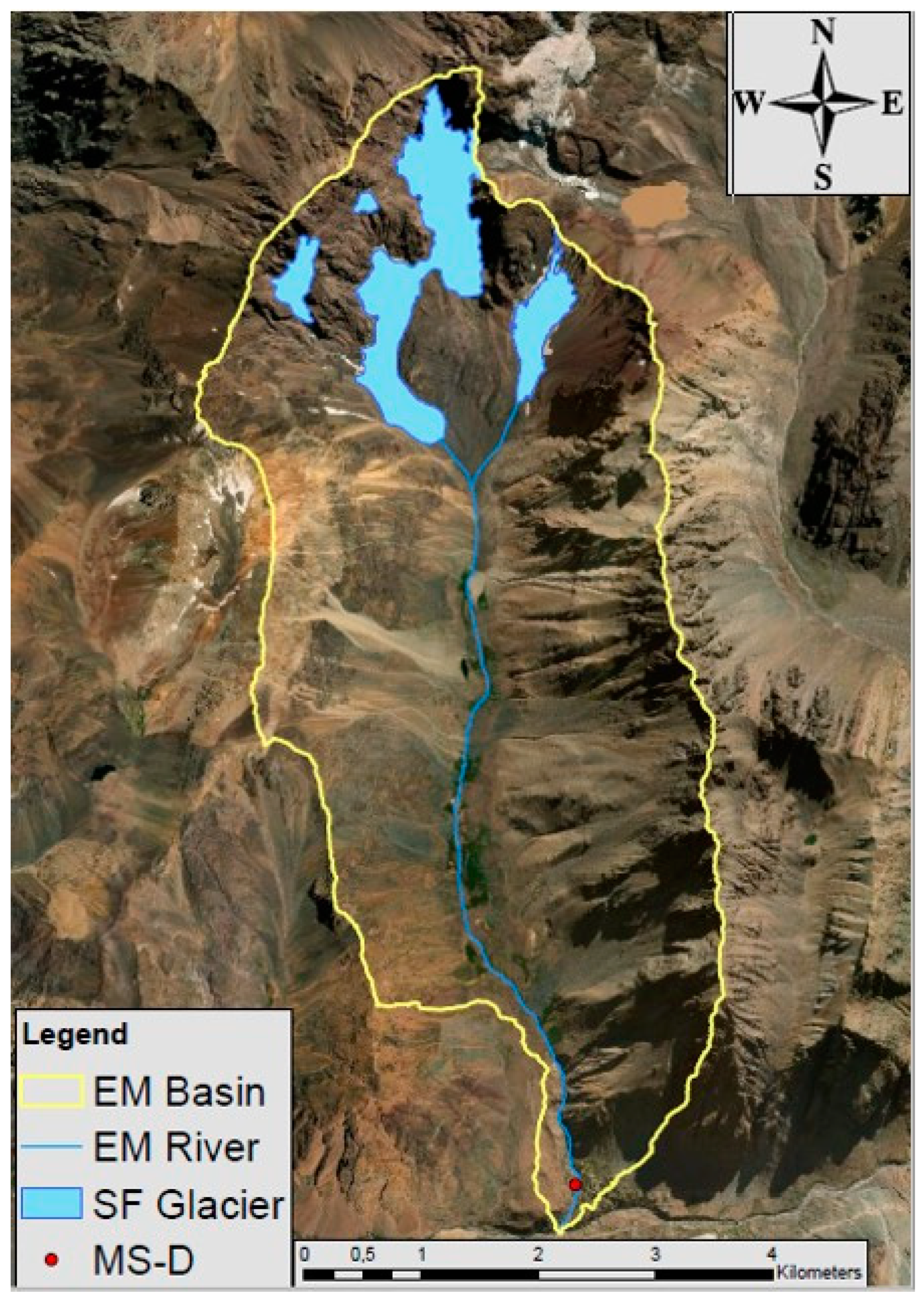
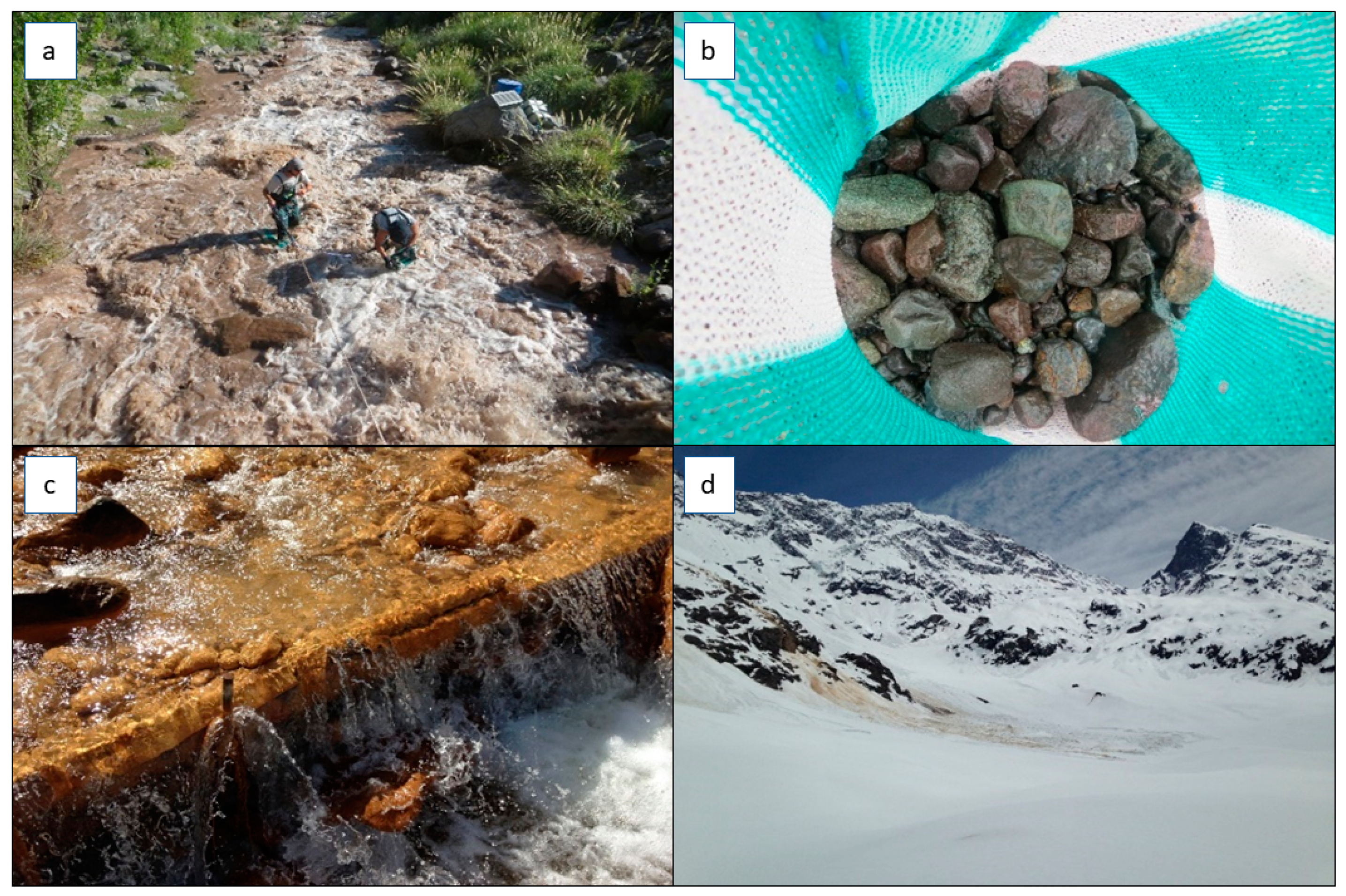
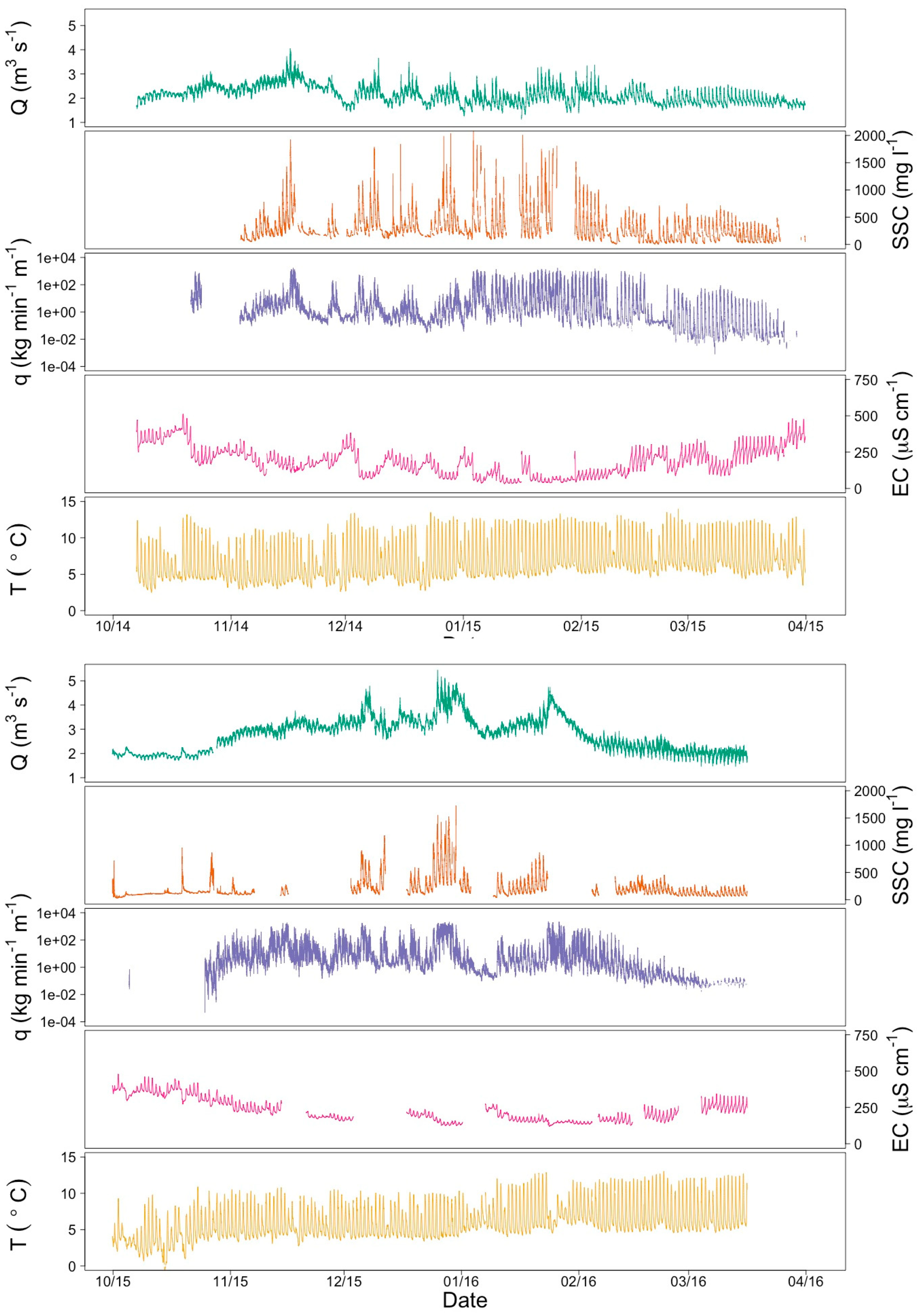
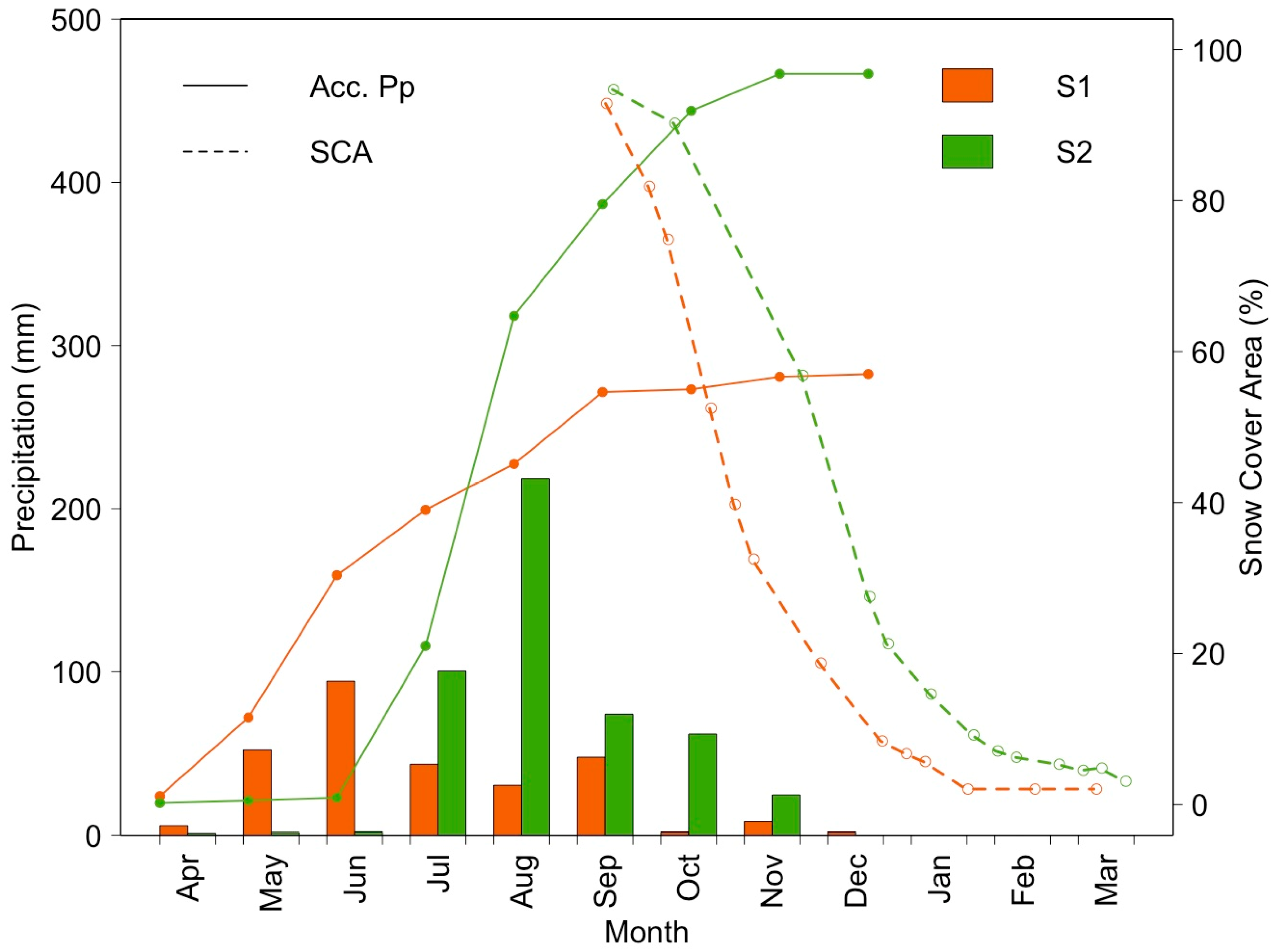
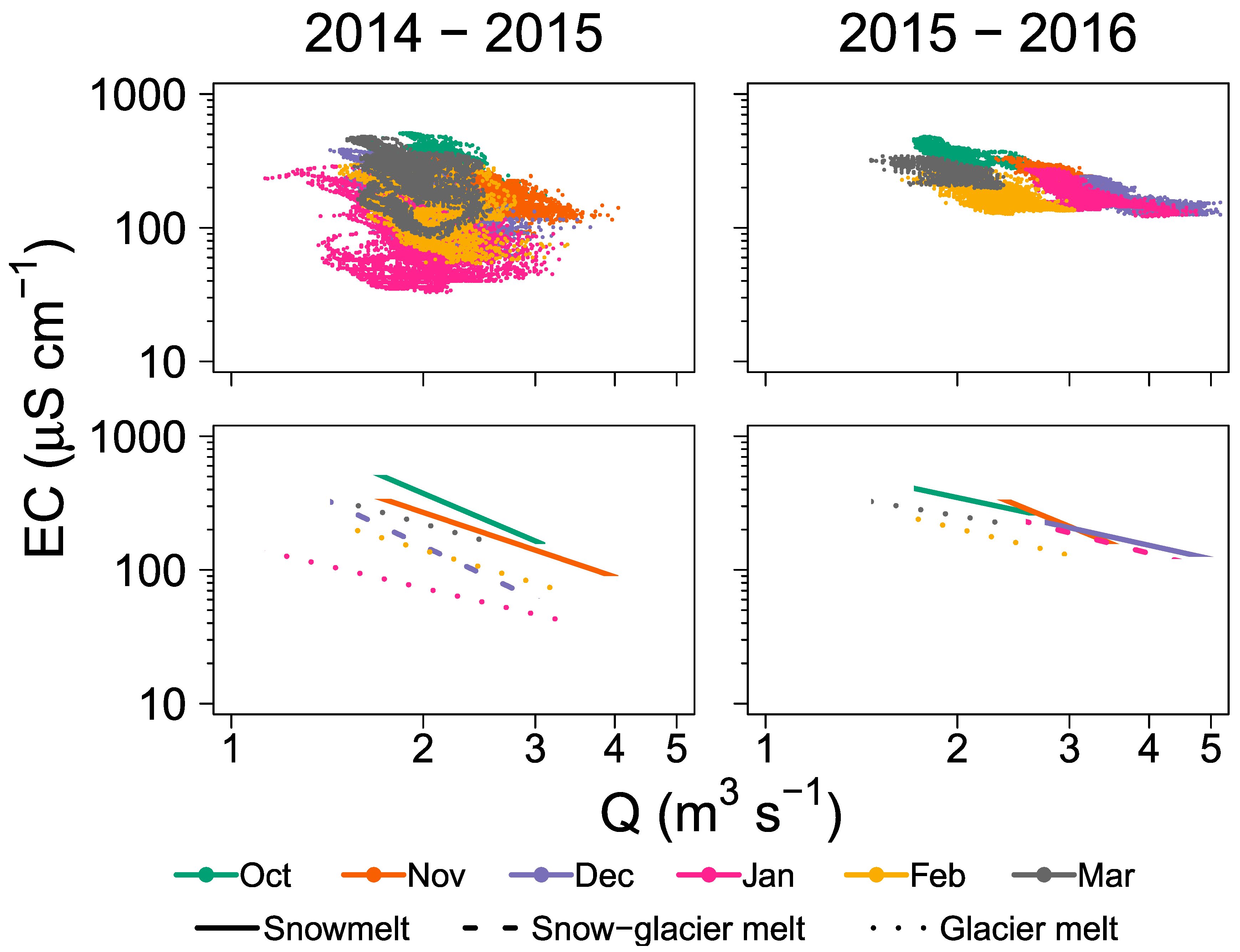
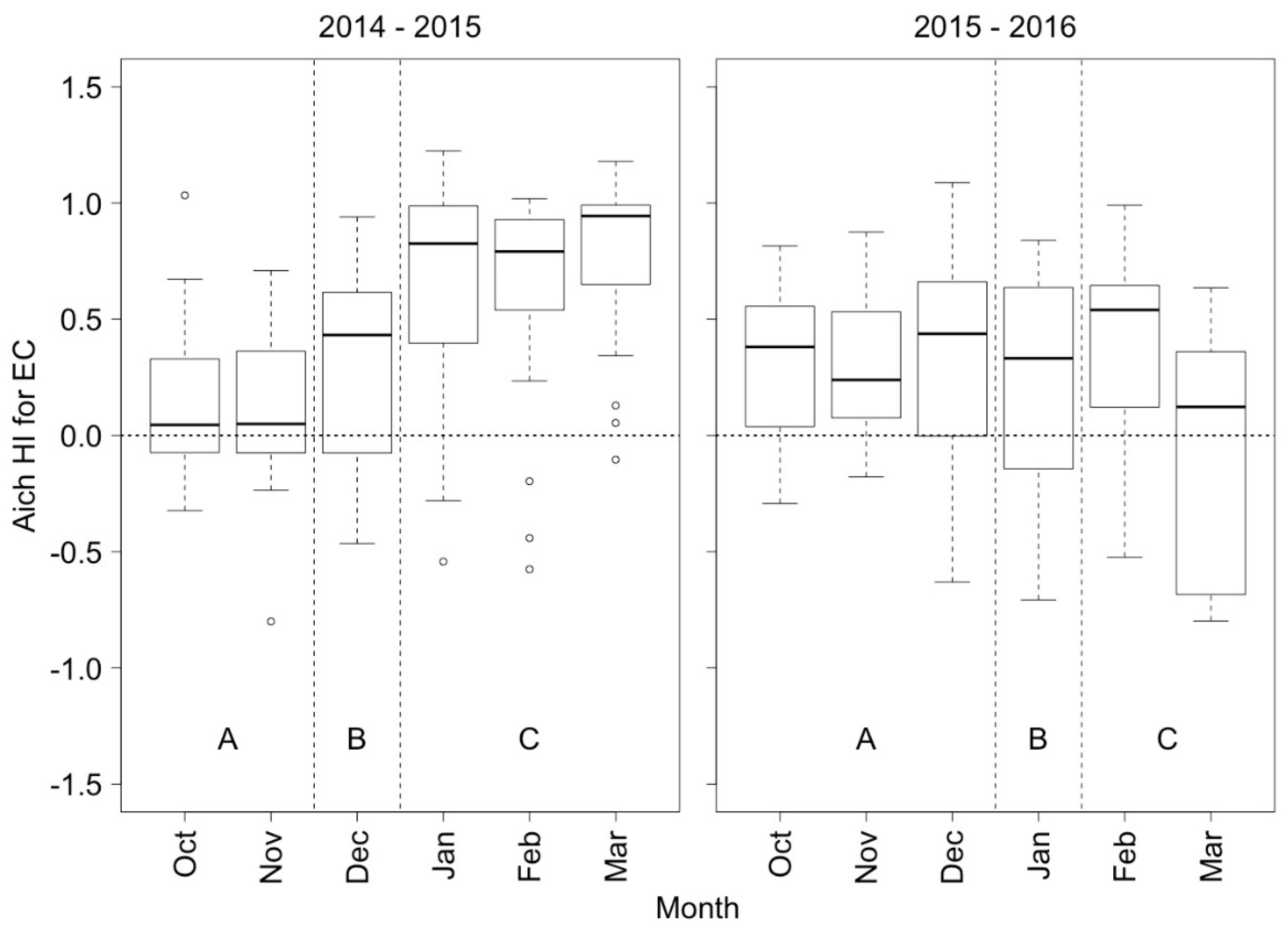
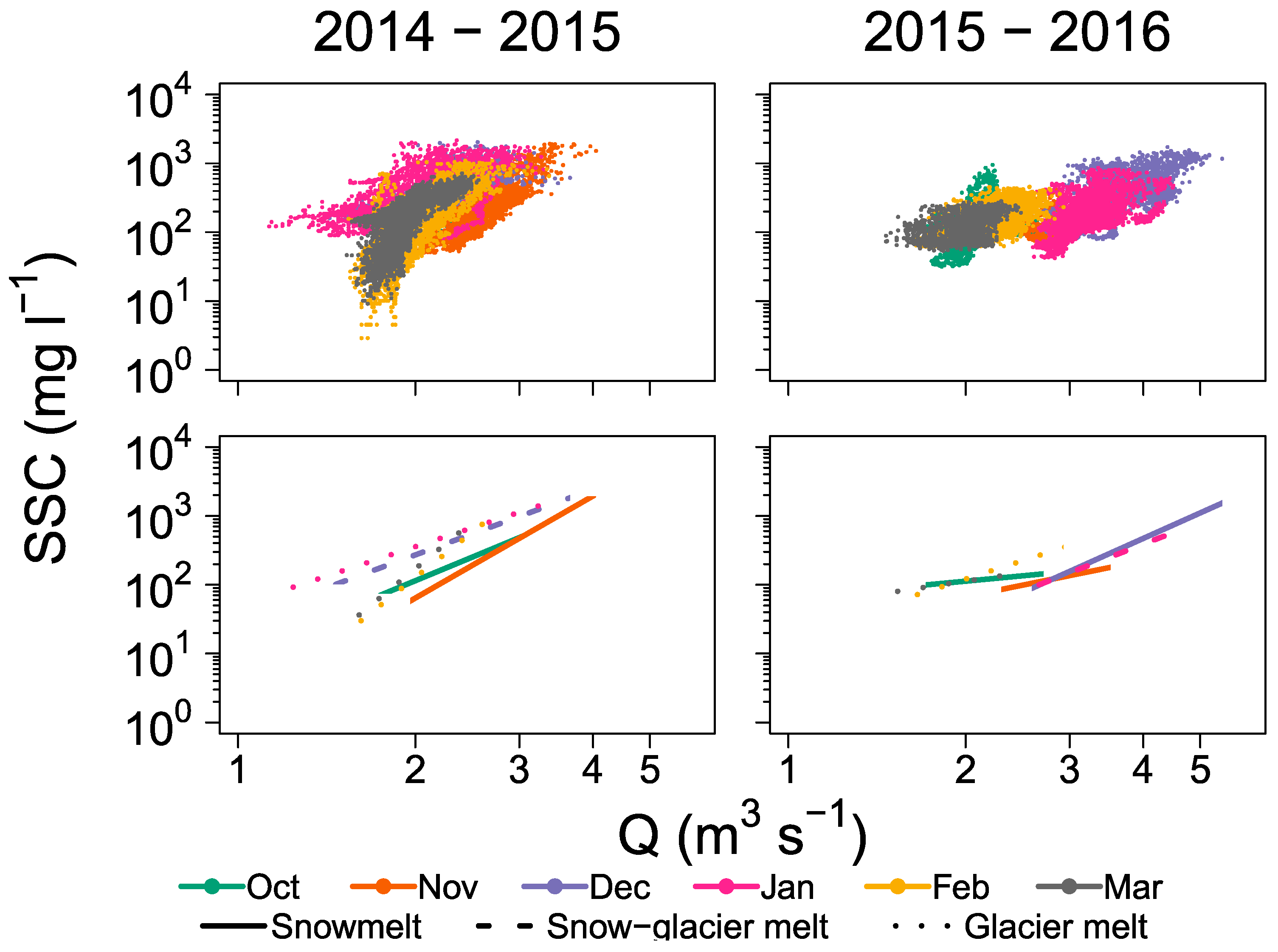
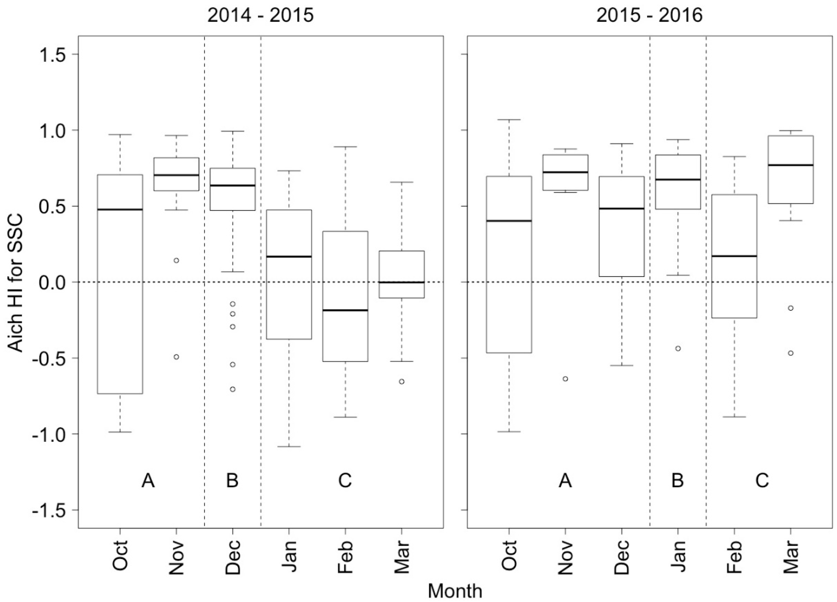
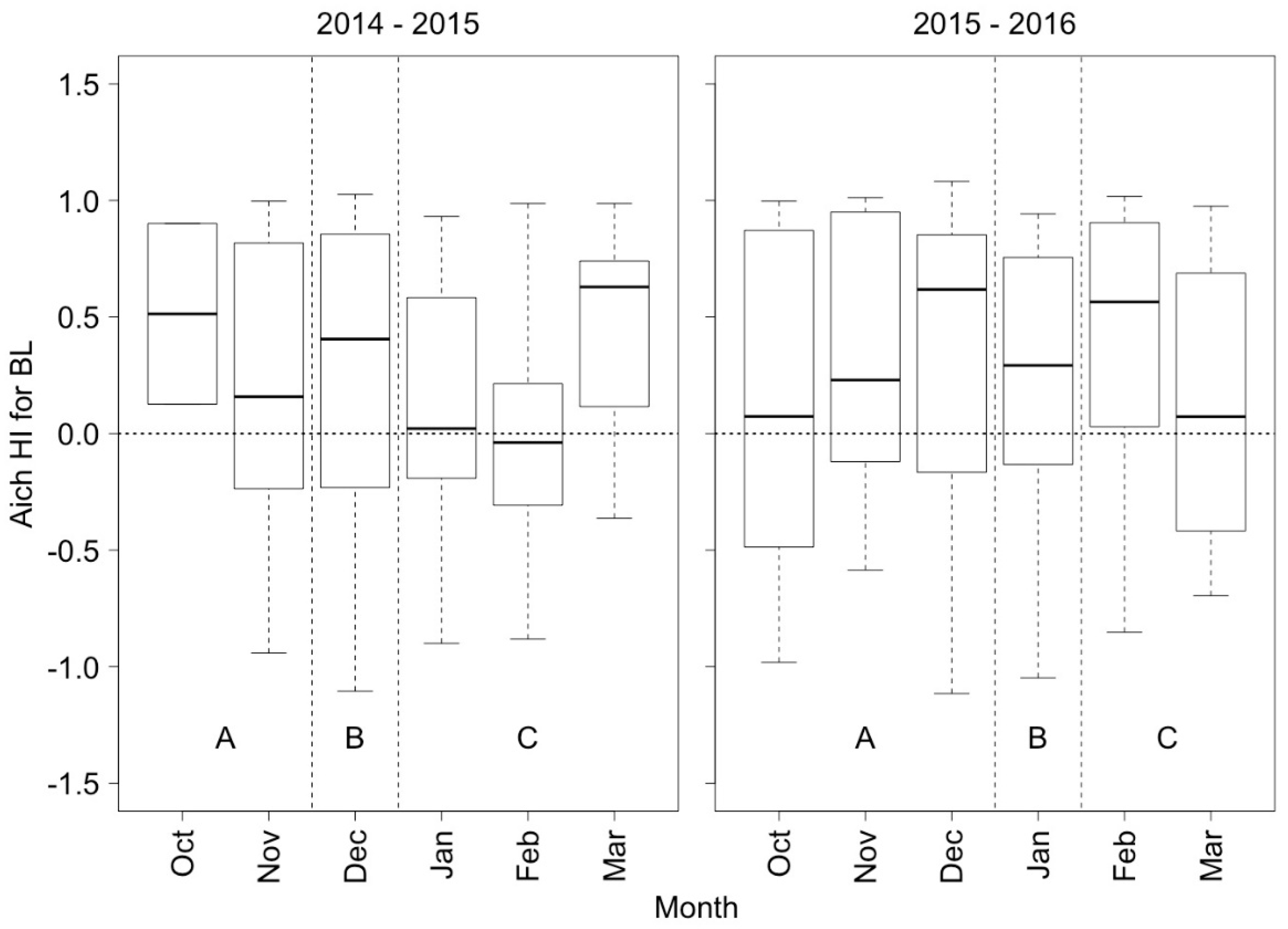
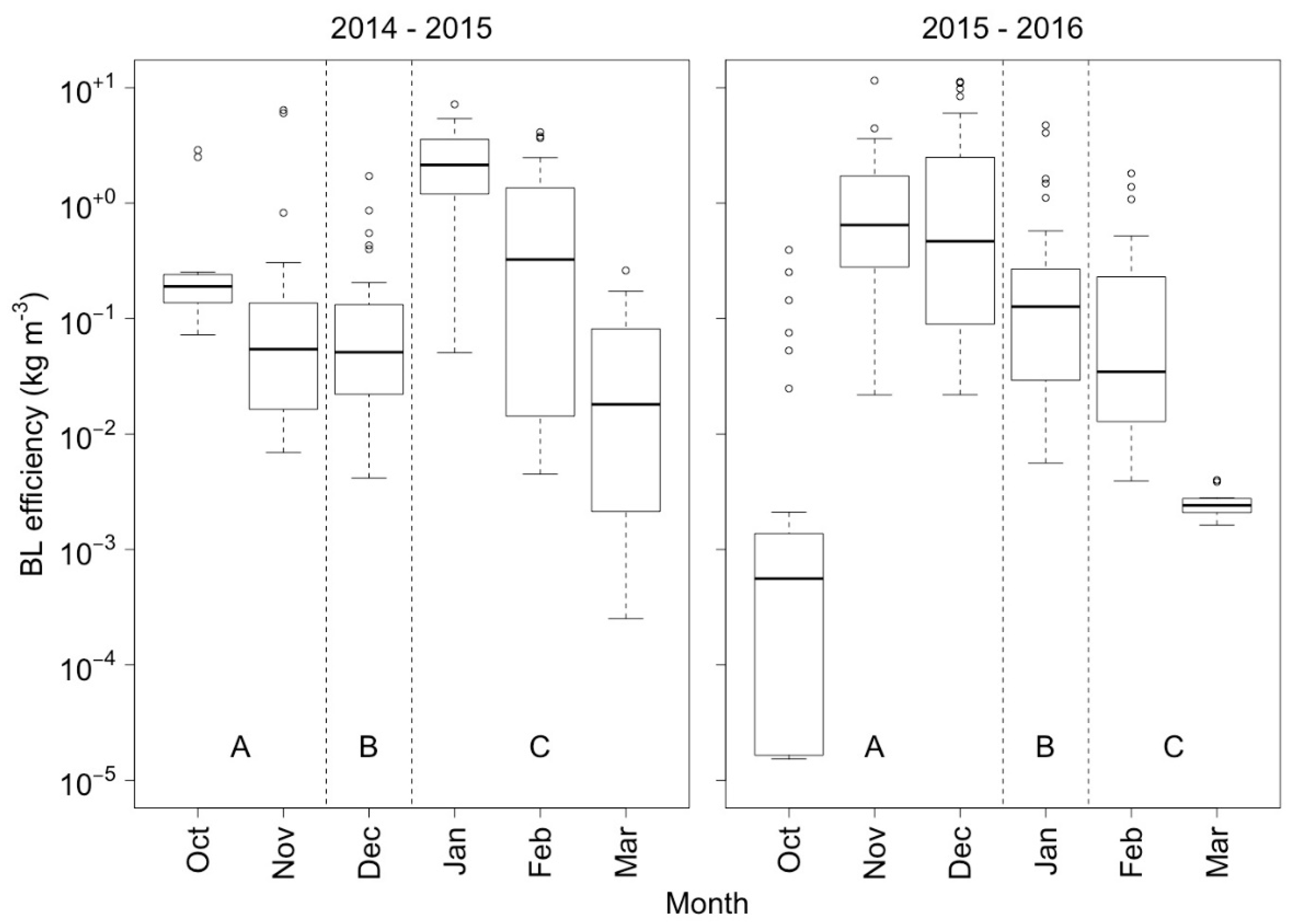
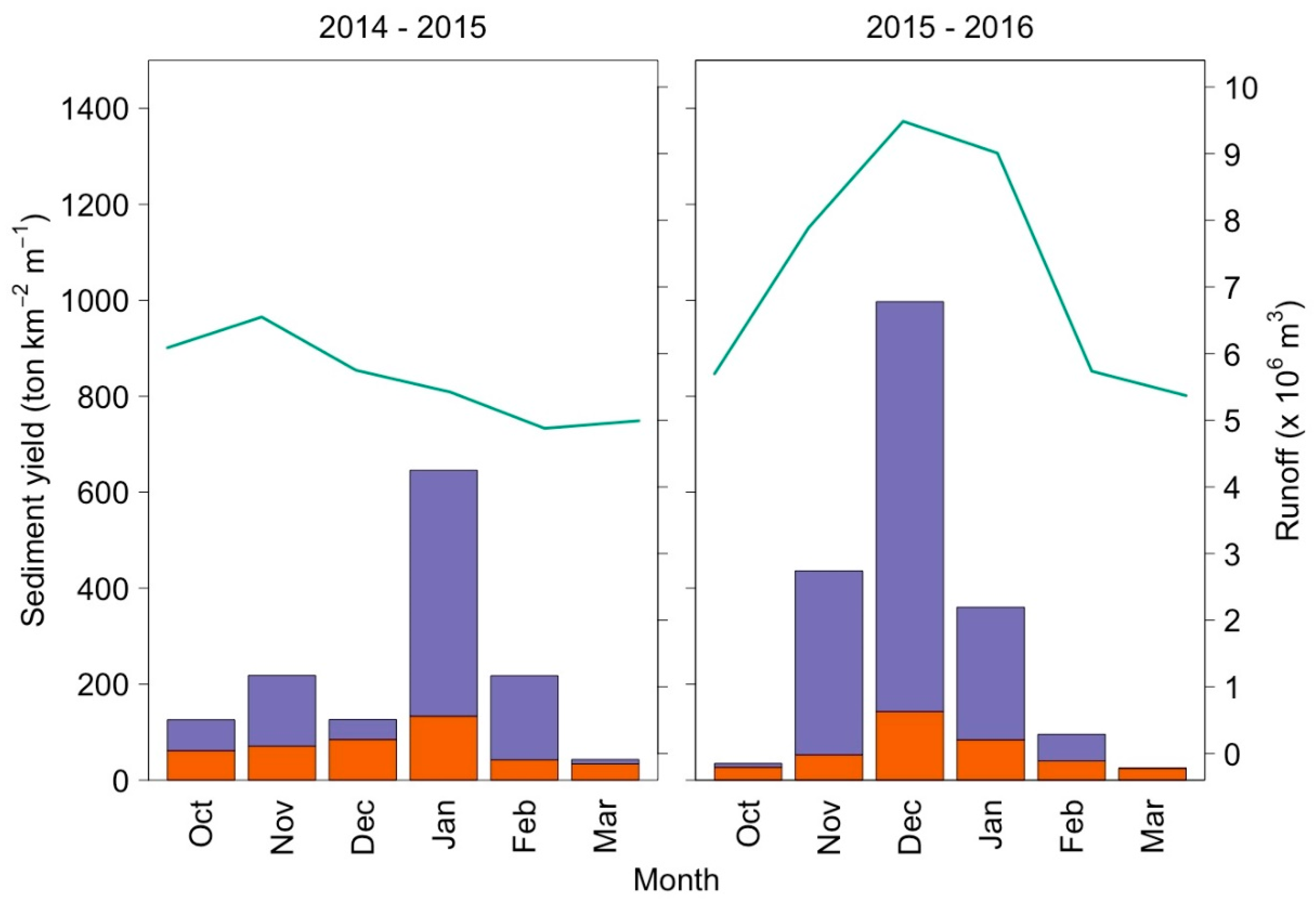
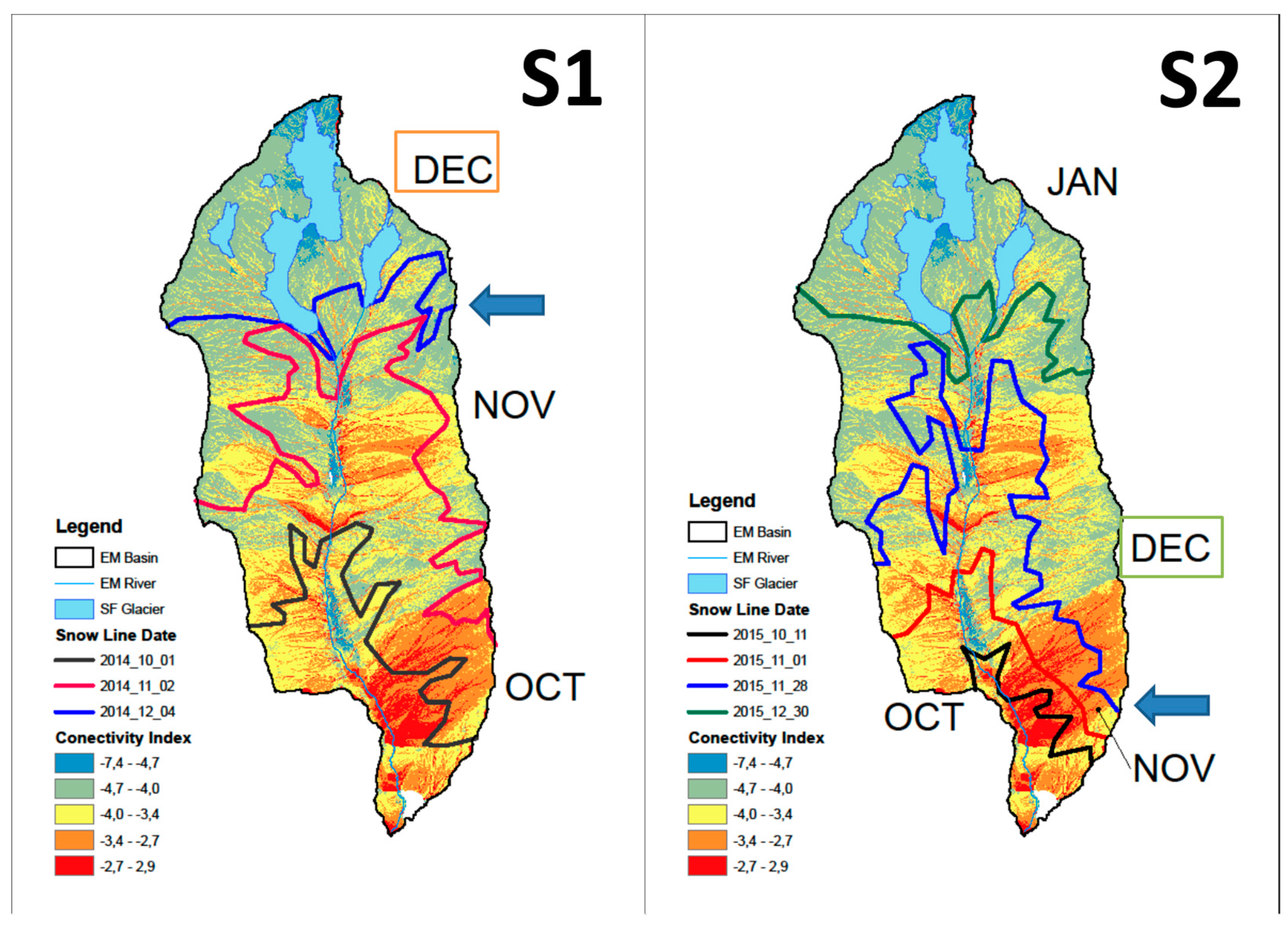
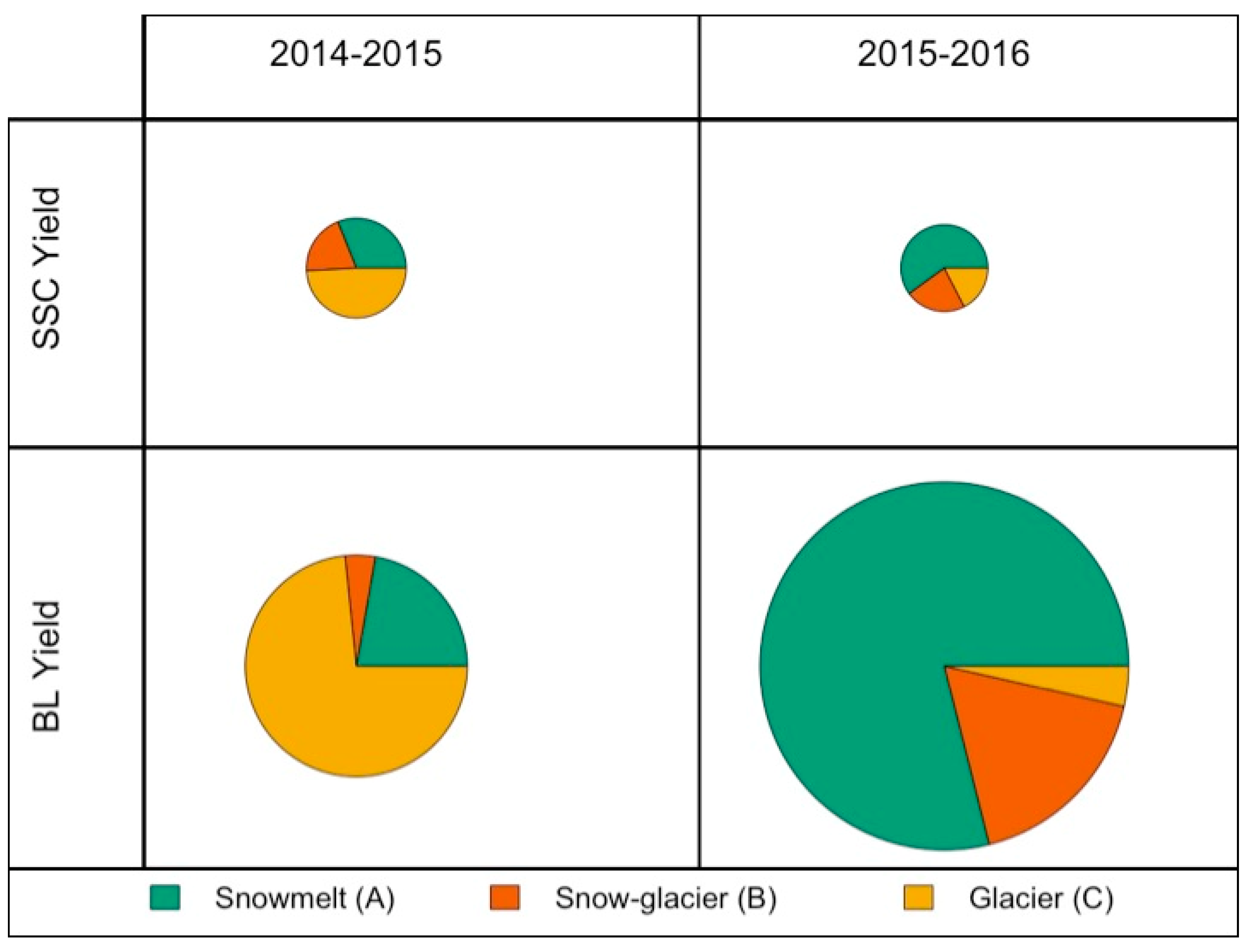
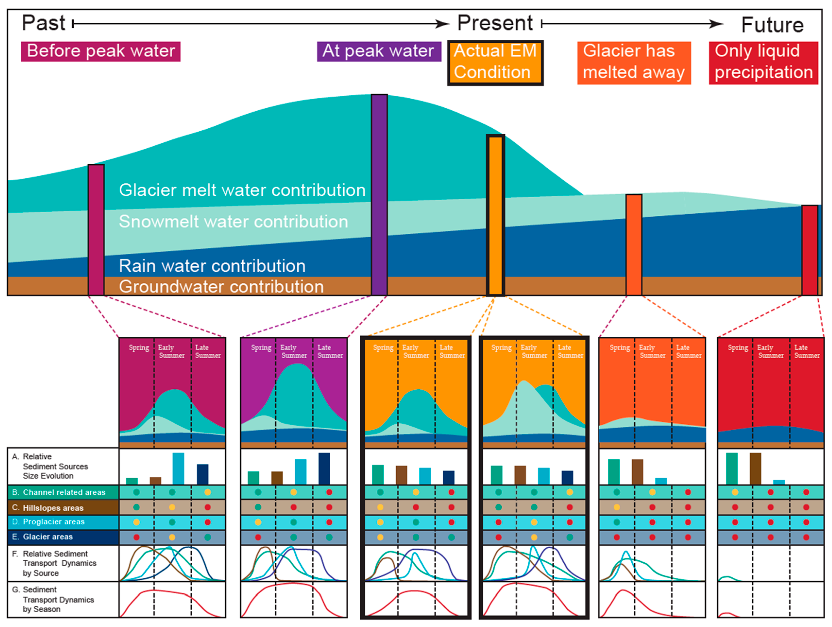
Table 1.
Periods in which the ablation season in the Estero Morales can be split, depending on the dominant origin of melting water. The main origin of runoff is split in snowmelt (A), snow and glacier melting (B) and glacier—later glacier melting periods (C).
Table 1.
Periods in which the ablation season in the Estero Morales can be split, depending on the dominant origin of melting water. The main origin of runoff is split in snowmelt (A), snow and glacier melting (B) and glacier—later glacier melting periods (C).
| Ablation Season | Snowmelt (A) | Snow-Glacier Melting (B) | Glacier Melting (C) | Late Glacier Melting (C) |
|---|---|---|---|---|
| 2014–2015 | October–November | December | January–February | March |
| 2015–2016 | October–December | January | February | March |
Publisher’s Note: MDPI stays neutral with regard to jurisdictional claims in published maps and institutional affiliations. |
© 2020 by the authors. Licensee MDPI, Basel, Switzerland. This article is an open access article distributed under the terms and conditions of the Creative Commons Attribution (CC BY) license (http://creativecommons.org/licenses/by/4.0/).
Share and Cite
MDPI and ACS Style
Carrillo, R.; Mao, L. Coupling Sediment Transport Dynamics with Sediment and Discharge Sources in a Glacial Andean Basin. Water 2020, 12, 3452. https://doi.org/10.3390/w12123452
AMA Style
Carrillo R, Mao L. Coupling Sediment Transport Dynamics with Sediment and Discharge Sources in a Glacial Andean Basin. Water. 2020; 12(12):3452. https://doi.org/10.3390/w12123452
Chicago/Turabian StyleCarrillo, Ricardo, and Luca Mao. 2020. "Coupling Sediment Transport Dynamics with Sediment and Discharge Sources in a Glacial Andean Basin" Water 12, no. 12: 3452. https://doi.org/10.3390/w12123452
Note that from the first issue of 2016, this journal uses article numbers instead of page numbers. See further details here.