Case Study: Reconstruction of Runoff Series of Hydrological Stations in the Nakdong River, Korea


1
Ministry of Environment, Han River Flood Control Office, Seoul 06501, Korea
2
National Territorial Environment & Resources Research Division, Korea Research Institute for Human Settlements, Sejong 30149, Korea
3
Institute of Water Resources System, Inha University, Incheon 22212, Korea
4
Department of Civil Engineering, Inha University, Incheon 22212, Korea
*
Author to whom correspondence should be addressed.
Water 2020, 12(12), 3461; https://doi.org/10.3390/w12123461
Submission received: 5 November 2020
/
Revised: 30 November 2020
/
Accepted: 1 December 2020
/
Published: 9 December 2020
(This article belongs to the Section Hydrology)
Abstract
:Reliable runoff series is sine qua non for flood or drought analysis as well as for water resources management and planning. Since observed hydrological measurement such as runoff can sometimes show abnormalities, data quality control is necessary. Generally, the data of adjacent hydrological stations are used. However, difficulties are frequently encountered when runoff series of the adjacent stations have different flow characteristics. For instance, when the correlation between the up- and downstream locations in which the stations are located is used as the main criterion for quality control, difficulties can occur. Therefore, this study aims to suggest a method to reconstruct an abnormal daily runoff series in the Nakdong River, Korea. The variational mode decomposition (VMD) technique is applied to the runoff series of the three target stations: Goryeong County (Goryeong bridge) and Hapcheon County (Yulji bridge and Jeogpo bridge). These runoff series are also divided into several intrinsic mode functions (IMFs) that are governed by basin runoff and disturbed flow caused by the hydraulic structure. The decomposition results based on VMD show that the runoff components in a particular station that is influenced by hydraulic structures could be reconstructed using adjacent stations, but the residual mode could not. The runoff reconstruction model using an artificial neural network (ANN), the two “divided” modes, and the residual component is established and applied to the runoff series for the target station (Yulji bridge in Hapcheon County). The reconstructed series from the model show relatively good results, with R2 = 0.92 and RMSE = 99.3 in the validation year (2019). Abnormal runoff series for 2012 to 2013 at the Yulji bridge station in Hapcheon County are also reconstructed. Using the suggested method, a well-matched result with the observations for the period from 2014 onwards is produced and a reconstructed abnormal series is obtained.
1. Introduction
The observation process plays a vital role in many studies and industries [1,2], and it is particularly important in hydrology and water resources management. Technological advances, such as real-time information acquisition or new measuring equipment, have been brought to a new level. However, there are still concerns about their use in practice. The microwave Doppler current meter (hereafter referred to as “MDCM”) [1,3], a new way to measure velocity or depth, has been found to be questionable in terms of reflectivity due to meteorological or structural conditions [4]. These erroneous and abnormal records sometimes mislead management, which often leads to property losses. Therefore, the accuracy of measurement should be ensured, especially in the field of hydrology and water resources management, where it is found to be a key issue [5].
Many studies contribute to reducing the error of measurements or suggest new methodologies which try to minimize systematic errors. For instance, the frequency of the MDCM was changed from 10 GHz to 24 GHz for efficiency [6,7]. The tracer method, which has been used for a long time to measure flow velocity, was also examined with various materials, including dye, salts, fertilizers, gases, and radioisotopes [8,9,10]. Sometimes, popcorn was even used for measurements [11] with the surface image velocimetry method [12]. On the other hand, some studies focused on error correction or the removal of uncertainty. Errors or uncertainties could be caused by the installation of the data acquisition system, the monitoring sensor interfering with accuracy, and abnormal jumping of instruments, among others [5]. The statistical approach is one of the most widely used methods to reconstruct abnormal data with precipitation [13,14], temperature [15], and runoff [16,17]. Spatial interpolation could be used for ground-level data [18] and gridded data [19], just the same as the CRESSMAN [20] or Barnes [21] methods. However, there are also studies wherein basic data quality control and reconstruction methods, such as logic, spatial, internal, and temporal interpolation and consistency checking, can detect anomalies but do not give a reliable value, because they fail to capture nonlinear characteristics and non-stationarity hidden in the hydrological series [22,23]. Therefore, advanced methods such as an artificial neural network (hereafter referred to as “ANN”) was widely employed to detect and correct abnormal data [24,25]. Machine learning techniques [26] are considered a good alternative to overcome the aforementioned existing limitations. The same goes for support vector regression (SVR), which is widely used to detect [27] anomalies or predict runoff series [28,29]. However, there is still difficulty when each runoff series has different flow characteristics [30]. Even though many studies and models could contribute to a more accurate reconstruction of abnormal data, such as regression [31,32], ANN [33,34], Adaptive neuro fuzzy inference system (ANFIS) [35], or a simplified weighted sum or average [36,37], all these methods need the same and inevitable assumption, that is, hydrological stations are stationary and correlated in the spatial or temporal scale (e.g., the up- and downstream stations). Thus, the above methods could not be applied when they have different flow characteristics from their adjacent stations [16].
The objective of the study is to suggest a method to reconstruct the abnormal runoff series in the observed data, which has different flow characteristics as compared to the adjacent hydrological stations. Some creative studies suggest that the runoff series could be divided into several components with local frequency ranges [38], and it could also be reconstructed by summing up each component [39,40]. Inspired by these studies, variational mode decomposition (hereafter referred as “VMD”) was employed to divide runoff series into several intrinsic mode functions (hereafter referred as “IMFs”) and residuals. A runoff reconstruction model was established using an ANN technique and was “divided” using IMFs and residuals of the 2014 to 2019 runoff series. Established models showed a well-matched result with the observed data and analyzed its efficiency and applicability. Using the model, the abnormal runoff series from 2012 to 2013 at the Hapcheon County (Yulji bridge) station were reconstructed.
2. Methods
2.1. Study Material
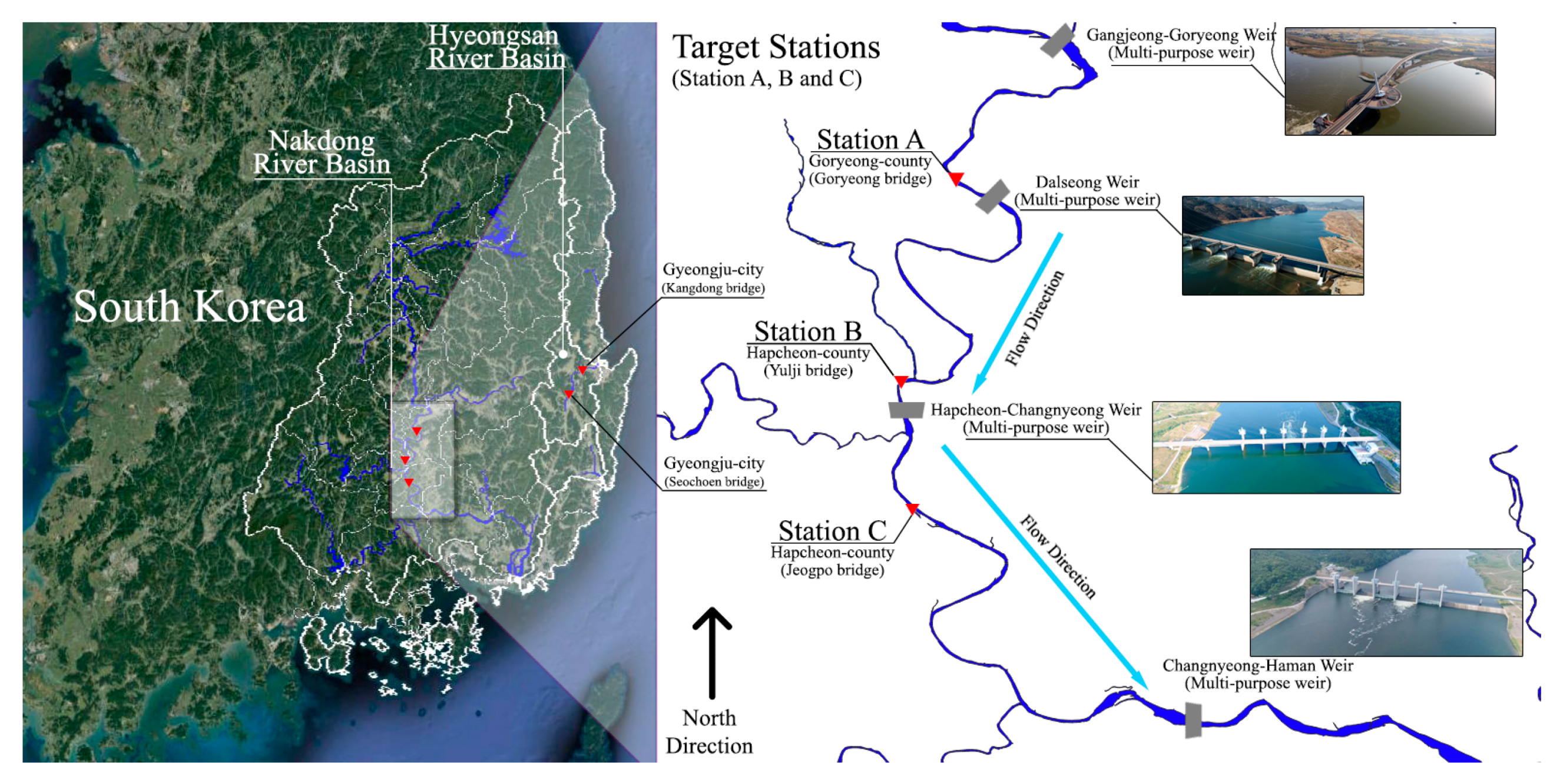
The target of the study are the three hydrological stations—Goryeong County (Goryeong bridge), referred to as station A, Hapcheon County (Yulji bridge), referred to as station B, and the main target of runoff reconstruction, Hapcheon County (Jeogpo bridge), referred to as station C—which were constructed in the middle of the main stream of the Nakdong River, as shown in Figure 1. All of them are adjoined and located in the upper to downstream zones along the 40 km river length. From these stations, the water level and runoff series were obtained. During the Four Major Rivers Restoration Project, many hydrological stations were constructed to collect essential data that are used to maintain the multi-purpose weir (dam) in the Nakdong River [41]. Almost all of them, including the targets of the study, employ automated measuring equipment, such as acoustic Doppler velocity meters (ADVMs) [42] to avoid disturbing the flow influence of the weirs. The upper-basin areas of the stations are 14,034, 15,053, and 16,449.6 km2 and the river widths at the stations are approximately 150 m, 350 m, and 550 m, respectively. The runoff amount at the median water level is 79.2, 93.4, and 101.0 m3/s for each station from 2014 onwards. The start year of the observations for each station was February 1968 for station A, February 2006 for station B, and June 1980 for station C. However, flow characteristics were significantly changed by the Four Major Rivers Restoration Project [43], which caused the unmatched historical record of runoff from 2012 to the present. Table 1 shows the general flow conditions and changed characteristics before and after the project. Overall, the flow amount of each quantile was approximately increased by 10~20 m3/s, and the kurtosis coefficient, which is highly correlated with the shape of distribution, was also increased. Stations A, B, and C are considered to be very important points due to being: (i) runoff observatories in the middle part of the Nakdong River, (ii) validation points of the inflow amount from the Hwang River, which is one of the main tributaries, and (iii) the official check points for green algal blooms of the Nakdong River [43]. So, all of them are essential for water resources management, including flood, drought, and water quality. However, station B has abnormal data from 2012 to 2013 that show approximately 3200 m3/s for the average runoff amount, despite stations A and C showing averages of 208 m3/s and 259 m3/s, respectively. So, the historical runoff record of 2012 to 2013 is insignificant and the official approval of hydrological data for the target stations has not been implemented due to the runoff consistency problem. The daily runoff series data of the three hydrological stations and their properties were obtained from the Water Resources Management Information System [44].
2.2. Variational Mode Decomposition (VMD)
VMD was developed by Dragomiretskiy and Zosso (2013) [45] to overcome the limitations of empirical mode decomposition (hereafter referred to as “EMD”) [46]. In principle, all of the “mode decomposition” techniques are used to decompose a signal into several fast and slow oscillating components, which are called IMFs, or simply, “mode”. It enables breaking through the limitation of traditional harmonic analysis, which is based on the Fourier transform [47]. However, there is also a mode-mixing problem, which has been defined as the IMF consisting of oscillation frequencies of disparate scales which makes the decompositions harder to interpret [48]. VMD aims to decompose a signal into k band-limited modes with specific sparsity properties [45]. The constrained variational formulation for yielding the IMFs can be expressed as follows:
where and are the th mode and its center frequency of signal, respectively. and are shorthand notations for the set of all modes and frequencies, denotes the Euclidean distance (), is the Dirac distribution, denotes convolution, is the Fourier transform of the signal , is the amount of data, is the time step, and is original signals. Equation (1) is changed to the following unconstrained equation by introducing an augmented Lagrangian [45].
where denotes the balancing parameter, is the Lagrange multiplier, is the scalar product, and Equation (2) could be solved with the alternate direction method of multipliers (ADMM) [49]. Additionally, the mode can be obtained using:
where is the Fourier transform of the signal , is understood as the inverse Fourier transform, and is the real parts of the signal. Equation (3) has a Wiener filtering structure, so, the mode in the time domain can be obtained from the real part of the inverse Fourier transform. More specific details on VMD and its process can be found in Dragomiretskiy and Zosso (2013) [45], and Herrera et al. (2014) [45,50].
2.3. Artificial Neural Network (ANN)
There are many models and techniques to forecast or simulate and reconstruct hydrological series. An ANN was treated as a good alternative because it had shown an ability to reproduce and capture nonlinearity in pattern recognition [51,52], signal classification [52,53,54], trajectory prediction [54,55], and even financial trading [53,56]. Additionally, an ANN could be regarded as a better option than Autoregressive integrated moving average (ARIMA) or Autoregressive (AR)-related models in forecasting or simulating seasonal time series [57] and reconstructing nonlinear time series, including runoff [22,23]. Therefore, an ANN is found to be a suitable method to reconstruct runoff series using the IMFs that were decomposed by VMD.
The ANN mimics the structure and connectivity and functions of nodes through which neurons are connected to each other in biological systems [58]. Generally, an ANN is composed of three layers: the input layer which represents the observed data, the output layer which serves as the result of reconstruction, and the hidden layer which is a network of neurons trained to recognize observed data [59]. The back-propagation algorithm has been used in the structure to train the connection strength to learn about the error and optimize the neurons, therefore, an appropriate algorithm is essential for ANN modeling [60]. The Levenberg–Marquardt–QNBP algorithm was selected as the back-propagation algorithm in accordance with its well-founded performance for nonlinear hydrological series [60].
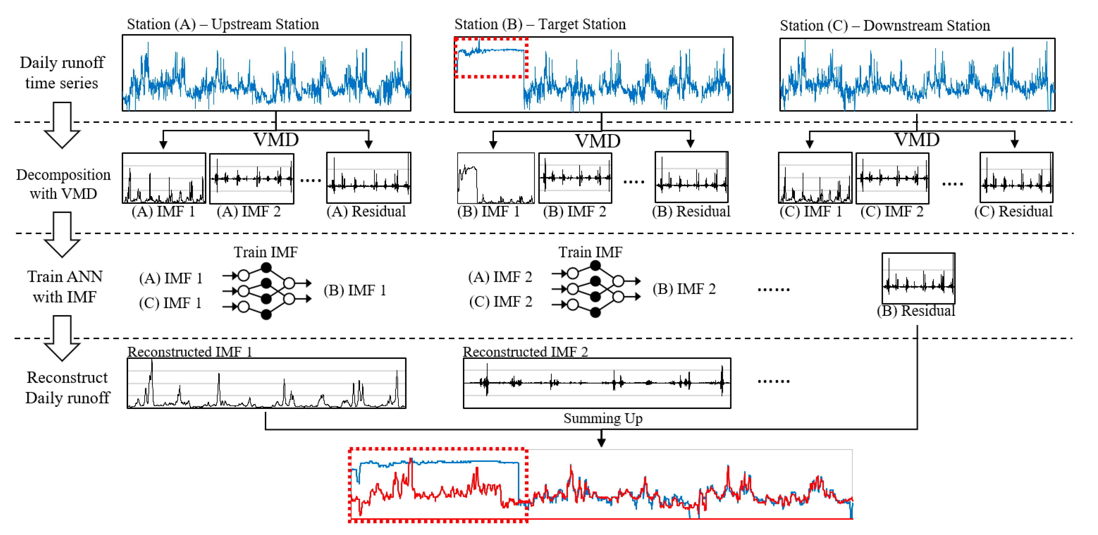
Finally, Figure 2 shows the overall framework and process for the runoff reconstruction model with three stages: (i) decomposing the runoff series into IMFs based on the VMD technique, (ii) training and establishing an ANN model to reconstruct each IMF using adjacent stations, and (iii) runoff reconstruction by summing up reconstructed IMFs and residuals.
3. Application and Discussion
3.1. Runoff Series Characteristics and Its Decomposition
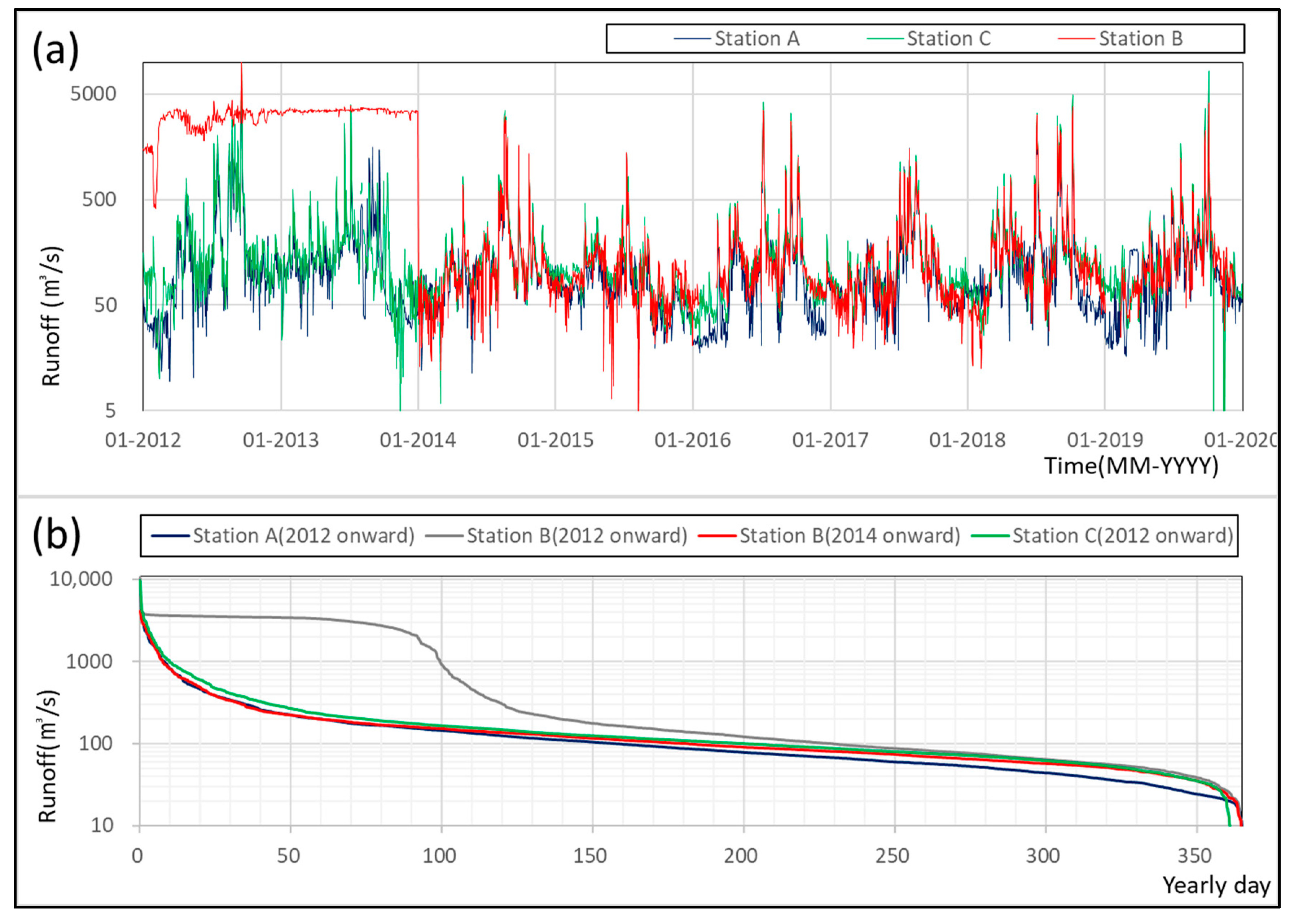
Figure 3 shows the obtained runoff time series from 2012 to 2019 and the abnormal data from 2012 to 2013 in station B. All of stations have a similar trend in the flow duration curve (FDC), except station B, including 2012 to 2013. It is assumed to have interference and instability during the period of stabilization. In fact, several hydrological stations in the Nakdong River showed the same problem. There are eight hydraulic structures (multi-purpose weirs) in the main stream, and the flow characteristic or correlation between each hydrological station is disturbed. For example, adjacent hydrological stations in the Hyeongsan River—specifically, Gyeongju City (Seochoen bridge) and Gyeongju City (Kangdong large bridge) in Figure 1—showed 0.94 for the correlation coefficient from 2012 to 2019 (See Figure 4a). In stark contrast, stations A and B (see Figure 4b) and B and C showed only about 0.49 and 0.55 for the correlation coefficient in the same period despite similar distances in between stations (km) and times of concentrations [61].
One of the challenges in the target stations is the quality control for abnormal or missing data. All of the observed data cause concerns about their general use in practice due to their accuracy, with abnormal and missing data during the observation process. Different flow characteristics tend to make quality control more difficult because the techniques to fill or adjust hydrological data depend on the correlation between adjacent hydrological stations. For instance, Figure 4a shows a relatively constant correlation for the Hyeongsan River, unlike in Figure 4b, wherein there are two groups of correlations which make it hard to determine the exact correlation between the two stations. In this case, it is difficult to fix the abnormal data. This is the reason why the data in station B from 2012 to 2013 cannot be solved (see Figure 3) and why VMD was selected and applied for the study.
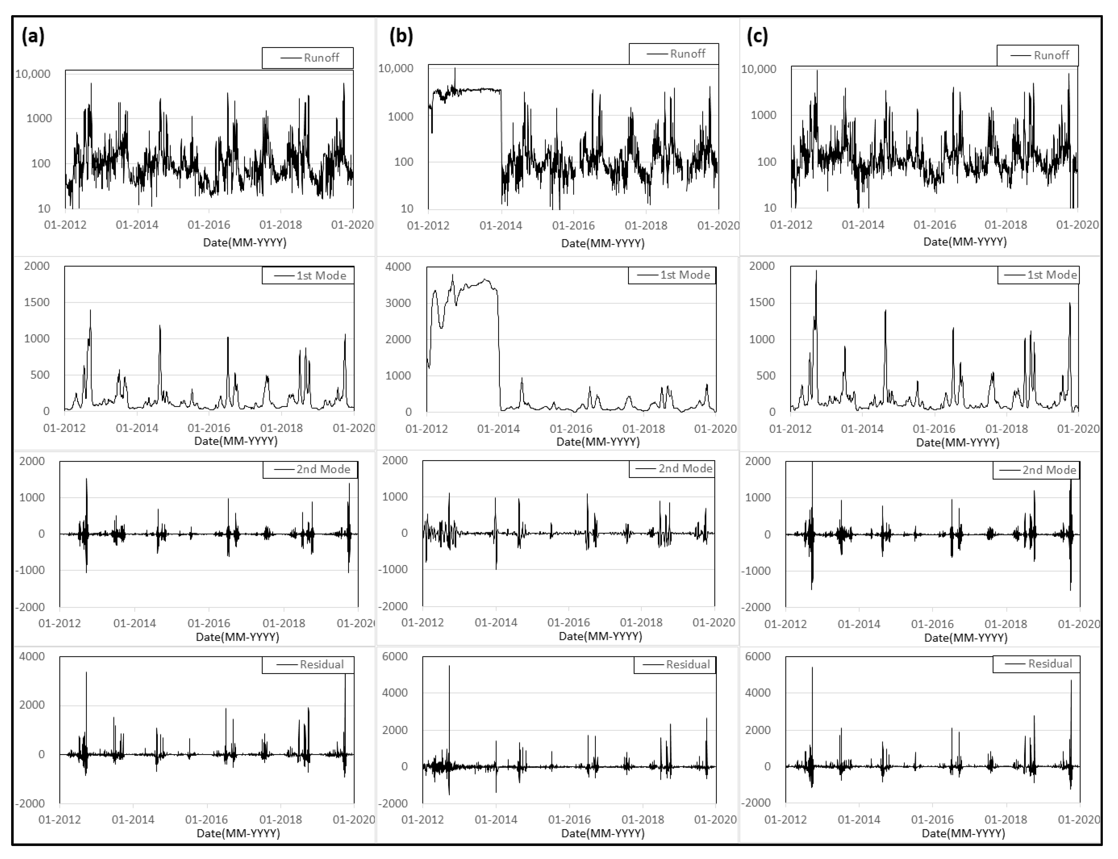
Since VMD can decompose a signal into several numbers of each oscillating component [45], it could be used as a method to divide runoff series into several “correlated” and “independent” components with their own frequencies, and it can also be used as basic data to reconstruct or predict runoff series [39]. Therefore, VMD was applied to the runoff series of the target stations (see Figure 5). Each series was decomposed into two IMFs (1st mode, 2nd mode) and a residual mode. The parameters of VMD, such as the moderate bandwidth constraint, were calibrated with trial and error, focusing on the simulated efficiencies of hydrological series because there are no criteria to select the exact value for the hydrological series. The decomposed result of each runoff series shows fascinating results in Figure 5a–c: (i) the 1st and the 2nd mode showed a similar trend which, during the calibration process, have correlation coefficients of 0.90, 0.88 for stations A and B, and 0.91, 0.78 for stations B and C, respectively. The station B series from 2012 to 2013 has inaccurate observations due to the facility issue. (ii) The residual shows a less similar trend for whole periods, with a value of 0.75 or less for stations A and B and C for correlation coefficient, and (iii) stations A and C show “very” similar trends, with 0.96, 0.95 for 1st, 2nd mode, and 0.76 for the residual in the correlation coefficient for the whole period. Therefore, some conclusions could be reached by combining these results since there are common components for all of them, and it could be assumed to be rainfall–runoff processes of the basin. Both show a very similar trend with over 0.9 or more in the correlation coefficient, which means that these modes are governed by the same components or local frequency ranges [39]. Therefore, the 1st and 2nd modes are runoff components and entirely governed by rainfall–runoff processes. Furthermore, the residuals are probably a mixture of runoff components and their own flow characteristics, such as back-water, disturbed flow, and other uncertainties. The residual shows a constant value in the correlation coefficient, with 0.75 or less regardless of the periods or stations, but not for the modes. This could be due to a mixture of the same and different characteristics with local frequency ranges [38]. Therefore, the 1st and 2nd mode could be used as the data to explain the runoff series in other stations, but the residual could not be used.
3.2. Establishment of Reconstruction Model
The 1st and 2nd modes could be used to explain others, but the residual could not. Thus, the two modes could be a target of “reconstruction”, but the residual should only be used for itself. Therefore, to fill the abnormal data from 2012 to 2013, the 1st and 2nd modes of station B were reconstructed using stations A and C, and the residual of station B was added to the reconstructed series to take into account its own flow characteristics. An ANN was employed to reconstruct the modes of station B due to its ability to capture the nonlinearity of the runoff series [62,63]. Since the runoff series has nonlinearity characteristics [64,65,66,67], an ANN will be a good alternative during the reconstruction process. Additionally, the number of hidden layers, which significantly affects whole ANN procedure, was set to 12 with trial and error, and the Levenberg–Marquardt–QNBP algorithm was selected as the back-propagation algorithm in accordance with its well-founded performance for nonlinear hydrological series [60]. Before the training process, all of the IMFs were normalized to improve the efficiency of the ANN model and avoid large fluctuations during the training process [39]. The normalization formula is defined as follows:
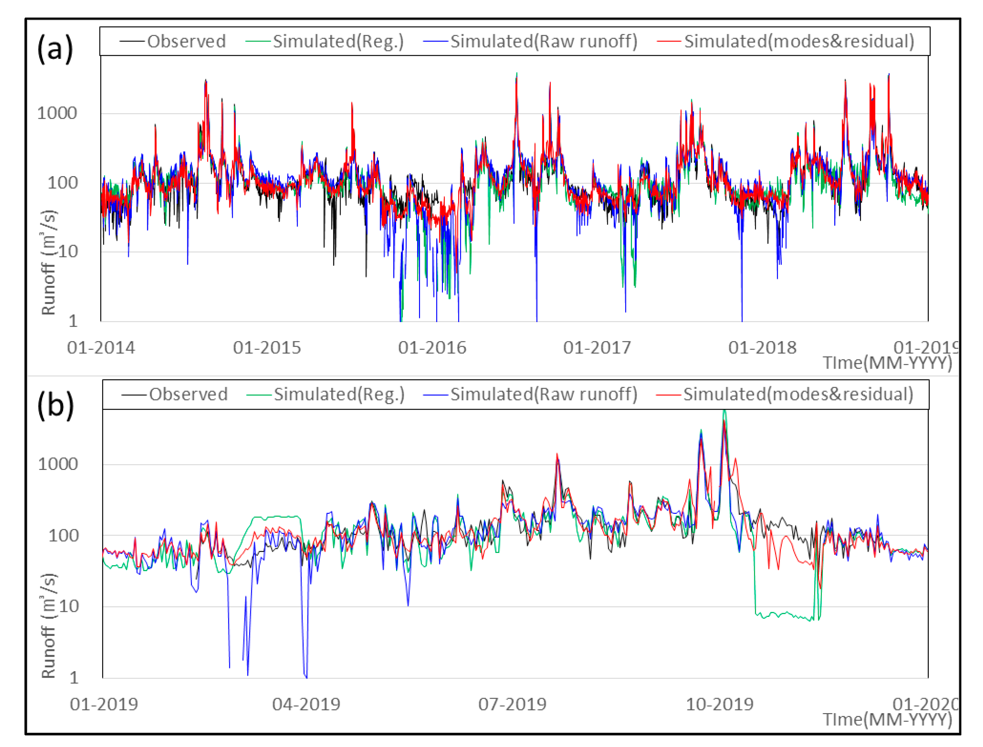
where is the normalized IMF, is the original IMF, and are the maximum and minimum value of the IMF, respectively. To validate the performance of reconstruction, the 1st and 2nd modes from 2014 to 2019 were divided into two periods: 2014 to 2018 for training and 2019 for validation. Another ANN model using raw runoff series was also established to compare with the suggested method of the study. Both of them had the same parameters, input periods, and algorithm, the only difference between the two ANN models was the data, wherein one used modes and residuals while the other used raw runoff series. Additionally, multiple regression, which is widely used to reconstruct missing or abnormal data, was employed as one of the control groups (see Figure 6 and Table 2).
Comparison results are shown in Figure 6a,b and Table 2. To sum up, both ANN results look like more convincing performances than multiple regression. For learning periods, the ANN with VMD has 0.93, 80.3 for the coefficient of determination (R2) and root mean square error (RMSE), which are widely known and used as measures and evaluation for model performance or selection criteria [68]. In comparison, the ANN with raw runoff and multiple regression has 0.93, 0.88 for R2 and 59.3, 116.7 for the RMSE, respectively. Therefore, both ANN models showed similar and better performance than multiple regression. Station B has 15,053 km2 of upper basin area and 350 m of river width, therefore, the station measures the runoff from a relatively large basin. It would be reasonable to regard it as an abnormal observation when station B shows a low flow rate of approximately 20 m3/s or less [61]. Having too little runoff is a problem in observation. The ANN with raw runoff and multiple regression shows several relatively small runoffs during both periods, such as 0.1–1.0m3/s in September 2015, 0.5–8.0 m3/s in August 2016, and 1.0–7.2 m3/s in March 2017. Station B has 51.8 m3/s at the drought water level, which is equal to 0.97 in percentiles [41]. Approximately 24 m3/s or less of runoff amount, which is 0.995 in percentiles in station B at the drought water level and is the confidence boundary for proper observation percentiles [69], has the probabilities of abnormal observation. In the periods of validation (2019), the ANN with raw runoff and multiple regression shows 0.84, 0.81 for R2 and 127.3, 219.2 for the RMSE, respectively. The ANN with VMD shows a more stable result with 0.91 for R2 and 99.3 for the RMSE. Above all, it does not show an abnormal trend or too little runoff during the whole period. Therefore, the suggested method based on VMD shows its applicability.
3.3. Reconstruction Results and Discussion
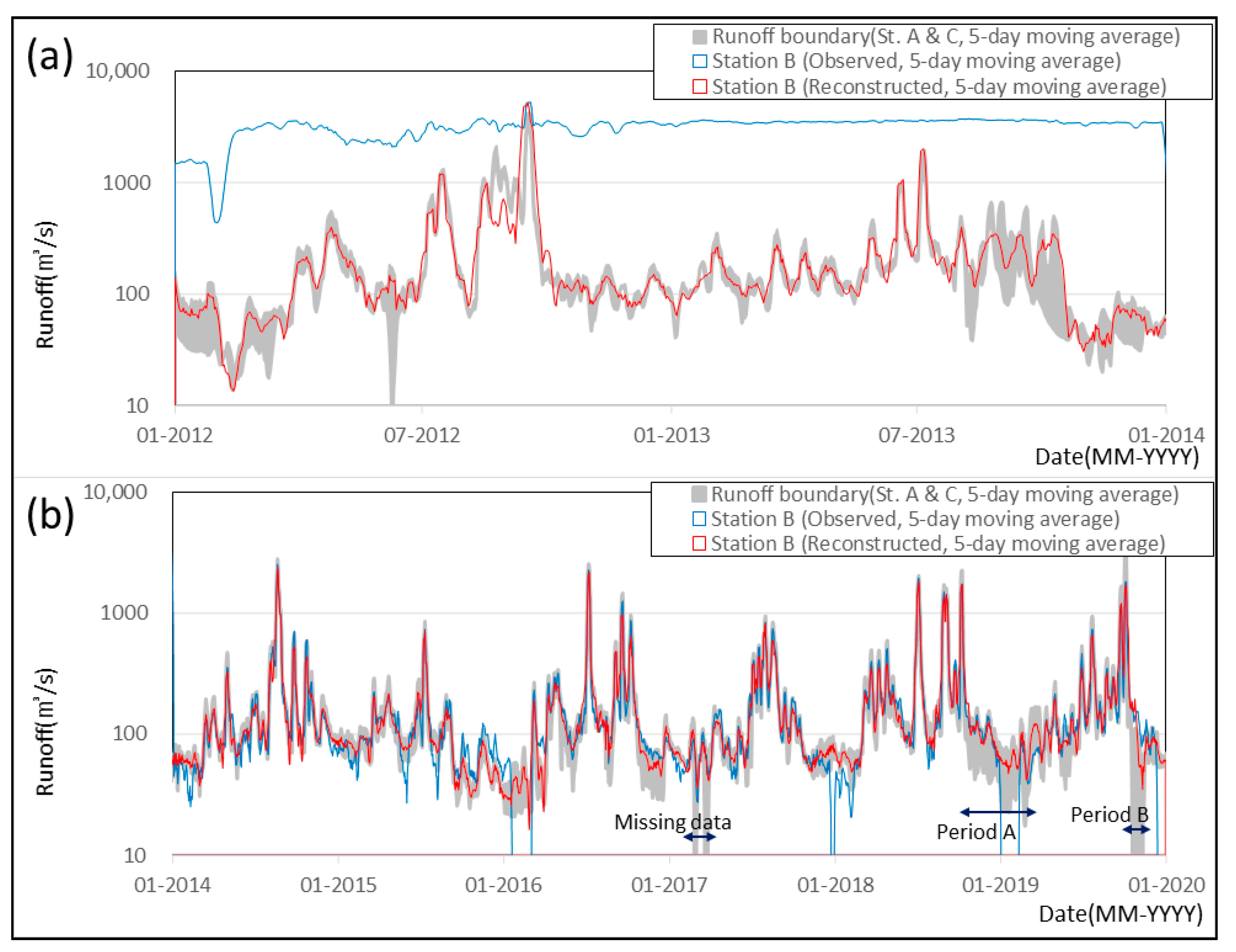
The abnormal runoff series from 2012 to 2019 in station B were reconstructed using an established ANN model with VMD, and its results are shown in Figure 7. For their visibility, reconstructed and observed runoff values are expressed as a 5-day moving average, and the runoff boundary, which is explained with high and low runoff values of stations A and C, are also plotted to compare with station B.
Overall, the reconstructed runoff series in station B has shown a relatively good result, with 0.92 for R2 and 55.9 for the RMSE from 2014 to 2019 (Figure 7b). Additionally, the reconstructed runoff series was identified to have the same distribution as the two-variable Kolmogorov–Smirnov test with a 95% significance level [70]. Of course, there is no “true value” of observations for 2012 to 2013, but the reconstructed series (red line) seems to be well matched with the observed runoff (blue line) after 2013. In fact, the reconstructed series shows a similar trend with the runoff boundary in stations A and C. Additionally, other evidence could be found in 2014 to 2019. In Figure 7b, there are three periods with wide range of runoff boundaries and abnormal runoff observations in station B: (i) the period (marked as “Missing data”) during March 2017 has a zero value of runoff in station A and was identified as missing data due to the failure of measuring equipment, (ii) period A during November 2018 to February 2019, with approximately a 65.0 m3/s difference with stations A and C and abnormal runoff (minus runoff value) in station B, and (iii) period B during October 2019, with approximately a 81.6 m3/s difference between stations A and C and abnormal runoff (1.0–10 m3/s) in station B. Technically, there is a relatively more constant low runoff amount in station C than stations A and B, therefore, it is insignificant since station C is the downstream station. Station C is located about 7 km downstream from the Hapcheon-Changnyeong weir and about 35 km upstream from the Changnyeong-Haman weir, and therefore it was influenced by the weirs (see the Figure 1). The Korean government established and carried forward the plan that tries to open and monitor the multi-purpose weir for environmental restorations (the Ministry of Environment 2019) [43]. As part of the plan, the Hapcheon-Changnyeong and Changnyeong-Haman weir were also opened twice to evaluate the effect of continuous discharge. The opening periods were from 10 October 2018 to 22 February 2019 and 17 October 2019 to the end of that year, with Height above sea level (EL.) 9.2 to 4.8 m for the Hapcheon-Changnyeong weir, and EL.4.8 to 2.2 m for the Changnyeong-Haman weir, respectively. Therefore, the abnormal observation of stations B and C in these periods (A and B) could be explained by the gate operation of the weirs. It is one of the pieces of evidence proving that the ANN model with VMD is appropriate. Consequently, the suggested method could be used to reconstruct the abnormal data in the river section, which are influenced by hydraulic structures.
The limitation of the study is the absolute accuracy of the measurement. The hydrological stations in the middle part of the Nakdong River have 80 to 100 m3/s as the median value of runoff, and have 150 to 550 m in river width, with approximately a 10 m depth [43]. This means that the flow velocity in the Nakdong River is inevitably low, at 0.05–0.08 m/s, even at median water level, and since the accuracy of ADVM is 1% of the measure velocity or 0.005 m/s [42], this suggests that there is 10% uncertainty or more under the median water level. That is the reason for this study and why the daily runoff time series was selected. Thus, with the help of the methodology suggested in this study, a reconstruction of abnormal data would be possible and can later be used as a basis for accurate quality control in the Nakdong River region.
4. Conclusions
The objective of the study is to suggest a method to reconstruct abnormal daily runoff data, particularly in adjacent hydrological stations where different flow characteristics are present and the influence of hydraulic structure exists. The VMD technique was applied to three runoff series obtained through several hydraulic structures in the main stream of the Nakdong River. The series were divided into three components of two runoff components (1st and 2nd modes), which are governed by basin runoff characteristics, and a residual, which is combined with runoff and disturbed flow characteristics. The decomposed result using VMD showed that the runoff components in a particular station that was influenced by hydraulic structures could be reconstructed using adjacent stations, but the residual mode could not be reconstructed and had to be used only on its own series. Therefore, the abnormal data could be reconstructed using the “reconstructed” modes and the “original” residuals in each hydrological station. The IMF reconstruction model was established using the ANN technique, two “divided” modes, and the reconstructed runoff, which is done by summing up reconstructed IMFs and residual modes. The runoff series in station B from 2012 to 2019, which shows inaccurate observation from 2012 to 2013 due to a facility issue, was also reconstructed. The reconstructed result in station B has been shown to have relatively good results, with 0.92 for R2 and 55.9 for the RMSE, thereby proving its applicability. Considering the importance of target stations, inaccurate or missing observations could cause problems in managing water resources, especially in times of flood, drought, and even algal blooms. Since different flow characteristics of target stations tend to make quality control more difficult, the method suggested in this study could be used as an alternative to reconstruct or control the quality of the hydrological data for both missing and abnormal data. Finally, with further study, VMD is an effective way to separate or remove white noise in signals, and it could also be a good alternative to remove uncertainties in observed series. This topic can be a subject for further studies.
Author Contributions
Conceptualization, methodology, analysis, visualization, J.K.; writing-review and editing, J.J.; investigation and editing, J.L.; supervision and project administration, H.S.K. All authors have read and agreed to the published version of the manuscript.
Funding
This research and the APC were funded by the National Research Foundation of Korea (NRF) grant funded by the Korean government (MSIT) (No. 2017R1A2B3005695).
Conflicts of Interest
The authors declare no conflict of interest.
References
- Miyamura, E.; Nakajima, Y.; Yoshimura, A. Full-scale Commercialized Microwave Doppler Current Meter-Fixed Doppler Current Meter & RYUKAN. New Era River Disch. Meas. 2012, 3, 55–60. [Google Scholar]
- Stoppa, A.; Hess, U. Design and use of weather derivatives in agricultural policies: The case of rainfall index insurance in Morocco. In Proceedings of the International Conference Agricultural Policy Reform and the WTO: Where Are We Heading, Citeseer, Italy, 23–26 June 2003. [Google Scholar]
- Yamaguchi, T.; Niizato, K. Flood Discharge Observation Using Radio Current Meter. Doboku Gakkai Ronbunshu 1994, 497, 41–50. [Google Scholar] [CrossRef] [Green Version]
- Kim, Y.; Won, N.I.; Noh, J.; Park, W.C. Development of high-performance microwave water surface current meter for general use to extend the applicable velocity range of microwave water surface current meter on river discharge measurements. J. Korea Water Resour. Assoc. 2015, 48, 613–623. [Google Scholar]
- Zhao, Z.; Zhang, Y.; Mi, H.; Zhou, Y.; Zhang, Y. Experimental Research of a Water-Source Heat Pump Water Heater System. Energies 2018, 11, 1205. [Google Scholar] [CrossRef] [Green Version]
- Costa, J.E.; Spicer, K.R.; Cheng, R.T.; Haeni, F.P.; Melcher, N.B.; Thurman, E.M.; Plant, W.J.; Keller, W.C. measuring stream discharge by non-contact methods: A Proof-of-Concept Experiment. Geophys. Res. Lett. 2000, 27, 553–556. [Google Scholar] [CrossRef]
- Costa, J.E.; Cheng, R.T.; Haeni, F.P.; Melcher, N.; Spicer, K.R.; Hayes, E.; Plant, W.; Hayes, K.; Teague, C.; Barrick, D. Use of radars to monitor stream discharge by noncontact methods. Water Resour. Res. 2006, 42, 42. [Google Scholar] [CrossRef]
- Foster, G.R.; Huggins, L.F.; Meyer, L.D. A Laboratory Study of Rill Hydraulics: I. Velocity Relationships. Trans. ASAE 1984, 27, 790–796. [Google Scholar] [CrossRef]
- Govers, G. Relationship between discharge, velocity and flow area for rills eroding loose, non-layered materials. Earth Surf. Process. Landf. 1992, 17, 515–528. [Google Scholar] [CrossRef]
- Lei, T.; Nearing, M. Flume experiments for determining rill hydraulic characteristic erosion and rill patterns. J. Hydraul. Eng. 2000, 11, 49–54. [Google Scholar]
- Yu, K.; Kim, S.; Yoo, B.; Bae, I. A test of a far infrared camera for development of new surface image velocimeter for day and night measurement. J. Korea Water Resour. Assoc. 2015, 48, 659–672. [Google Scholar]
- Raffel, M.; Willert, C.; Wereley, S.; Kompenhans, J. Particle image velocimetry. In Experimental Fluid Mechanics; Springer: Berlin/Heidelberg, Germany, 2007; Volume 10, pp. 978–981. [Google Scholar]
- Daly, C.; Gibson, W.; Doggett, M.; Smith, J.; Taylor, G. A probabilistic-spatial approach to the quality control of climate observations. In Proceedings of the 14th AMS Conference on Applied Climatology, American Meteorological Society, Seattle, WA, USA, 13 January 2004. [Google Scholar]
- Kundzewicz, Z.; Robson, A. Detecting Trend and Other Changes in Hydrological Data; World Meteorological Organization: Geneva, Switzerland, 2000. [Google Scholar]
- Sciuto, G.; Bonaccorso, B.; Cancelliere, A.; Rossi, G. Probabilistic quality control of daily temperature data. Int. J. Clim. 2013, 33, 1211–1227. [Google Scholar] [CrossRef] [Green Version]
- World Meteorological Organization. Manual on Stream Gauging; Secretariat of the World Meteorological Organization: Geneva, Switzerland, 1980. [Google Scholar]
- Gunston, H. Field Hydrology in Tropical Countries: A Practical Introduction; Intermediate Technology Publications: Rugby, UK, 1998. [Google Scholar]
- Gray, B.; Toucher, M. Rain Gauge Accuracy at a High-Altitude Meteorological Station in Cathedral Peak. J. Hydrol. Eng. 2019, 24, 04018064. [Google Scholar] [CrossRef]
- Lewis, E.; Quinn, N.; Blenkinsop, S.; Fowler, H.J.; Freer, J.; Tanguy, M.; Hitt, O.; Coxon, G.; Bates, P.; Woods, R. A rule based quality control method for hourly rainfall data and a 1 km resolution gridded hourly rainfall dataset for Great Britain: CEH-GEAR1hr. J. Hydrol. 2018, 564, 930–943. [Google Scholar] [CrossRef]
- Cressman, G.P. An Operation Objective Analysis System. Mon. Weather Rev. 1959, 87, 367–374. [Google Scholar] [CrossRef]
- Barnes, S.L. A Technique for Maximizing Details in Numerical Weather Map Analysis. J. Appl. Meteorol. 1964, 3, 396–409. [Google Scholar] [CrossRef] [Green Version]
- Banhatti, A.G.; Deka, P.C. Performance Evaluation of Artificial Neural Network Model using Data Preprocessing in Non-Stationary Hydrologic Time Series. Int. J. Artif. Intell. Syst. Mach. Learn. 2012, 4, 223–229. [Google Scholar]
- Nourani, V.; Komasi, M.; Mano, A. A Multivariate ANN-Wavelet Approach for Rainfall–Runoff Modeling. Water Resour. Manag. 2009, 23, 2877–2894. [Google Scholar] [CrossRef]
- Kozma, R.; Kitamura, M.; Sakuma, M.; Yokoyama, Y. Anomaly detection by neural network models and statistical time series analysis. In Proceedings of the 1994 IEEE International Conference on Neural Networks, Orlando, FL, USA, USA, 28 June–2 July 1994; pp. 3207–3210. [Google Scholar]
- Sciuto, G.; Bonaccorso, B.; Cancelliere, A.; Rossi, G. Quality control of daily rainfall data with neural networks. J. Hydrol. 2009, 364, 13–22. [Google Scholar] [CrossRef]
- Bishop, C.M. Pattern Recognition and Machine Learning; Springer: Berlin/Heidelberg, Germany, 2006. [Google Scholar]
- Lee, M.K.; Moon, S.H.; Yoon, Y.; Kim, Y.H.; Moon, B.R. Detecting anomalies in meteorological data using support vector regression. Adv. Meteorol. 2018, 2018, 1–14. [Google Scholar] [CrossRef] [Green Version]
- Asefa, T.; Kemblowski, M.; McKee, M.; Khalil, A. Multi-time scale stream flow predictions: The support vector machines approach. J. Hydrol. 2006, 318, 7–16. [Google Scholar] [CrossRef]
- Lin, J.Y.; Cheng, C.T.; Chau, K.W. Using support vector machines for long-term discharge prediction. Hydrol. Sci. J. 2006, 51, 599–612. [Google Scholar] [CrossRef]
- Georgievskii, V.Y.; Grek, E.A.; Grek, E.N.; Lobanova, A.G.; Molchanova, T.G. Spatiotemporal Changes in Extreme Runoff Characteristics for the Volga Basin Rivers. Russ. Meteorol. Hydrol. 2018, 43, 633–638. [Google Scholar] [CrossRef]
- Langhammer, J.; Česák, J. Applicability of a Nu-Support Vector Regression Model for the Completion of Missing Data in Hydrological Time Series. Water 2016, 8, 560. [Google Scholar] [CrossRef] [Green Version]
- Tencaliec, P.; Favre, A.C.; Prieur, C.; Mathevet, T. Reconstruction of missing daily streamflow data using dynamic regression models. Water Resour. Res. 2015, 51, 9447–9463. [Google Scholar] [CrossRef] [Green Version]
- Coulibaly, P.; Evora, N.D. Comparison of neural network methods for infilling missing daily weather records. J. Hydrol. 2007, 341, 27–41. [Google Scholar] [CrossRef]
- Kim, J.W.; Pachepsky, Y.A. Reconstructing missing daily precipitation data using regression trees and artificial neural networks for SWAT streamflow simulation. J. Hydrol. 2010, 394, 305–314. [Google Scholar] [CrossRef]
- Dastorani, M.T.; Moghadamnia, A.; Piri, J.; Rico-Ramirez, M. Application of ANN and ANFIS models for reconstructing missing flow data. Environ. Monit. Assess. 2010, 166, 421–434. [Google Scholar] [CrossRef]
- Jeffrey, S.J.; Carter, J.O.; Moodie, K.B.; Beswick, A.R. Using spatial interpolation to construct a comprehensive archive of Australian climate data. Environ. Model. Softw. 2001, 16, 309–330. [Google Scholar] [CrossRef]
- Teegavarapu, R.S.; Chandramouli, V. Improved weighting methods, deterministic and stochastic data-driven models for estimation of missing precipitation records. J. Hydrol. 2005, 312, 191–206. [Google Scholar] [CrossRef]
- Zuo, G.; Luo, J.; Wang, N.; Lian, Y.; He, X. Two-stage Variational Mode Decomposition and Support Vector Regression for Streamflow Forecasting. Hydrol. Earth Syst. Sci. 2020, 24, 5491–5518. [Google Scholar] [CrossRef]
- He, X.; Luo, J.; Zuo, G.; Xie, J. Daily Runoff Forecasting Using a Hybrid Model Based on Variational Mode Decomposition and Deep Neural Networks. Water Resour. Manag. 2019, 33, 1571–1590. [Google Scholar] [CrossRef]
- Xie, T.; Zhang, G.; Hou, J.; Xie, J.; Lv, M.; Liu, F. Hybrid forecasting model for non-stationary daily runoff series: A case study in the Han River Basin, China. J. Hydrol. 2019, 577, 123915. [Google Scholar] [CrossRef]
- Ministry of Land, Transport and Maritime Affairs. Basic Plan for the Nakdong River Development and Management; Ministry of Land, Transport and Maritime Affairs: Sejong, Korea, 2009. [Google Scholar]
- Morlock, S.E.; Nguyen, H.T.; Ross, J.H. Feasibility of Acoustic Doppler Velocity Meters for the Production of Discharge Records from US Geological Survey Streamflow-Gaging Stations; US Department of the Interior, US Geological Survey: Reston, VA, USA, 2002. [Google Scholar]
- Ministry of Land, Transport and Maritime Affairs. Masterplan for the Four Major Rivers Project; Ministry of Land, Transport and Maritime Affairs: Sejong, Korea, 2009. [Google Scholar]
- Ministry of Environment. Water Resources Management Information System. Available online: http://www.wamis.go.kr (accessed on 6 June 2020).
- Dragomiretskiy, K.; Zosso, D. Variational Mode Decomposition. IEEE Trans. Signal. Process. 2014, 62, 531–544. [Google Scholar] [CrossRef]
- Huang, N.E.; Shen, Z.; Long, S.R.; Wu, M.C.; Shih, H.H.; Zheng, Q.; Yen, N.C.; Tung, C.C.; Liu, H.H. The empirical mode decomposition and the Hilbert spectrum for nonlinear and non-stationary time series analysis. Proc. Royal Soc. London. Ser. A Math. Phys. Eng. Sci. 1998, 454, 903–995. [Google Scholar] [CrossRef]
- Rilling, G.; Flandrin, P.; Goncalves, P. On empirical mode decomposition and its algorithms. In IEEE-EURASIP Workshop on Nonlinear Signal and Image Processing; NSIP-03; IEEE: Piscataway, NJ, USA, 2003; pp. 8–11. [Google Scholar]
- Liu, W.; Cao, S.; Chen, Y. Applications of variational mode decomposition in seismic time-frequency analysis. Geophysics 2016, 81, 365–378. [Google Scholar] [CrossRef]
- Bertsekas, D.P. Constrained Optimization and Lagrange Multiplier Methods; Academic Press: Cambridge, MA, USA, 2014. [Google Scholar]
- Herrera, R.H.; Han, J.; van der Baan, M. Applications of the synchrosqueezing transform in seismic time-frequency analysis. Geophysics 2014, 79, V55–V64. [Google Scholar] [CrossRef]
- Schürmann, J. Pattern Classification: A Unified View of Statistical and Neural Approaches; John Wiley & Sons, Inc.: Hoboken, NJ, USA, 1996. [Google Scholar]
- Soltane, M.; Ismail, M.; Rashid, Z.A.A. Artificial Neural Networks (ANN) approach to PPG signal classification. Int. J. Comput. Inf. Sci. 2004, 2, 58–65. [Google Scholar]
- Dase, R.K.; Pawar, D.D. Application of Artificial Neural Network for stock market predictions: A review of literature. Int. J. Mach. Intell. 2010, 2, 14–17. [Google Scholar]
- George, J.; Mary, L.; Riyas, K.S. Vehicle detection and classification from acoustic signal using ANN and KNN. In Proceedings of the 2013 International Conference on Control Communication and Computing (ICCC), Thiruvananthapuram, India, 13–15 December 2013; pp. 436–439. [Google Scholar]
- Anuradha, B.; Reddy, V.V. ANN for classification of cardiac arrhythmias. ARPN J. Eng. Appl. Sci. 2008, 3, 1–6. [Google Scholar]
- French, J. The time traveller’s. CAPM. Investig. Anal. J. 2017, 46, 81–96. [Google Scholar] [CrossRef]
- Kihoro, J.; Otieno, R.O.; Wafula, C. Seasonal time series forecasting: A comparative study of ARIMA and ANN models. Afr. J. Sci. Technol. 2004, 5. [Google Scholar] [CrossRef] [Green Version]
- Rosenblatt, F. The perceptron: A probabilistic model for information storage and organization in the brain. Psychol. Rev. 1958, 65, 386–408. [Google Scholar] [CrossRef] [Green Version]
- Kwak, J.; Kim, S.; Kim, G.; Singh, V.P.; Hong, S.; Kim, H.S. Scrub typhus incidence modeling with meteorological factors in South Korea. Int. J. Environ. Res. Public Health 2015, 12, 7254–7273. [Google Scholar] [CrossRef] [PubMed] [Green Version]
- Battiti, R. Accelerated backpropagation learning: Two optimization methods. Complex. Syst. 1989, 3, 331–342. [Google Scholar]
- Water, K. Handbook of Multi-Purpose Weir Management; National Risk Management Research Laboratory, Office of Research and Development, US Environmental Protection Agency: Cincinnati, OH, USA, 2019. [Google Scholar]
- Manesh, S.S.; Ahani, H.; Rezaeian-Zadeh, M. ANN-based mapping of monthly reference crop evapotranspiration by using altitude, latitude and longitude data in Fars province, Iran. Environ. Dev. Sustain. 2014, 16, 103–122. [Google Scholar] [CrossRef]
- Shafie-khah, M.; Moghaddam, M.P.; Sheikh-El-Eslami, M.K. Price forecasting of day-ahead electricity markets using a hybrid forecast method. Energy Convers. Manag. 2011, 52, 2165–2169. [Google Scholar] [CrossRef]
- Laio, F.; Porporato, A.; Ridolfi, L.; Tamea, S. Detecting nonlinearity in time series driven by non-Gaussian noise: The case of river flows. Nonlinear Process. Geophys. 2004, 11, 463–470. [Google Scholar] [CrossRef] [Green Version]
- Modarres, R.; Ouarda, T.B. Modeling rainfall–runoff relationship using multivariate GARCH model. J. Hydrol. 2013, 499, 1–18. [Google Scholar] [CrossRef]
- Wang, W.; Vrijling, J.K.; Gelder, P.H.V.; Ma, J. Testing for nonlinearity of streamflow processes at different timescales. J. Hydrol. 2006, 322, 247–268. [Google Scholar] [CrossRef]
- Xu, J.; Li, W.; Ji, M.; Lu, F.; Dong, S. A comprehensive approach to characterization of the nonlinearity of runoff in the headwaters of the Tarim River, western China. Hydrol. Process. 2009, 24, 136–146. [Google Scholar] [CrossRef]
- Moriasi, D.N.; Gitau, M.W.; Pai, N.; Daggupati, P. Hydrologic and water quality models: Performance measures and evaluation criteria. Trans. ASABE 2015, 58, 1763–1785. [Google Scholar]
- Ministry of Land, Transport and Maritime Affairs. A Construction of Quality Control System for National Hydrological Data; Ministry of Land, Transport and Maritime Affairs: Sejong, Korea, 2011. [Google Scholar]
- Pearson, E.S.; Hartley, H.O. Biometrika Tables for Statisticians 2; Cambridge University Press: Cambridge, UK, 1972. [Google Scholar]
Figure 1.
The target stations of the study in the main stream of the Nakdong River; red inverted triangles indicate water level stations, and gray blocks indicate multi-purpose weirs which were completed in 2012 by the Four Major Rivers Restoration Project [43].
Figure 1.
The target stations of the study in the main stream of the Nakdong River; red inverted triangles indicate water level stations, and gray blocks indicate multi-purpose weirs which were completed in 2012 by the Four Major Rivers Restoration Project [43].

Figure 2.
Overall framework of the reconstruction method for daily runoff time series with three stages: (i) decomposing runoff series, (ii) training an artificial neural network (ANN) using intrinsic mode functions (IMFs), (iii) summing up each reconstructed IMF and residual.
Figure 2.
Overall framework of the reconstruction method for daily runoff time series with three stages: (i) decomposing runoff series, (ii) training an artificial neural network (ANN) using intrinsic mode functions (IMFs), (iii) summing up each reconstructed IMF and residual.

Figure 3.
Historical record in stations A, B, C from 2012 to 2019. Station B has abnormal data from 2012 to 2013; (a) historical record of daily runoff at each station, (b) flow duration curve at each station.
Figure 3.
Historical record in stations A, B, C from 2012 to 2019. Station B has abnormal data from 2012 to 2013; (a) historical record of daily runoff at each station, (b) flow duration curve at each station.

Figure 4.
Scatter plot of historical daily runoff record (2012 to 2019): (a) scatter plot of runoff in the Hyeongsan River (Seochoen bridge and Kangdong large bridge at Gyeongju City in Figure 1), (b) scatter plot of stations A and B in the Nakdong River.
Figure 4.
Scatter plot of historical daily runoff record (2012 to 2019): (a) scatter plot of runoff in the Hyeongsan River (Seochoen bridge and Kangdong large bridge at Gyeongju City in Figure 1), (b) scatter plot of stations A and B in the Nakdong River.

Figure 5.
Decomposed result with variational mode decomposition (VMD): (a) station A, (b) station B, (c) station C, and each runoff series decomposed into two modes and residual mode.
Figure 5.
Decomposed result with variational mode decomposition (VMD): (a) station A, (b) station B, (c) station C, and each runoff series decomposed into two modes and residual mode.

Figure 6.
Simulated result with two ANN models: (a) learning periods, (b) validation periods; black line indicates observed runoff, green line indicates simulated runoff with multiple regression, blue line indicates simulated runoff with raw runoff, and red line indicates simulated runoff with modes and residual.

Figure 7.
Reconstructed results for station B: (a) reconstructed periods, (b) observed periods; gray boundary indicates high and low flow at stations A and C, blue line indicates observed runoff, and red line indicates reconstructed (simulated) runoff using the suggested method.
Figure 7.
Reconstructed results for station B: (a) reconstructed periods, (b) observed periods; gray boundary indicates high and low flow at stations A and C, blue line indicates observed runoff, and red line indicates reconstructed (simulated) runoff using the suggested method.


Table 1.
The general flow condition at target stations before and after the Four Major Rivers Restoration Project.
Table 1.
The general flow condition at target stations before and after the Four Major Rivers Restoration Project.
| Station | Before the Project (Until 2012) | After the Project (2012 Onward) | ||||||||
|---|---|---|---|---|---|---|---|---|---|---|
| Runoff at Quantile (m3/s) | Standard Deviation | Kurtosis Coefficient | Runoff at Quantile (m3/s) | Standard Deviation | Kurtosis Coefficient | |||||
| 0.75 | 0.5 | 0.25 | 0.75 | 0.5 | 0.25 | |||||
| Station A | 132.0 | 53.6 | 23.5 | 602.0 | 70.1 | 152.1 | 85.3 | 52.5 | 343.0 | 110.9 |
| Station B | 140.8 | 70.0 | 48.6 | 355.7 | 58.4 | 155.5 | 94.3 | 61.1 | 309.1 | 57.1 |
| Station C | 181.7 | 85.9 | 53.3 | 819.7 | 89.3 | 174.5 | 107.4 | 71.7 | 447.9 | 144.9 |
Table 2.
Evaluation criteria for ANN model result using VMD and raw runoff.
| Evaluation Criteria | Training Period (2014~2018) | Validation Period (2019) | ||
|---|---|---|---|---|
| R2 | RMSE (m3/s) | R2 | RMSE (m3/s) | |
| ANN with Raw | 0.93 | 59.3 | 0.84 | 127.3 |
| ANN with VMD | 0.93 | 80.3 | 0.91 | 99.3 |
| Multiple Regression | 0.88 | 116.7 | 0.81 | 219.2 |
Publisher’s Note: MDPI stays neutral with regard to jurisdictional claims in published maps and institutional affiliations. |
© 2020 by the authors. Licensee MDPI, Basel, Switzerland. This article is an open access article distributed under the terms and conditions of the Creative Commons Attribution (CC BY) license (http://creativecommons.org/licenses/by/4.0/).
Share and Cite
MDPI and ACS Style
Kwak, J.; Lee, J.; Jung, J.; Kim, H.S. Case Study: Reconstruction of Runoff Series of Hydrological Stations in the Nakdong River, Korea. Water 2020, 12, 3461. https://doi.org/10.3390/w12123461
AMA Style
Kwak J, Lee J, Jung J, Kim HS. Case Study: Reconstruction of Runoff Series of Hydrological Stations in the Nakdong River, Korea. Water. 2020; 12(12):3461. https://doi.org/10.3390/w12123461
Chicago/Turabian StyleKwak, Jaewon, Jongso Lee, Jaewon Jung, and Hung Soo Kim. 2020. "Case Study: Reconstruction of Runoff Series of Hydrological Stations in the Nakdong River, Korea" Water 12, no. 12: 3461. https://doi.org/10.3390/w12123461
Note that from the first issue of 2016, this journal uses article numbers instead of page numbers. See further details here.