Distributions of Groundwater Age under Climate Change of Thailand’s Lower Chao Phraya Basin


Department of Civil Engineering, School of Engineering, King Mongkut’s Institute of Technology Ladkrabang, Bangkok 10520, Thailand
*
Author to whom correspondence should be addressed.
Water 2020, 12(12), 3474; https://doi.org/10.3390/w12123474
Submission received: 2 October 2020
/
Revised: 13 November 2020
/
Accepted: 27 November 2020
/
Published: 10 December 2020
(This article belongs to the Special Issue Groundwater Resilience to Climate Change and High Pressure)
Abstract
:Groundwater is important for daily life, because it is the largest freshwater source for domestic use and industrial consumption. Sustainable groundwater depends on many parameters: climate change is one factor, which leads to floods and droughts. Distribution of groundwater age indicates groundwater velocity, recharge rate and risk assessment. We developed transient 3D mathematical models, i.e., MODFLOW and MODPATH, to measure the distributions of groundwater age, impacted by climate change (IPSL-CM5A-MR), based on representative concentration pathways, defined in terms of atmospheric CO2 concentration, e.g., 2.6 to 8.5, for the periods 2020 to 2099. The distributions of groundwater age varied from 100 to 100,000 years, with the mean groundwater age ~11,000 years, generated by climate led change in recharge to and pumping from the groundwater. Interestingly, under increasing recharge scenarios, the mean age, in the groundwater age distribution, decreased slightly in the shallow aquifers, but increased in deep aquifers, indicating that the new water was in shallow aquifers. On the other hand, under decreasing recharge scenarios, groundwater age increased significantly, both shallow and deep aquifers, because the decrease in recharge caused longer residence times and lower velocity flows. However, the overall mean groundwater age gradually increased, because the groundwater mixed in both shallow and deep aquifers. Decreased recharge, in simulation, led to increased groundwater age; thus groundwater may become a nonrenewable groundwater. Nonrenewable groundwater should be carefully managed, because, if old groundwater is pumped, it cannot be restored, with a detriment to human life.
1. Introduction
Water plays an important role for life, especially groundwater—the largest freshwater source. It is a source of freshwater for human consumption, agriculture and industry, especially during periods of critical drought and disaster [1]. However, climate change impacts every region, such as agriculture and water resources [2,3,4]. In developing countries, groundwater may be facing shortages and contamination, because there is no plan to manage groundwater under climate change [5,6].
Climate change has an impact on a global scale [7,8]. The change in temperature and rainfall pattern are controlled by climate change [9,10]. In addition, climate change has caused fluctuations in the hydrologic cycle, which impacted the sustainability of surface and groundwater. In particular, tropical climate changes strongly affect groundwater quality and quantity [10,11,12,13], due to the strongly alternating hot and rainy conditions, indicating that climate change directly impacts both temperature and rainfall, which, in turn, affects recharge and hydraulic head [14,15]. The change in groundwater resource under climate change has been studied; for example, Jackson et al. [16] used the A2 emission scenario of the Intergovernmental Panel on Climate Change (IPCC) General Circulation Models (GCMs), which assumed a population growth of 15 billion by 2100 and a significant decline in fertility for most regions, but stabilizing above replacement levels [17], to project climate by simulating the Chalk aquifer in the UK; they applied a distributed recharge in groundwater flow model and concluded that future groundwater recharge would range between −26% and 31% until 2080. Doll [18] determined that groundwater recharge, under climate change in Northern Brazil, the southern edge of the Mediterranean Sea and southwest Africa, was decreased to 70% of groundwater recharge, under the A2 and B2 emission scenarios by 2050. Emelyanova et al. [19] showed that the groundwater levels slightly rose in Southwestern Australia. Shrestha et al. [20] described groundwater levels in the Mekong Delta, in Southern Vietnam, under climate change, which showed a declining trend. These studies showed that change in groundwater recharge and groundwater level depended on the selected emission scenarios and events [21].
Climate change is a very important factor in projecting groundwater recharge [22,23]. However, groundwater sensitivity to climate change is influenced with the aquifer type and depth of groundwater, with both shallow and deep, and small and large aquifers, varying with climate change [24]. Then, the recharge and hydraulic head analysis was not sufficient to understand the impact of climate change on groundwater. The new indicator is groundwater age, because it can be analyzed by groundwater travel time and is not associated with aquifer type, depth and size.
Groundwater age, i.e., the time between water infilled to the aquifer until that water reached a position of interest [25,26], has been shown to be a reasonable indicator of groundwater recharge [27] and sensitivity of groundwater to the climate change and has been assessed in several complex systems [28,29,30,31,32,33,34]. Torgersen et al. described the ideal groundwater age as the time elapsed between when water entered the saturated zone to the time the water was sampled at a specific location, i.e., a specific distance downstream, and defined old groundwater as groundwater that was recharged on a timescale from approximately 1000 to more than 1,000,000 years [35]. The first approach to groundwater age modelling was described by Goode [36], who opened many aspects in the field of numerical groundwater research. Initially, he used the mean over one basin, i.e., only one age. Ginn [37] later showed that groundwater age was distributed over a region and transported in many directions, so the groundwater age is the age assigned to each particle of water. Vani and Carrera [38] showed that when purely advection was considered, the age distribution increased drastically, because the age distribution needed a very fine grid to model the transport: they obtained a more realistic aquifer using a very high resolution (i.e., space, time and age dimensions). Woolfenden and Ginn [39] modeled a real-world groundwater age distribution and showed the modeled age, measured to confirm the groundwater calibration, led to confidence in groundwater age distributions [37] and mean ages [36], calculated by the model.
Suckow [40] reviewed groundwater age dating and showed the advantage of using it to estimate recharge rate, flow rate and model calibration. Groundwater age can indicate groundwater recharge, i.e., young groundwater indicates high recharge, so groundwater can be pumped, but old groundwater indicates low recharge; pumping should be carefully managed because groundwater may not flow to the pumping location. Groundwater age can indicate groundwater flow direction, i.e., if we know the groundwater age, in many locations, we may plot groundwater contours. Groundwater flows from young to old age. Groundwater age can indicate sustainability of groundwater, i.e., if groundwater moves from a young and to an old age, groundwater will become inadequate, due to slower recharge. Then, groundwater should be conserved. In this research, groundwater age was applied to indicate the sustainability of groundwater.
Groundwater age was applied, in many numerical groundwater studies, for example, to estimate groundwater parameters. Sanford used groundwater age to improve overall calibration, such as variability in recharge, porosity and hydraulic conductivity [41]. Michael and Voss used groundwater age to estimate the anisotropy, using MODFLOW and MODPATH in inverse modeling, and found that increasing hydraulic conductivity led to decreased age at each point, and found that in the zone of a discontinuous aquitard, or gap in an aquitard, groundwater was young [42]. The groundwater age may also be combined with other parameters for calibrating groundwater modeling. Portniaguine and Solomon used groundwater age and head data to calibrate a groundwater model, because at some locations, where the head data were not available, the groundwater age streamlines were used to imply to groundwater flux, from which the recharge and hydraulic conductivity may be derived [43]. Engdahl et al. used groundwater age distributions to estimate effectively homogeneous and heterogeneous aquifer: in a homogeneous aquifer, estimation of the properties at all scales was generally accurate, but in heterogeneous aquifers, it only provided reasonable orders of magnitude [44].
Suckow [36] reviewed methods to measure groundwater age; for example, radioactive isotope tracking [35,45] and groundwater models [39,46,47,48]. The methods to measure groundwater were applied to aquifer recharge. Engdahl and Maxwell [49] measured the change in age distribution under variable recharge (i.e., ±25% and −50%) and showed that the change in recharge and topography controlled the age distribution in steady-state conditions, because the recharge rate contributed to groundwater flux (velocity): low flux led to increased groundwater age, whereas high flux contributed to decreased age. Then, “old” groundwater (nonrenewable groundwater) indicated groundwater shortage, when groundwater was pumped, due to a low recharge rate, and it could not be recharged in human lifespans [50].
However, in recent research, it was shown that climate change impacted surface water and groundwater, using mathematical model, for example, sensitivity analysis on climate, hydraulic head, water quantity and quality [2,10,12,13,51]. The major parameters were rainfall and temperature. However, no one focused on the climate change impact on the distribution of groundwater age, which is the contribution of this study.
Thus, we developed a three-dimensional groundwater flow model to investigate the groundwater shortage affected by climate change, using groundwater age as an indicator. First, we describe the study location, including topography, hydrogeology and climate. Then, we detailed the materials and method for calibration and verification of the groundwater model. Since groundwater recharge predictions depend on the selected groundwater simulation model, discussion of the recharge rate in variable scenarios was included. Then we determined the groundwater age distribution to guide groundwater management under climate change.
2. Materials and Data
2.1. Modelling Framework
A MODular three-dimensional finite-difference groundwater FLOW model (MODFLOW) is a numerical modelling for groundwater systems [52]. MODFLOW solves the governing groundwater equations for three-dimensional saturated flow, combining Darcy’s Law and the conservation of mass principle [53]. The general groundwater flow equation form over the physical dimension is:
where Kx, Ky and Kz are the hydraulic conductivities in x, y, z directions (LT−1), h is the hydraulic head (L), W is sink or source (T−1) and Ss is specific storage (L−1). Equation (1) shows that MODFLOW can simulate external sources; for example, pumping, recharge, evapotranspiration, drains and rivers. However, MODFLOW does not include the distribution of groundwater age. Then, a Particle-Tracking Model (MODPATH) [54] was adapted to include this factor; the solution of the particle tracking equation over the physical dimension is
where xp, yp, zp are the last particle positions (L), x1, y1, z1 are the initial positions (L), Ax, Ay, Az are velocity gradients, vx, vy, vz are velocity in x, y, z dimensions, ∆t is the time between the last and initial particle positions, which indicate groundwater age.
MODPATH was used for variable groundwater conditions. Fioreze and Mancuso [55] used MODFLOW-MODPATH to check the groundwater flow pattern in horizontal subsurface flow constructed wetlands. Wolfgang-Albert and Michl [56] applied MODFLOW-MODPATH to check the transport of groundwater, under boundary conditions, e.g., river and recharge, in the alluvial aquifers in Germany and showed the good matching of groundwater levels. Mondal and Singh [57] used MODFLOW-MODPATH to predict contaminant transport in groundwater in India and revealed that, although the pollution levels were reduced by 50%, total dissolved solids (TDS) level in the groundwater, even after 20 years, was not reduced to below 50%. Abrams [58] corrected the groundwater model, using MODFLOW-MODPATH, and revealed that accurate modeling of high-resolution models may not be practical for large watersheds or a simple coarse model. Also, Sanford and Buapeng [45] used MODFLOW-MODPATH and 14C age-dating to assess groundwater transport and showed that the simulated age could be forced to match the observed age by increasing effective porosity.
Although MODPATH is widely used, it still has three limitations [54]:
- The semi-analytical particle-tracking method is available only for a linear velocity interpolation. MODPATH calculated velocity using interpolated velocities from inter-cell flow rates for the finite-difference approximation in the governing equation.
- The path line analysis depended on discretization of a finite-difference.
- The most important limitation is the uncertainty in boundary conditions and hydrogeologic properties. MODPATH analysis uses only information on ideal water movements, derived from MODFLOW.
These limitations were handled by using a finer grid [59], so that the velocity was matched to a higher dimensional curve. The key limitation is the uncertainty in boundary condition and hydrogeologic properties; here we considered the sensitivity of recharge, pumping and constant head boundaries and also considered hydraulic conductivity and anisotropy. See Tanachaichoksirikun et al. [60] to model precise groundwater age behaviors.
Here, we used Modular Finite-Difference Groundwater Flow Model-2000 (MODFLOW-2000) [52] to simulate the groundwater flow field, because the Lower Chao Phraya basin is a complex groundwater system. In addition, Particle-Tracking Model (MODPATH version-6) [54] was used to determine movement and age of groundwater, because it provides information about water movements and is effective for determining changes in groundwater age with MODFLOW simulation.
2.2. Study Area
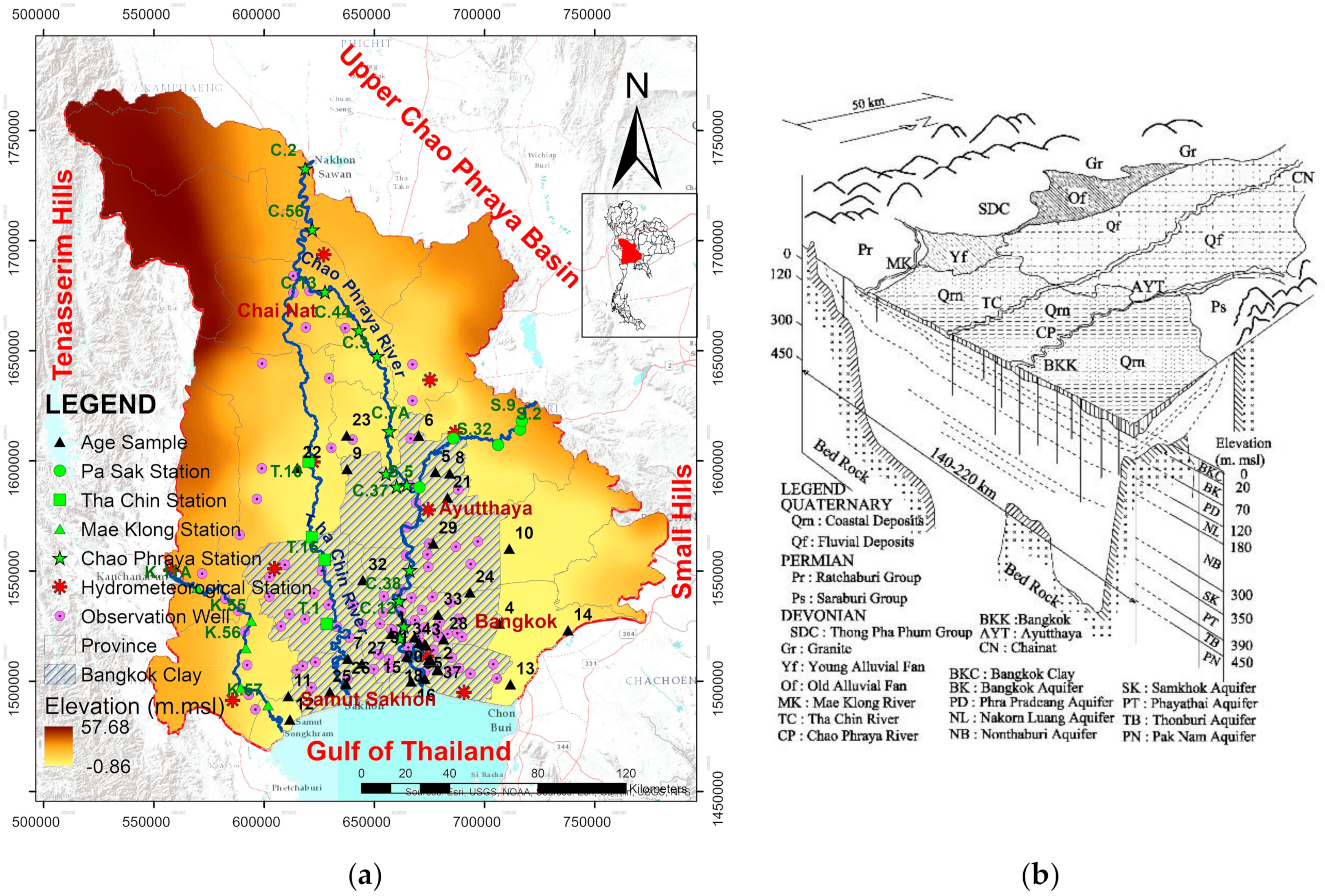
Thailand’s Lower Chao Phraya (LCP) basin is in the central plain. The area is 43,300 km2: the east–west edge is ~230 km and the north–south edge ~300 km (Figure 1a). The west side of the basin is connected to the Tenasserim hills, a long range of hills; groundwater flows through the Upper Chao Phraya basin in the north side; the east side is bounded by a series of small hills and the Gulf of Thailand in the south side. Additionally, this basin has four large rivers, the Chao Phraya, Pa Sak, Tha Chin and Mae Klong Rivers and the surface water flows from north to south.
The hydrogeology was deposited in the Upper Tertiary to Quaternary of the Lower Central Plains of Thailand (Figure 1b). Sands, gravels and clays of the Pliocene-Pleistocene-Holocene were composed and sedimented into eight principal confined aquifers, separated by confining clay lenses [61,62]. These aquifers were covered by Bangkok Clay. The total depth is ~500 m. The primary targets for water well construction were the 2nd (Phra Pradeang; PD), 3rd (Nakorn Luang; NL), 4th (Nonthaburi; NB) aquifers, with depths ranging from 100 to 250 m below the ground surface [63].
The LCP basin was studied here, because it is the largest groundwater supply for the central part of Thailand and covers Bangkok, the capital city. There are many groundwater monitoring stations, which can be used for calibration and verification. However, this region also has a capital city and surrounding urban areas, so there is considerable industrial, domestic and agricultural water consumption. So, groundwater may be in short supply and contaminated. In addition, this region suffered from excessive groundwater extraction, which contributed to land subsidence [63]. Additionally, the basin is located in a tropical climate region and is thus sensitive to climate change [10,11,12,13]. Thus, the LCP basin is important for studying climate change impacts on groundwater resources: the distribution of groundwater age is an indicator, so we investigated the groundwater response and sensitivity.
2.3. Climate
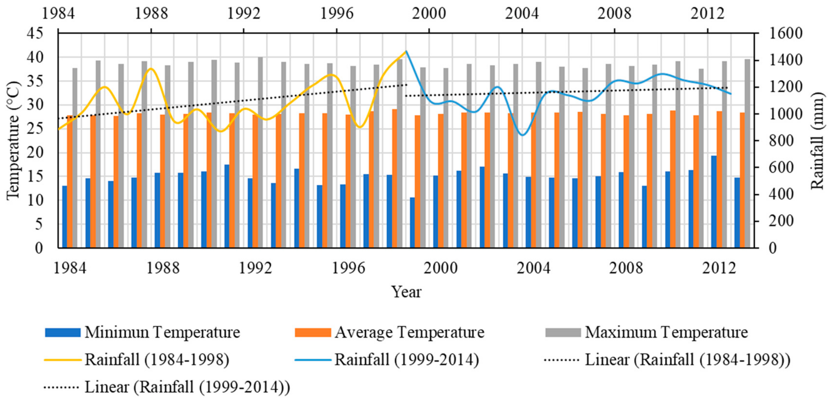
The climate in the study area is tropical: the average daily temperature increased from 27.1 °C in 1984–1998 to 27.4 °C in 1999–2014. December is the coolest month with a daily temperature of ~16.6 °C and ~38.3 °C in April, which was the hottest month during 1984–2014 (Figure 2). The average annual rainfall was calculated using ten hydrometeorological stations between 1984 and 2014 (Figure 1a). Almost 60% of rainfall occurred in the rainy season from May to October. The annual rainfall varied from 1000 to 1675 mm (average = 1155 mm). Climate change led to changes in temperature and precipitation patterns [9,10] and, in the tropical LCP basin [10,11,12,13], the recharge rate changed with the climate, which, in turn, led to groundwater age change.
However, in this research, temperature was omitted, because groundwater aquifer was at a 50–100 m depth, thus change in air temperature did not impact the temperature of groundwater.
2.4. Groundwater Age Collection
Sanford and Buapeng [45] measured isotopic ratios for 18O, 2H, 3H, 13C and 14C, in Thailand, from 1987 to 1996. More than 150 groundwater samples were collected with 1 m well screen lengths, so samples were taken from one aquifer only. About 50 samples were analyzed for 14C, which is the indicator for the groundwater age, because 14C was not contaminated by either 3H or seawater and the regional groundwater is in the 5730-year range for the 14C half-life. Groundwater age from 14C dating was calculated from:
where 5730 is the 14C half-life, A is the 14C concentration (as percent of modern carbon) in the groundwater, and A0 is the fraction of the current total carbon concentration, attributable to carbon in the recharge area.
Table 1 shows the 14C-based ages of groundwater from selected wells in the LCP Basin [45]. The groundwater age was 8500 (PD), 13,000 (NL) and 10,200 (NB) years, with mean ~11,000 years. This showed that groundwater is “young” (>50 years and <12,000 years) or fossil groundwater (>12,000 years), following the labels applied by Bierkens and Wada, Gleeson et al., and Jasechko et al. [50,64,65].
3. Methods
3.1. Model Concept and Boundary Conditions
The model used was described by Tanachaichoksirikun et al. [60] and derived from a database that included hydraulic parameters (hydraulic conductivity and specific storage), groundwater budgets (recharge, pumping and river), topographic data (Digital Elevation Model: DEM and aquifer thickness) and boundary conditions (no-flow boundary and constant head), that was calibrated by matching groundwater hydraulic head, hydraulic gradient and sensitivity of recharge and pumping in 2009–2014. The parameters used were the same as those used for verification in 2007–2008.
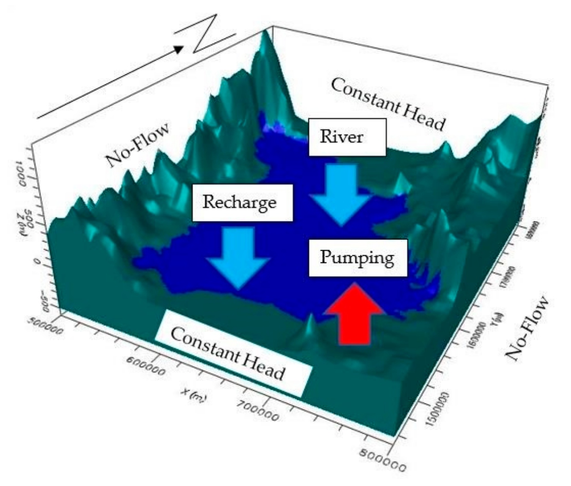
Figure 3 shows a 3D groundwater model of the LCP basin. The groundwater model was separated into nine layers—eight for groundwater aquifers and a topmost layer for Bangkok Clay (BKC). A constant head was assigned in the north side for groundwater flow from the Upper Chao Phraya basin and in the south for the tidal water of the Gulf of Thailand, using the hydraulic head near the edge. River boundaries were applied for four rivers using data from 27 river monitoring stations and calculated following Harbaugh et al. [52]. The recharge boundaries were defined by land use, soil property and rainfall intensity [4,23]. Below the lowest layer, there was a no-flow boundary of impermeable bed rock. The west edge had a no-flow boundary for the Tenasserim hills, and the east had a no-flow boundary defined by small hills. In addition, the major groundwater pumping in PD, NL, NB aquifers—due to their heavy consume groundwater for domestic, industry and agriculture and many available data for calibration and validation—were treated as pumping. For these reasons, this research focused on the groundwater age distribution in these aquifers.
3.2. Hydraulic Parameters
Hydraulic parameter data were derived from our previous study [60]: we considered a hydraulic gradient technique to estimate hydraulic parameters, hydraulic conductivity and anisotropy and concluded that the anisotropy of the LCP basin was 104. In addition, here, we considered the porosity using the observed groundwater age from data of Sanford and Buapeng [45] and followed Meyer et al.’s technique [66]. The groundwater age data were used for verifying porosity of the LCP basin at the sampled points. Backward tracking was applied from the derived age in the observation well to the source, to compare with the model prediction. The groundwater parameters are shown in Table 2.
3.3. Future Climate Scenarios
The Intergovernmental Panel on Climate Change (IPCC) [8] developed a new greenhouse gas model, the Representative Concentration Pathways (RCP), reported in The Fifth Assessment Report (AR5). RCP was developed by using an initial greenhouse gas concentration and predicting the impact on climate change for several greenhouse levels. RCPs used here were based on four scenarios, i.e., RCP2.6, RCP4.5, RCP6.0 and RCP8.5. The numbers, 2.6, 4.5, 6.0 and 8.5, are labels for a set of representative pathways greenhouse gas concentrations defined in the IPCC AR5 report.
We assumed that climate change was reflected in changes in rainfall and that the recharge rate was directly related to rainfall. The projected climate scenario during 2020–2099 was derived from Wattanasetpong et al. [67], based on records for 30 years of Thailand’s LCP monitoring stations and the Royal Netherlands Meteorological Institute (KNMI) Climate Explorer [68]. They considered the six important criteria for climate change—rainfall, temperature, pressure, humidity, evaporation and water discharge to the ocean. Ruangrassamee et al. [69] investigated and showed that the IPSL-CM5A-MR (Institute Pierre Simon Laplace) scenario was optimal for the Chao Phraya water shed, because the climate model was a minimum root-mean-square error and no bias data. Additionally, three Representative Concentration Pathways (RCP) values were selected—2.6, 4.5 and 8.5—as representatives of a range of carbon dioxide concentrations and rainfall rates, where RCP 4.5 represents rainfall close to the present [67]. RCP 6.0 was not considered, because it represents an intermediate scenario between RCP4.5 and RCP8.5.
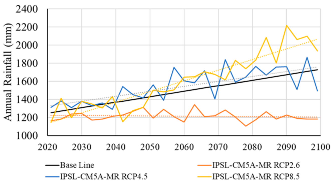
Figure 4 illustrates the predicted future climate from downscaling projected annual rainfall from IPSL-CM5A-MR under the RCP 2.6, 4.5 and 8.5 models, from 2020 to 2099, compared to a baseline trend [67]. The baseline period was based on rainfall from 1984 to 2014 for checking the change in groundwater age distribution with climate change. In the climate scenarios, monthly precipitation was predicted for 2020 to 2099 [67]. We predicted groundwater sustainability in the basin by analyzing movement of groundwater from the groundwater age distribution. Note, future groundwater extraction assumed a pumping rate that was the same as the baseline, because the area showed a very slowly increasing pumping rate.
The annual rainfall trends predicted by the various model are shown in Figure 4. The annual rainfall of the RCP 2.6 model showed a gradually increasing trend, whereas the RCP 8.5 annual rainfall had a significantly increasing trend from 2020 to 2099. However, the RCP 4.5 model showed a more slowly increasing trend than the RCP 8.5 model, in the period 2036–2099. IPSL-CM5A-MR with RCP 8.5 predicted the highest rainfall (↑7.4%), whereas IPSL-CM5A-MR RCP 2.6 predicted the smallest (↓17.4%). Close to the current trends were found in IPSL-CM5A-MR with RCP 4.5 (↑3.1%).
3.4. Predicted Groundwater Age
We focused on change in groundwater age under global climate change. The particles, assumed to be groundwater samples, were randomly assigned to sampling points in the PD, NL and NB aquifers. The predicted groundwater age distributions were simulated, in every climate scenario using the particle backward tracking method, because we had known sample locations and could track backwards from them. However, we analyzed on a regional scale, because groundwater came from several sources, e.g., mixing between young and old groundwater, pumping and recharge, so the particle was used to infer the geographic distribution of groundwater ages.
For model evaluation, the dataset from 2007–2014 was divided into a calibration period (2009–2014) and a validation period (2007–2008). The MODFLOW-2000 model was calibrated from MODFLOW’s parameter estimation and also manual parameter estimation. The model performance can be considered satisfactory if absolute residual mean error ≤ 5 m, NRSE ≤ 10% and R2 > 0.85 [70]. For model prediction, the 2020–2099 data were projected to predict the groundwater age distribution, using initial particles in the calibration model.
4. Results and Discussion
4.1. Calibration and Verification
The calibration and verification by Tanachaichoksirikun et al. [60] for the correlation of simulated and measured hydraulic head is shown in Figure 5. In Figure 5a, the simulated and measured hydraulic heads were compared, in 2009–2014, with an absolute residual mean error of 4.6 m and NRSE = 5.9% and R2 = 0.91.
In the verification model (Figure 5b), the simulated and measured hydraulic heads were compared in 2007–2008. The absolute residual mean error was 2.6 m, with NRSE = 3.8% with R2 = 0.95. So, our errors were less than those of Du et al. [70], often used as a benchmark for numerical simulation of groundwater flow: for any node, the absolute residual mean error should be less than 5 m, with NRSE < 10%.
In addition, here, we calibrated using change in hydraulic gradient to anisotropy as in our previous work [60]. The calibration using only the hydraulic head was not sufficient in a regional scale, because the LCP basin is alluvial. The aquifers are sedimentary units, with high anisotropy. the data showed that the optimal anisotropy was 104, due to the high correlation between hydraulic head and hydraulic gradient (R2 > 0.8). Additionally, this model was analyzed for sensitivity to recharge and pumping and showed that groundwater flow was comparable with the real-world condition.
4.2. Simulated Versus Observed Groundwater Age
Figure 6 shows a close agreement between the observed 14C groundwater ages from Sanford and Buapeng [45] (over 11,000 years) and our simulation (over 10,733 years). The standard deviation was 3300 years, with R2 = 0.81. Thus, this model can be used for predicting groundwater age distribution: R2 > 0.8 and standard deviations in the range of 2000–4000 years [45].
4.3. Predicted Groundwater Age Distribution
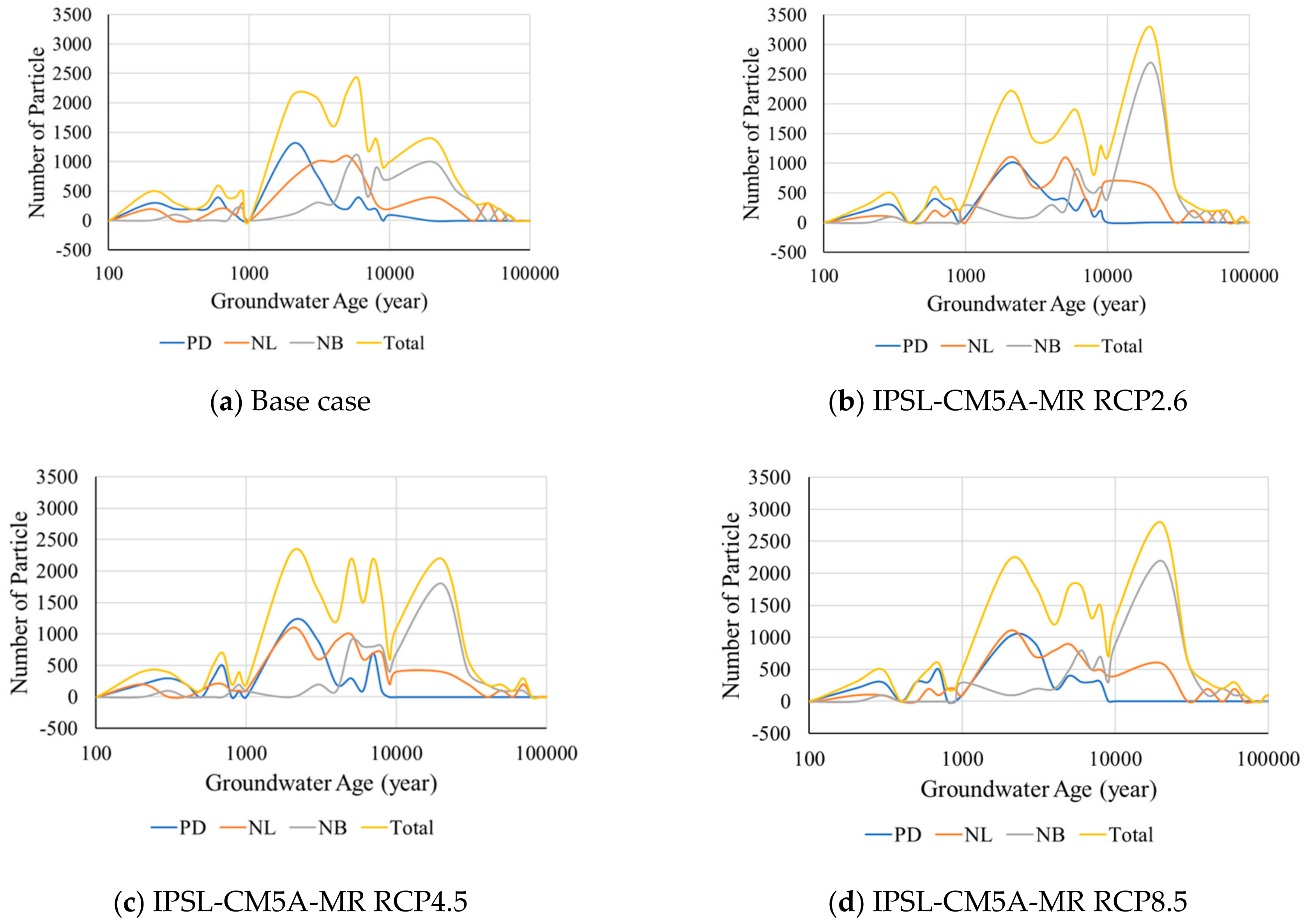
Figure 7 illustrates the groundwater age distribution in the LCP basin, for the base case and IPSL-CM5A-MR with RCP 2.6, 4.5 and 8.5. The groundwater age was shown separately for each aquifer and overall. In general, the younger groundwater was near the recharge and injection zones, where the groundwater age is zero and increased with gradient and depth. The groundwater age in the LCP basin was distributed widely, i.e., ages varied over a wide range; because of the regional basin, some groundwater was resident for a long time, travelled long distances and several sources of water were involved—as discussed in the previous section.
Under the base case (Figure 7a), groundwater age in the PD aquifer covered 100 to 10,000 years, and the mean groundwater age was ~2800 years. The groundwater age in the NL aquifer covered 100–70,000 years, and the mean age was ~8000 years. The NB aquifer distribution covered 1000–100,000 years with a mean age of ~14,500 years. Overall, the average age was ~11,000 years. Thus, the study area was mainly old groundwater. Groundwater flowed slowly, because the basin was a sedimentary aquifer and clay layers between the aquifers hindered groundwater flow from the surface area to the aquifer.
Under RCP2.6 (Figure 7b), groundwater age in the PD aquifer was 100 to 9000 years, with average age = 2988 years (i.e., 188 years longer than the base case). The average age distribution was 67% wider than the base case. Groundwater age in the NL aquifer was 200–80,000 years, with an average of 8986 years (+985 years from the base case). The age distribution was also wider, by 80.1%, compared to the base. Groundwater age in the NB aquifer was 1000–120,000 years. The average age = 18,253 years (+3745 years from the base). The age distribution was 62% wider than the base case. This showed that the lower rainfall contributed to increased groundwater age. The lower rainfall contributed to decreased recharge, low groundwater budget, which, in turn, led to lower hydraulic head and lower velocity. The shallow aquifer was affected by the climate change, due to lower distance and thinner clay layers.
Under RCP4.5 (Figure 7c), groundwater age in the PD aquifer was 100–8000 years with average = 2850 years (+50 years). The distribution was 59% wider. Groundwater age in the NL aquifer ranged from 100 to 70,000 years. The average age was 7967 years (−34 years, i.e., less than the base case). The distribution was wider by 83.2%. In the NB aquifer, groundwater age covered 800–120,000 years with average = 14,911 years (+411 years). The distribution was 59% wider. This showed that the predicted rainfall was close to the base case. The groundwater age was similar to the base case.
Under RCP8.5 (Figure 7d), groundwater age in the PD aquifer covered 100–8000 years with the average = 2746 years (−69 years). The distribution was 80% wider. Groundwater age in the NL aquifer covered 100–60,000 years. The average age = 8914 years (+913 years). The distribution was 89% wider. In the NB aquifer, groundwater age covered 1000–120,000 years, with average = 17,378 years (+2870 years). The distribution was 62% wider. This showed that the higher rainfall led to decreased groundwater age in a shallower aquifer, but in a deeper aquifer, groundwater age was apparently still increasing, but our simulation time extended only to 100 years. The rainfall had not flowed to the NB aquifer, so the groundwater age in NB was increased.
Additionally, the average groundwater age in a shallow aquifer was younger than in a deeper one. The groundwater age distribution in the PD aquifer covered 100–10,000 years, whereas, in the NL and NB aquifers, it extended to 100,000 years.
Although Engdahl and Maxwell [49] suggested that climate change affected groundwater age, our work showed that groundwater age changed only slightly in transient groundwater flow conditions, because the climate change was not accompanied by high rainfall, at that time. In higher recharge scenarios, e.g., IPSL 8.5, the groundwater age distribution shifted slightly, because rainfall increased groundwater velocity and rain generated more surface water. In contrast, in lower recharge scenarios, e.g., IPSL 2.6, the groundwater age shifted significantly, because lower rainfall caused longer residence times and reduced flux (slower velocities).
Overall, changing groundwater age distributions, with differing climate change scenarios, reflected many changes of hydraulic head, recharge and velocity. The change in the age distributions showed the dynamics of the groundwater systems, as fractions of groundwater shifted slightly at various ages, from 10 to 100 years as shown in Figure 7. The age distribution changes indicated changes in location and rate of recharge. Then, groundwater levels, that cause land subsidence, may be unstable. In climate change scenarios, with increased rainfall, making the regional system wetter, the upper aquifer was more completely filled and the excessive groundwater flowed to the surface water system. Groundwater age distributions were unaffected. Change in water budget between surface and groundwater was reduced and caused an increase in older groundwater, although the groundwater ages rarely changed.
4.4. Distribution of Groundwater Age under Climate Change Impact
The projected climate change, under the IPSL-CM5A-MR, was simulated to check for future groundwater age. More recharge, therefore, increasing groundwater levels, led to younger groundwater in shallow aquifers and older water in deeper aquifers. Thus, future groundwater recharge is the most significant feature that controls decrease or increase of age in each aquifer. Increased future groundwater age and the time to recharge was longer than human life spans, which indicated that groundwater in the LCP basin is nonrenewable groundwater. The groundwater recharge affected the groundwater fluctuation, which led to the groundwater problems, e.g., land subsidence and seawater intrusion.
In the shallower aquifer, groundwater ages decreased because, as older groundwater was pumped out of the lower aquifer, it was replaced by younger groundwater from the upper layer. The old groundwater that was pumped out of the aquifer cannot be replaced by recharge, because the effects of old groundwater were replaced by young water in the upper part of the aquifer and mixed with low velocity.
Nonrenewable groundwater will contribute to land subsidence and consequent detrimental effects, e.g., damage to infrastructure and increased flood damage and risk due to lower ground surface level [71]. Soil is an elastic material, so if groundwater is recovered, the soil level will be increased. However, if groundwater level decreased for long periods and contributed to land subsidence for longer times, soil material will creep and become inelastic, so although groundwater level is restored, the land will not return to previous levels.
Since the LCP basin connects to the Gulf of Thailand, pumping groundwater has led to a progressive increase in salinity: decrease in hydraulic head, under the influence of pumping, especially in low recharge scenarios, led to rise of the sea–groundwater interface, leading to more saline groundwater resources. This effect was more obvious in the shallower aquifers, because of the higher sensitivity to hydraulic heads and to higher pumping, induced by lower costs.
The predicted increase in groundwater age from recharge will affect the groundwater level. Therefore, groundwater pumping must be carefully managed, because it may cause land subsidence, seawater intrusion and salinity. Moreover, pumping in nonrenewable groundwater may contribute to groundwater shortage, because rainfall cannot recharge it in human life spans. Here, we showed that the groundwater age distribution, in the deeper layers, i.e., the NL and NB aquifers, will gradually increase in the order of 100 years, indicating that recharge will not fill these aquifers; therefore, pumping in these aquifers must be carefully managed.
5. Conclusions
Variations in precipitation and recharge affect groundwater age distributions on regional scales. We assessed the distributions of groundwater age, under climate change in several scenarios, in Thailand’s Lower Chao Phraya (LCP) basin. The optimal climate scenario, IPSL-CM5A-MR, derived in work by Ruangrassamee et al. and Wattanasetpong et al. [67,69], was used here, and we varied the Representative Concentration Pathway (RCP) models (labeled 2.6, 4.5 and 8.5), from 2020 to 2099. Simulations used MODFLOW-2000 and MODPATH under transient-state conditions. We found that groundwater age slightly decreased in the shallower aquifers, whereas the age increased in the deeper aquifers, under increasing recharge scenarios, because current rainfall did not move water to the deep aquifers. The overall average groundwater age gradually increased, due to groundwater age mixing in both shallow and deep aquifers. However, under decreasing recharge scenarios, groundwater age increased in both shallow and deep aquifers, because reduction of recharge caused groundwater to flow slower and for longer times, so that groundwater became older, which was also reflected in decreased in hydraulic heads.
The fluctuation of groundwater recharge led to change in groundwater age, which was an indicator of the groundwater level, which, in turn, allowed for land subsidence, seawater intrusion and increased salinity. Further, groundwater became short in the area, if groundwater was over pumped, especially in the NL and NB aquifers, where groundwater age increased in both increased and decreased recharge scenarios.
Author Contributions
P.T. established the groundwater flow model and prepared the manuscript. U.S. provided the conceptualization, idea and suggestion and edited the manuscript. All authors have read and agreed to the published version of the manuscript.
Funding
This research was funded by the Thailand Research Fund through the Royal Golden Jubilee Ph.D. Program, Grant No. PHD/189/2556.
Acknowledgments
We give special thanks to the Royal Golden Jubilee Program (Grant No. PHD/0189/2556) from the Thailand Research Fund for financial support and to the Thailand Meteorological Department for the meteorological data, the Thailand Land Development Department for the topographic map and the Thailand Department of Groundwater Resources for the data and additional support.
Conflicts of Interest
The authors declare no conflict of interest.
References
- Tanachaichoksirikun, P.; Seeboonruang, U. Effect of Climate Change on Groundwater Age of Thailand’s Lower Chao Phraya Basin. In Proceedings of the 5th International Conference on Engineering, Applied Sciences and Technology, Luang Prabang, Laos, 2–5 July 2019; p. 639. [Google Scholar]
- Ali, R.; McFarlane, D.; Varma, S.; Dawes, W.; Emelyanova, I.; Hodgson, G.; Charles, S. Potential climate change impacts on groundwater resources of south-western Australiarn Australia. J. Hydrol. 2012, 475, 456–472. [Google Scholar] [CrossRef]
- Singh, R.D.; Kumar, C.P. Impact of Climate Change on Groundwater Resources. In Proceedings of the 2nd National Ground Water Congress, Uttarakhand, India, 22 March 2010; Volume 247667, pp. 196–221. [Google Scholar]
- Pholkern, K.; Saraphirom, P.; Srisuk, K. Potential impact of climate change on groundwater resources in the Central Huai Luang Basin, Northeast Thailand. Sci. Total Environ. 2018, 633, 1518–1535. [Google Scholar] [CrossRef] [PubMed]
- Foster, S.; Loucks, D.P. Non-Renewable Groundwater Resources-a Guide to Socially-Sustainable Management for Water-Policy Makers; IHP Series on Groundwater Unesco: Paris, France, 2006. [Google Scholar]
- Lachaal, F.; Bédir, M.; Tarhouni, J.; Leduc, C. Hydrodynamic and hydrochemical changes affecting groundwater in a semi-arid region: The deep Miocene aquifers of the Tunisian Sahel (central east Tunisia). IAHS-AISH Publ. 2010, 340, 374–381. [Google Scholar]
- Mackay, A. Climate Change 2007: Impacts, Adaptation and Vulnerability. Contribution of Working Group II to the Fourth Assessment Report of the Intergovernmental Panel on Climate Change. J. Environ. Qual. 2008, 37, 2407. [Google Scholar] [CrossRef]
- IPCC. Climate Change 2014. Synthesis Report. Versión Inglés; IPCC: Geneva, Switzerland, 2014; ISBN 9789291691432. [Google Scholar]
- Sieler, K.P.; Gu, W.Z.; Stichler, W. Transient response of groundwater systems to climate changes. Geol. Soc. Spec. Publ. 2008, 288, 111–119. [Google Scholar] [CrossRef]
- Green, T.R.; Taniguchi, M.; Kooi, H.; Gurdak, J.J.; Allen, D.M.; Hiscock, K.M.; Treidel, H.; Aureli, A. Beneath the surface of global change: Impacts of climate change on groundwater. J. Hydrol. 2011, 405, 532–560. [Google Scholar] [CrossRef] [Green Version]
- Chris, M.H.; Harm, D.; Diana, M.A.; Dirk, K. Groundwater Recharge and Storage Variability in Southern Mali. In Climate Change Effects on Groundwater Resources: A Global Synthesis of Findings and Recommendations; CRC Press/Balkema, Taylor and Francis Group: London, UK, 2012; pp. 33–48. [Google Scholar]
- Taylor, R.; Callist, T. The impacts of climate change and rapid development on weathered crystalline rock aquifer systems in the humid tropics of sub-Saharan Africa: Evidence from south-western Uganda. In Climate Change Effects on Groundwater Resources: A Global Synthesis of Findings and Recommendations; Treidel, H., Martin-Bordes, J.L., Gurdak, J.J., Eds.; CRC Press/Balkema, Taylor and Francis Group: London, UK, 2012; pp. 17–32. [Google Scholar]
- White, I.; Tony, F. Reducing Groundwater Vulnerability in Carbonate Island Countries in the Pacific. In Climate Change Effects on Groundwater Resources: A Global Synthesis of Findings and Recommendations; CRC Press/Balkema, Taylor and Francis Group: London, UK, 2012; pp. 75–110. [Google Scholar]
- Tremblay, L.; Larocque, M.; Anctil, F.; Rivard, C. Teleconnections and interannual variability in Canadian groundwater levels. J. Hydrol. 2011, 410, 178–188. [Google Scholar] [CrossRef]
- Goderniaux, P.; Brouyère, S.; Wildemeersch, S.; Therrien, R.; Dassargues, A. Uncertainty of climate change impact on groundwater reserves-Application to a chalk aquifer. J. Hydrol. 2015, 528, 108–121. [Google Scholar] [CrossRef] [Green Version]
- Jackson, C.R.; Meister, R.; Prudhomme, C. Modelling the effects of climate change and its uncertainty on UK Chalk groundwater resources from an ensemble of global climate model projections. J. Hydrol. 2011, 399, 12–28. [Google Scholar] [CrossRef]
- Intergovernmental Panel on Climate Change. IPCC Special Report Enissions Scenarios: Summary for Policymakers; Cambridge University Press: Cambridge, UK, 2000. [Google Scholar]
- Döll, P. Vulnerability to the impact of climate change on renewable groundwater resources: A global-scale assessment. Environ. Res. Lett. 2009, 4, 1–12. [Google Scholar] [CrossRef]
- Emelyanova, I.; Ali, R.; Dawes, W.; Varma, S.; Hodgson, G.; McFarlane, D. Evaluating the cumulative rainfall deviation approach for projecting groundwater levels under future climate. J. Water Clim. Chang. 2013, 4, 317–337. [Google Scholar] [CrossRef]
- Shrestha, S.; Semkuyu, D.J.; Pandey, V.P. Assessment of groundwater vulnerability and risk to pollution in Kathmandu Valley, Nepal. Sci. Total Environ. 2016, 556, 23–35. [Google Scholar] [CrossRef] [PubMed]
- Malekinezhad, H.; Banadkooki, F.B. Modeling impacts of climate change and human activities on groundwater resources using modflow. J. Water Clim. Chang. 2018, 9, 156–177. [Google Scholar] [CrossRef]
- Taylor, R.G.; Scanlon, B.; Döll, P.; Rodell, M.; Van Beek, R.; Wada, Y.; Longuevergne, L.; Leblanc, M.; Famiglietti, J.S.; Edmunds, M.; et al. Ground water and climate change. Nat. Clim. Chang. 2013, 3, 322–329. [Google Scholar] [CrossRef] [Green Version]
- Saraphirom, P.; Wirojanagud, W.; Srisuk, K. Potential Impact of Climate Change on Area Affected by Waterlogging and Saline Groundwater and Ecohydrology Management in Northeast Thailand. Environ. Asia 2013, 6, 19–28. [Google Scholar]
- Lee, L.J.E.; Lawrence, D.S.L.; Price, M. Analysis of water-level response to rainfall and implications for recharge pathways in the Chalk aquifer, SE England. J. Hydrol. 2006, 330, 604–620. [Google Scholar] [CrossRef]
- Cook, P.G.; Herczeg, A.L. Environmental Tracers in Subsurface Hydrology; Kluwer Academic Publishers: Boston, MA, USA, 2000. [Google Scholar]
- Kazemi, G.A.; Lehr, J.H.; Pierre, P. Groundwater Age; John Wiley & Sons: Hoboken, NJ, USA, 2006. [Google Scholar]
- Sanford, W.E.; Plummer, L.N.; Mcada, D.P.; Bexfield, L.M.; Anderholm, S.K. Hydrochemical tracers in the middle Rio Grande Basin, USA: 2. Calibration of a groundwater-flow model. Hydrogeol. J. 2004, 12, 389–407. [Google Scholar] [CrossRef]
- Manning, A.H.; Solomon, D.K. An integrated environmental tracer approach to characterizing groundwater circulation in a mountain block. Water Resour. Res. 2005, 41, 1–18. [Google Scholar] [CrossRef] [Green Version]
- Bethke, C.M.; Johnson, T.M. Groundwater age and groundwater age dating. Annu. Rev. Earth Planet. Sci. 2008, 36, 121–152. [Google Scholar] [CrossRef] [Green Version]
- Molson, J.W.; Frind, E.O. On the use of mean groundwater age, life expectancy and capture probability for defining aquifer vulnerability and time-of-travel zones for source water protection. J. Contam. Hydrol. 2012, 127, 76–87. [Google Scholar] [CrossRef]
- Zhu, Y.; Shi, L.; Wu, J.; Ye, M.; Cui, L.; Yang, J. Regional Quasi-three-dimensional unsaturated-saturated water flow model based on a vertical-horizontal splitting concept. Water 2016, 8, 195. [Google Scholar] [CrossRef] [Green Version]
- Sonnenborg, T.O.; Scharling, P.B.; Hinsby, K.; Rasmussen, E.S.; Engesgaard, P. Aquifer vulnerability assessment based on sequence stratigraphic and 39Ar transport modeling. Ground Water 2016, 54, 214–230. [Google Scholar] [CrossRef] [PubMed]
- Troldborg, L.; Jensen, K.H.; Engesgaard, P.; Refsgaard, J.C.; Hinsby, K. Using Environmental Tracers in Modeling Flow in a Complex Shallow Aquifer System. J. Hydrol. Eng. 2008, 13, 1037–1048. [Google Scholar] [CrossRef]
- Eberts, S.M.; Böhlke, J.K.; Kauffman, L.J.; Jurgens, B.C. Comparison of particle-tracking and lumped-parameter age-distribution models for evaluating vulnerability of production wells to contamination. Hydrogeol. J. 2012, 20, 263–282. [Google Scholar] [CrossRef]
- Torgersen, T.; Purtschert, R.; Phillips, F.M.; Plummer, L.N.; Sanford, W.E.; Suckow, A. Defining Groundwater Age. In Isotope Methods Dating Old Groundwater; International Atomic Energy Agency: Vienna, Austra, 2013; pp. 21–32. [Google Scholar]
- Goode, D.J. Direct simulation of groundwater age. Water Resour. Res. 1996, 32, 289–296. [Google Scholar] [CrossRef]
- Ginn, T.R. On the distribution of multicomponent mixtures over generalized exposure time in subsurface flow and reactive transport: Foundations, and formulations for groundwater age, chemical heterogeneity, and biodegradation. Water Resour. Res. 1999, 35, 1395–1407. [Google Scholar] [CrossRef]
- Varni, M.; Carrera, J. Simulation of groundwater age distributions. Water Resour. Res. 1998, 34, 3271–3281. [Google Scholar] [CrossRef]
- Woolfenden, L.R.; Ginn, T.R. Modeled ground water age distributions. Ground Water 2009, 47, 547–557. [Google Scholar] [CrossRef]
- Suckow, A. The age of groundwater-Definitions, models and why we do not need this term. Appl. Geochem. 2014, 50, 222–230. [Google Scholar] [CrossRef]
- Sanford, W. Calibration of models using groundwater age. Hydrogeol. J. 2011, 19, 13–16. [Google Scholar] [CrossRef]
- Michael, H.A.; Voss, C.I. Estimation of regional-scale groundwater flow properties in the Bengal Basin of India and Bangladesh. Hydrogeol. J. 2009, 17, 1329–1346. [Google Scholar] [CrossRef]
- Portniaguine, O.; Solomon, D.K. Parameter estimation using groundwater age and head data, Cape Cod, Massachusetts. Water Resour. Res. 1998, 34, 637–645. [Google Scholar] [CrossRef]
- Engdahl, N.B.; Ginn, T.R.; Fogg, G.E. Using groundwater age distributions to estimate the effective parameters of Fickian and non-Fickian models of solute transport. Adv. Water Resour. 2013, 54, 11–21. [Google Scholar] [CrossRef] [Green Version]
- Sanford, W.E.; Buapeng, S. Assessment of a ground water flow model of the Bangkok Basin, Thailand, using carbon-14-based ages and paleohydrology. Hydrogeol. J. 1996, 4, 26–40. [Google Scholar] [CrossRef]
- Ginn, T.R.; Haeri, H.; Massoudieh, A.; Foglia, L. Notes on groundwater age in forward and inverse modeling. Transp. Porous Media 2009, 79, 117–134. [Google Scholar] [CrossRef] [Green Version]
- Weissmann, G.S.; Zhang, Y.; LaBolle, E.M.; Fogg, G.E. Dispersion of groundwater age in an alluvial aquifer system. Water Resour. Res. 2002, 38, 16-1–16-13. [Google Scholar] [CrossRef]
- Cornaton, F.; Perrochet, P. Groundwater age, life expectancy and transit time distributions in advective-dispersive systems: 1. Generalized reservoir theory. Adv. Water Resour. 2006, 29, 1267–1291. [Google Scholar] [CrossRef] [Green Version]
- Engdahl, N.B.; Maxwell, R.M. Quantifying changes in age distributions and the hydrologic balance of a high-mountain watershed from climate induced variations in recharge. J. Hydrol. 2015, 522, 152–162. [Google Scholar] [CrossRef]
- Bierkens, M.F.P.; Wada, Y. Non-renewable groundwater use and groundwater depletion: A review. Environ. Res. Lett. 2019, 14. [Google Scholar] [CrossRef]
- Jyrkama, M.I.; Sykes, J.F. The impact of climate change on spatially varying groundwater recharge in the grand river watershed (Ontario). J. Hydrol. 2007, 338, 237–250. [Google Scholar] [CrossRef]
- Harbaugh, A.W.; Banta, E.R.; Hill, M.C.; McDonald, M.G. MODFLOW-2000, The, U.S. Geological Survey Modular Ground-Water Model-User Guide to Modularization Concepts and the Ground-Water Flow Process; Geological Survey: Reston, VA, USA, 2000.
- Bear, J. Dynamics of Fluids in Porous Media; Elsevier: New York, NY, USA, 1972. [Google Scholar]
- Pollock, D. User Guide for MODPATH Version 6: A Particle Tracking Model for MODFLOW: Tech. Methods 6–A41; Geological Survey: Reston, VA, USA, 2012; Volume 58. [Google Scholar]
- Fioreze, M.; Mancuso, M.A. MODFLOW and MODPATH for hydrodynamic simulation of porous media in horizontal subsurface flow constructed wetlands: A tool for design criteria. Ecol. Eng. 2019, 130, 45–52. [Google Scholar] [CrossRef]
- Wolfgang-Albert, F.; Michl, C. Using MODFLOW/MODPATH combined with GIS analysis for groundwater modelling in the alluvial aquifer of the River Sieg, Germany. IAHS Publ. 1995, 227, 117–123. [Google Scholar]
- Mondal, N.C.; Singh, V.S. Mass transport modeling of an industrial belt using visual MODFLOW and MODPATH: A case study. J. Geog. 2009, 2, 1–19. [Google Scholar]
- Abrams, D. Correcting Transit Time Distributions in Coarse MODFLOW-MODPATH Models. Ground Water 2013, 51, 474–478. [Google Scholar] [CrossRef] [PubMed]
- Arlai, P.; Koch, M.; Kuntanakulwong, S. Statistical and stochastic approaches to assess reasonable calibrated parameters in a complex multi-aquifer system. In Proceedings of the CMWR XVI-Computational Methods in Water Resources, Copenhagen, Denmark, 19–22 June 2006; pp. 1–8. [Google Scholar]
- Tanachaichoksirikun, P.; Seeboonruang, U.; Fogg, G.E. Improving Groundwater Model in Regional Sedimentary Basin Using Hydraulic Gradients. KSCE J. Civ. Eng. 2020, 24, 1655–1669. [Google Scholar] [CrossRef]
- Piancharoen, C. Groundwater and land subsidence in Bangkok, Thailand. IAHS Publ. 1977, 355–364. [Google Scholar]
- Piancharoen, C.; Chuamthaisong, C. Groundwater of Bangkok metropolis, Thailand. IAH Mem. 1978, 11, 510–528. [Google Scholar]
- Phien-wej, N.; Giao, P.H.; Nutalaya, P. Land subsidence in Bangkok, Thailand. Eng. Geol. 2006, 82, 187–201. [Google Scholar] [CrossRef]
- Gleeson, T.; Befus, K.M.; Jasechko, S.; Luijendijk, E.; Cardenas, M.B. The global volume and distribution of modern groundwater. Nat. Geosci. 2016, 9, 161–167. [Google Scholar] [CrossRef]
- Jasechko, S.; Perrone, D.; Befus, K.M.; Bayani Cardenas, M.; Ferguson, G.; Gleeson, T.; Luijendijk, E.; McDonnell, J.J.; Taylor, R.G.; Wada, Y.; et al. Global aquifers dominated by fossil groundwaters but wells vulnerable to modern contamination. Nat. Geosci. 2017, 10, 425–429. [Google Scholar] [CrossRef] [Green Version]
- Meyer, R.; Engesgaard, P.; Hinsby, K.; Piotrowski, J.; Sonnenborg, T. Estimation of effective porosity in large-scale groundwater models by combining particle tracking, auto-calibration and 14C dating. Hydrol. Earth Syst. Sci. 2018, 22, 4843–4865. [Google Scholar] [CrossRef] [Green Version]
- Wattanasetpong, J.; Charoenvaravut, P.; Laosinwattana, W. Downscaling Climate Models in Thailand by Artificial Neural Network Method; Thesis of Civil Engineering; King Mongkut’s Institute of Technology Ladkrabang: Bangkok, Thailand, 2015. [Google Scholar]
- World Meteorological Organization. World Climate Explorer. Available online: https://climexp.knmi.nl/start.cgi (accessed on 15 September 2015).
- Ruangrassamee, P.; Khamkong, A.; Chuenchum, P. Assessment of precipitation simulations from CMIP5 climate models in Thailand. In Proceedings of the 3rd EIT International Conference on Water Resources Engineering (ICWRE3), Bangkok, Thailand, 5–7 August 2015. [Google Scholar]
- Du, X.; Lu, X.; Hou, J.; Ye, X. Improving the reliability of numerical groundwater modeling in a data-sparse region. Water 2018, 10, 289. [Google Scholar] [CrossRef] [Green Version]
- Sato, C.; Haga, M.; Nishino, J. Land subsidence and groundwater management in Tokyo. Int. Rev. Environ. Strateg. 2006, 6, 403–424. [Google Scholar]
Figure 1.
Thailand’s Lower Chao Phraya Basin location, elevation and stratigraphy: (a) Location and elevation adapted from Tanachaichoksirikun et al. [60], (b) Stratigraphy adapted from Phien-wej et al. [63].

Figure 2.
Rainfall and temperature in 1984–2014.

Figure 3.
3D groundwater model [60].
Figure 3.
3D groundwater model [60].

Figure 4.
Predicted future climate [67].
Figure 4.
Predicted future climate [67].

Figure 5.
Calculated vs. observed heads, (a) Calibration measurements, (b) Verification measurements.
Figure 5.
Calculated vs. observed heads, (a) Calibration measurements, (b) Verification measurements.

Figure 6.
Simulated vs. observed groundwater age.

Figure 7.
Groundwater age distribution in the LCP basin, (a) Base case, (b) IPSL-CM5A-MR RCP2.6, (c) IPSL-CM5A-MR RCP4.5, (d) IPSL-CM5A-MR RCP8.5.
Figure 7.
Groundwater age distribution in the LCP basin, (a) Base case, (b) IPSL-CM5A-MR RCP2.6, (c) IPSL-CM5A-MR RCP4.5, (d) IPSL-CM5A-MR RCP8.5.


Table 1.
14C-based ages of groundwater from selected wells in the Lower Chao Phraya (LCP) Basin [45].
Table 1.
14C-based ages of groundwater from selected wells in the Lower Chao Phraya (LCP) Basin [45].
| Well No. | Model Layer No. | Aquifers Name | Observed Groundwater Age (Years) |
|---|---|---|---|
| 1 | 3 | PD | 7100 |
| 2 | 9100 | ||
| 3 | 7300 | ||
| 4 | 18,100 | ||
| 5 | 5300 | ||
| 6 | 6900 | ||
| 7 | 9500 | ||
| 8 | 9800 | ||
| 9 | 5200 | ||
| 10 | 8300 | ||
| 11 | 18,300 | ||
| 12 | 6800 | ||
| 13 | 10,000 | ||
| 14 | 7700 | ||
| 15 | 8500 | ||
| 16 | 5700 | ||
| 17 | 2300 | ||
| 18 | 4 | NL | 8100 |
| 19 | 7400 | ||
| 20 | 8900 | ||
| 21 | 18,900 | ||
| 22 | 18,100 | ||
| 23 | 5500 | ||
| 24 | 20,900 | ||
| 25 | 19,400 | ||
| 26 | 19,900 | ||
| 27 | 12,500 | ||
| 28 | 8600 | ||
| 29 | 8400 | ||
| 30 | 5 | NB | 6300 |
| 31 | 9000 | ||
| 32 | 8500 | ||
| 33 | 18,200 | ||
| 34 | 1600 | ||
| 35 | 13,800 | ||
| 36 | 9100 | ||
| 37 | 154,000 |
Table 2.
Groundwater parameter in the LCP basin.
| Aquifers | Porosity | Kh (m/s) | Kv (m/s) | Ss (m−1) |
|---|---|---|---|---|
| Bangkok Clay and Unconfined | 0.03 | 1 × 10⁻⁸–1 × 10⁻⁹ | 1 × 10⁻⁸–1 × 10⁻⁹ | 0.03–0.35 (Sy) |
| Bangkok | 0.2–0.3 | 5 ×10⁻⁵–6 × 10⁻⁶ | 5 × 10⁻⁹–6 × 10⁻¹⁰ | 1.10 × 10⁻⁵–4.80 × 10⁻⁵ |
| Phra Pradeang | 0.25–0.35 | 2 × 10⁻⁵–7 × 10⁻⁶ | 2 × 10⁻⁹–7 × 10⁻¹⁰ | 3.35 × 10⁻⁵–4.50 × 10⁻⁶ |
| Nakorn Luang | 0.2–0.35 | 1 × 10⁻⁴–6 × 10⁻⁶ | 1 × 10⁻⁸–6 × 10⁻¹⁰ | 3.85 × 10⁻⁵–9.50 × 10⁻⁶ |
| Nonthaburi | 0.3–0.35 | 2 × 10⁻⁴–7 × 10⁻⁶ | 2 × 10⁻⁸–7 × 10⁻¹⁰ | 3.95 × 10⁻⁵–9.50 × 10⁻⁶ |
Publisher’s Note: MDPI stays neutral with regard to jurisdictional claims in published maps and institutional affiliations. |
© 2020 by the authors. Licensee MDPI, Basel, Switzerland. This article is an open access article distributed under the terms and conditions of the Creative Commons Attribution (CC BY) license (http://creativecommons.org/licenses/by/4.0/).
Share and Cite
MDPI and ACS Style
Tanachaichoksirikun, P.; Seeboonruang, U. Distributions of Groundwater Age under Climate Change of Thailand’s Lower Chao Phraya Basin. Water 2020, 12, 3474. https://doi.org/10.3390/w12123474
AMA Style
Tanachaichoksirikun P, Seeboonruang U. Distributions of Groundwater Age under Climate Change of Thailand’s Lower Chao Phraya Basin. Water. 2020; 12(12):3474. https://doi.org/10.3390/w12123474
Chicago/Turabian StyleTanachaichoksirikun, Pinit, and Uma Seeboonruang. 2020. "Distributions of Groundwater Age under Climate Change of Thailand’s Lower Chao Phraya Basin" Water 12, no. 12: 3474. https://doi.org/10.3390/w12123474
Note that from the first issue of 2016, this journal uses article numbers instead of page numbers. See further details here.