Comparing Q-Tree with Nested Grids for Simulating Managed River Recharge of Groundwater


1
The Institute of Hydrogeology and Environmental Geology, Chinese Academy of Geological Sciences, Shijiazhuang 050061, Hebei, China
2
Key Laboratory of Groundwater Contamination and Remediation of Hebei Province and China Geological Survey, Shijiazhuang 050061, Hebei, China
3
College of Water Resources and Environment, Hebei GEO University, Shijiazhuang 050031, Hebei, China
*
Author to whom correspondence should be addressed.
Water 2020, 12(12), 3516; https://doi.org/10.3390/w12123516
Submission received: 21 October 2020
/
Revised: 6 December 2020
/
Accepted: 12 December 2020
/
Published: 14 December 2020
(This article belongs to the Special Issue Applied Groundwater Modelling for Water Resources Management and Protection)
Abstract
:The use of rivers to recharge groundwater is a key water resource management method. High-precision simulations of the groundwater level near rivers can be used to accurately assess the recharge effect. In this study, we used two unstructured grid refinement methods, namely, the quadtree (Q-tree) and nested grid refinement techniques, to simulate groundwater movement under river recharge. We comparatively analyzed the two refinement methods by considering the simulated groundwater level changes before and after the recharge at different distances from the river and by analyzing the groundwater flow and model computation efficiency. Compared to the unrefined model, the two unstructured grid refinement models significantly improve the simulation precision and more accurately describe groundwater level changes from river recharge. The unstructured grid refinement models have higher calculation efficiencies than the base model (the global refinement model) without compromising the simulation precision too much. The Q-tree model has a higher simulation precision and a lower computation time than the nested grid model. In summary, the Q-tree grid refinement method increases the computation efficiency while guaranteeing simulation precision at a certain extent. We therefore recommended the use of this grid refinement method in simulating river recharge to the aquifers.
1. Introduction
Several countries have carried out aquifer recharge projects, including well infiltration, river recharge, and the refilling of gravel pits [1,2,3,4], to relieve groundwater level decreases and water resource shortages from groundwater overexploitation. The Ministry of Water Resources of the People’s Republic of China started a new managed aquifer recharge projects using river and lake in 2019. During this year, 2.21 × 10⁹ m3 water was replenished to rivers and lakes in the Beijing-Tianjin-Hebei region by the south-to-north water diversion, as well as water diversion from the Yellow and Luan Rivers [5]. Thus, managed aquifer recharge by river has become a highly active field in the North China Plain.
Groundwater modeling is an effective method for studying groundwater flow and simulating aquifer recharge processes. Many scholars have used numerical simulations to investigate the process, effect, and optimization of managed aquifer recharge [6,7,8,9,10]. The grids in regional groundwater models are typically quite large [11]. These models often have difficulty in precisely simulating local groundwater level changes near rivers with significant groundwater level change. In these cases, the local grid refinement of concerned regions is required. However, there has been little consideration of precision in modeling river recharge to groundwater, which proceeds by linear infiltration. In contrast to areal infiltration, the grid generation method used to model linear infiltration near rivers directly affects the simulation results and in turn the assessment of the recharge.
The MODFLOW program is a prevailing program for simulating groundwater movement. Its derivative MODFLOW-USG (Unstructured Grid) generates grids based on the control-volume finite-difference (CVFD) method [12]. Compared with the traditional MODFLOW program, MODFLOW-USG can locally refine grids in some regions (e.g., rivers and mining wells), making the grid generation method more flexible. Krčmář and Sracek used MODFLOW-USG to simulate the Gbely mine region, whereby the geological inhomogeneity in this region related to open pits and tectonic fractures was precisely defined [13]. Shokri et al. also adopted unstructured grids to numerically simulate an unconfined aquifer with a large groundwater hydraulic gradient [14].
MODFLOW-USG have been imbedded into GMS (Groundwater Modeling System), which is an advanced 3D simulation software for groundwater flow and transport modeling [15]. It has three unstructured grid refinement methods, including the quadtree (Q-tree), the nested grid, and Voronoi methods. It is difficult to precisely compare the sizes of the irregular polygonal grids generated by the Voronoi method with the regularly shaped grids generated by the other two methods. Thus, in this study, we only compare the Q-tree and nested grid refinement techniques. We compare simulation results based on two sets of homogeneously structured grids to analyze the pros and cons of using the two unstructured rectangular refinement methods in a linear recharge simulation model. Accordingly, we provide a reference for choosing optimized grid generation methods to simulate managed aquifer recharge processes by rivers.
2. Two Unstructured Grid Refinement Methods
2.1. Q-Tree
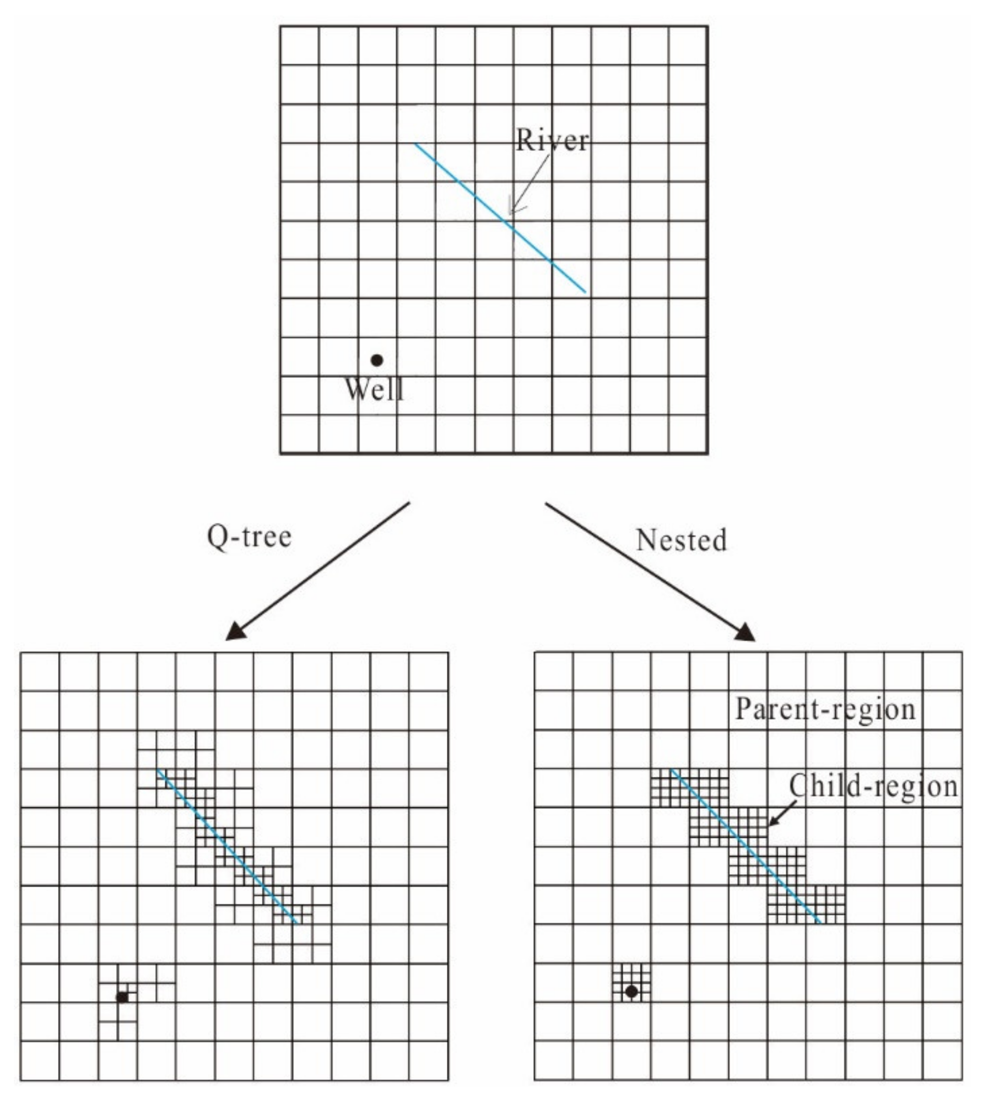
The Q-tree grid generation method was first applied to study image division in computing [16]. First, an image is modeled as a rectangular unit. If the unit contains polygons with different characteristics, the unit is divided into four equally sized secondary units (Figure 1). This step-by-step 1-to-4 method continues until the highest predefined resolution is reached. Then, The Q-tree grid generation technique was further developed and applied to a wide range of fields. Yeery and Shephard used this Q-tree spatial division method to generated grids [17]. In 2001, Rogers et al. from Oxford University first applied Q-tree grids to solve two-dimensional equations [18]. Liu et al. used Q-tree grids to establish a Godunov-type 2D water flow mathematical model and experimentally demonstrated that Q-tree grids are more effective and accurate for modeling regions with complex flows than conventional structured grids [19]. In 2020, Božović et al. used the Q-tree method to generate regions with refined grids, thereby identifying significant groundwater hydraulic gradients and accurately characterizing the movement of groundwater [20].
2.2. Nested Grids
The nested grid method is a local grid refinement technique developed by Mehl and Hill [21]. Using this method, a model is divided into a parent model (an unrefined region) and a child model (a refined region) (Figure 1). The child model homogeneously refines one or more grids in the parent model. The two independent parent and child models are coupled through a series of iterative steps ofgroundwater head and flux through an interface. Nested grid refinement is thus achieved. Using this method, Khan et al. developed a model to illustrate how interactions between aquifer heterogeneity and groundwater exploitation jeopardize groundwater resources regionally [22]. Forghani and Peralta prepared a refined model to evaluate performance of ASR systems in freshwater aquifers [23].
3. A Simplified Model
Our model is a simplified case study generalized from the alluvial fan of the Juma River, which is one of the aquifers receiving managed river recharge. The Juma River is located at the northwest of the North China Plain with semiarid climate condition. The coordinate is 115°41′54″ E-115°58′50″ E, 39°17′43″ N-39°34′50″ N. The altitude varies from 25 m to 52 m. Due to many dam constructions upstream, the runoff had decreased to extremely low level. Most of land is used as farmland and village. To objectively represent the actual situation, we maintained the similar hydrogeological structure, parameters, and boundary conditions (except for the modeling range) for the case study model as the original model during the simplification.
3.1. Model Setup
The model area is at a 10 km × 10 km aquifer with groundwater flowing from west to east (Figure 2). To simplify the hydrogeological conditions of the study area, we generalized the aquifer to an inhomogeneous, anisotropic aquifer system consisting of phreatic and confined water. The model was divided into three layers with thicknesses of 50 m, 100 m, and 100 m with corresponding horizontal permeability coefficients of 50 m/d, 20 m/d, and 7 m/d and vertical permeability coefficients of 0.08 m/d, 0.04 m/d, and 0.02 m/d. The specific yield of the first layer was set to 0.08, and the storativity of both the second and third layers was set to 0.0001.
According to groundwater flow direction, there is water exchange between the east/west boundaries and the aquifer. We defined the boundary on the west side as the flow boundary (Neumann boundary), and the east side as the given head boundary. The other boundaries were defined as no flow. When analyzing the effect of boundary type on the simulation, the west boundary was changed to Dirichlet or general boundary. When it was set as Dirichlet boundary, a fixed value of head at the boundary grid was given in the model. When it was set as Neumann boundary, the fixed flux was given at the boundary grid in the model. When it was set as general boundary, the fixed head was given at a certain distance to the boundary.
The main recharge of aquifer include precipitation, irrigation infiltration, river recharge, etc. Because the local land use type is farmland, a large amount of water is used for irrigation, which would infiltrate into the phreatic aquifer. The intensity of areal recharge from precipitation and irrigation was set to 0.002 m/d.
Water mainly leaves the aquifer as a result of human exploitation and lateral flow. A total number of 9 pumping wells were given in the model (6 wells in the first layer, 2 in the second layer, and 1 in the third layer, as illustrated in (Figure 2). The groundwater exploitation was set to 4000 m3/d for each well.
The simulation period was set to 1 year, each half month was set to a stress period, and each day corresponded to a time step. The volume of groundwater recharged from the river infiltration was assigned to grids in the first layer in the form of wells, the average volume of groundwater recharged from the river was set to 1.5 × 10⁵ m3/d, and the recharge period was set to 1 year.
3.2. Four Grid Generation Schemes
We adopted four different grid generation schemes for comparison.
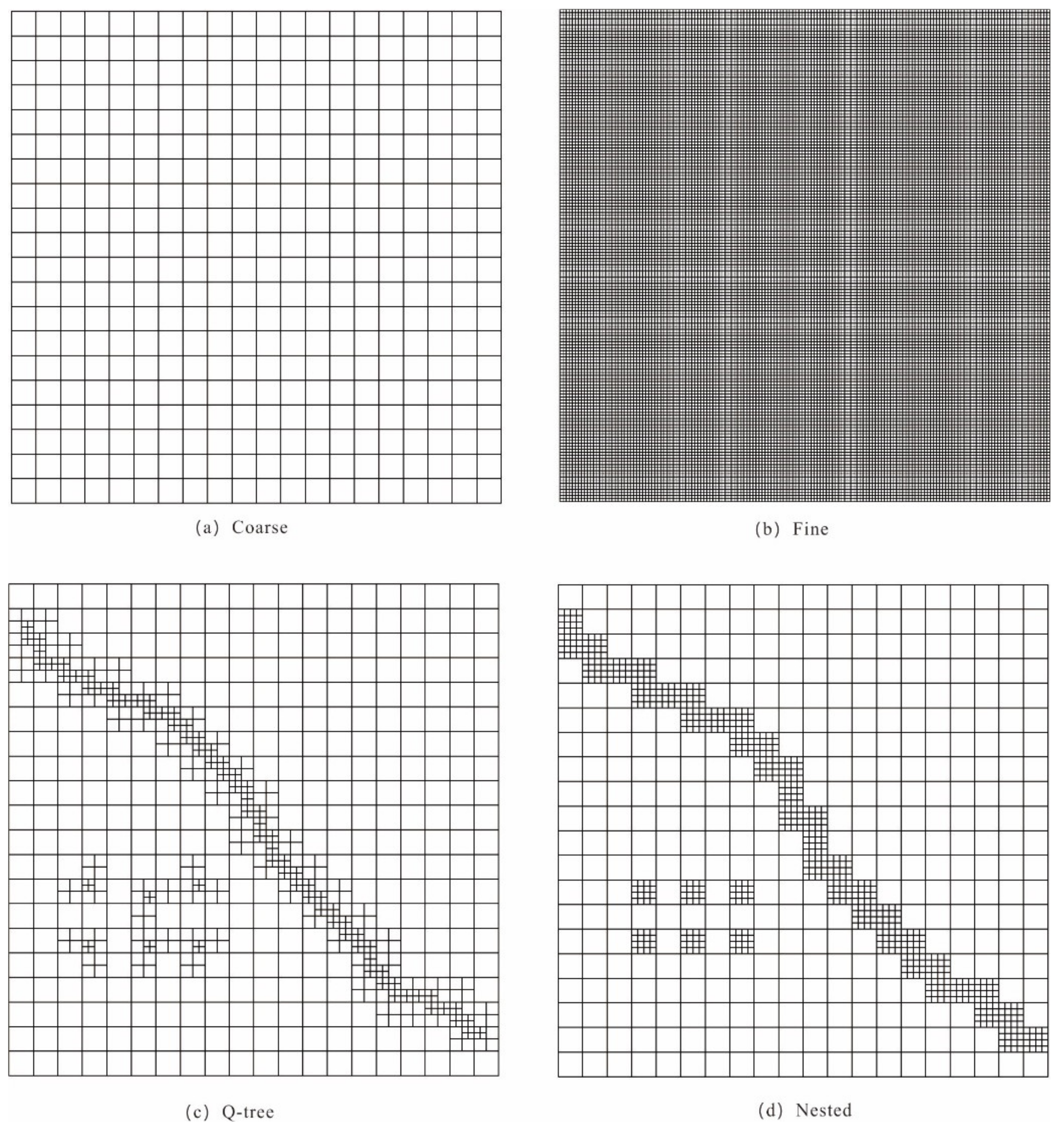
Scheme 1 (Coarse Grid): We globally divided the model into 1200 grid cells of 500 m × 500 m to serve as a reference model without grid refinement, as illustrated in Figure 3a.
Scheme 2 (Fine Grid): We divided the model into 1,228,800 grid cells of 15.625 m × 15.625 m. This scheme served as a base model with a more precise characterization of groundwater movement than Scheme 1 and is illustrated in Figure 3b.
Scheme 3 (Q-tree Grid): Based on Scheme 1, we refined the grids near the river (3-degree refinement). The smallest grid cell was 125 m × 125 m and the cell size gradually increased to 500 m × 500 m away from both sides of the river. The total number of grid cells was 2586, as shown in Figure 3c. We also conducted a 6-degree refinement, for which the smallest grid cell size was 15.625 m × 15.625 m, to compare the computational efficiency of the four schemes.
Scheme 4 (Nested Grid): Based on Scheme 1, we locally refined the grids near the river, where the smallest grid cell was 125 m × 125 m. The grid cells in the other regions were 500 m × 500 m. There were 3135 grid cells in total, as illustrated in Figure 3d. Also, the grid size was further reduced to 15.625 m × 15.625 m to compare the computational efficiency of the four schemes.
3.3. Simulation Scenarios
We considered two simulation scenarios, with and without river recharge. The scenarios were simulated holding all other conditions fixed, except the river recharge into groundwater. We adopted the scheme 2 as the base model. Use the other schemes simulation results to compare the effects of the two unstructured grid refinement methods on simulation. These include flow fields, groundwater levels, and groundwater flow, as well as the computational time, which was used to analyze the computational efficiency of the different schemes.
4. Results and Discussion
4.1. Computational Efficiency
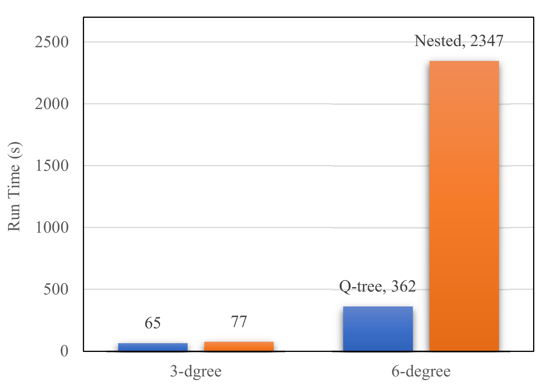
Computation efficiency is a priority in the application of groundwater models [24]. Using an excessive number of grids in the model construction can easily result in low model calculation efficiencies or even stop the model from running, creating considerable difficulties in grid refinement. We compared the computation efficiencies of the four schemes in this study. The computations were performed using a 1.8 GHz, 4-core, 8 G RAM processor. The calculation results are summarized in Table 1 and Figure 4.
The fine grid model had a higher resolution than the coarse grid model. However, an excessive number of grids were generated, and the whole simulation took 5 h and generated 40 G results files that took up a large amount of computer storage space. In comparison, the two unstructured grid models only refined the grid near the river, resulting in a modest increase in the grid number to 2586 and 3135 from 1200 for the coarse grid. The smallest grid cells for the unstructured grid models were 125 m in size, and the computation times were a little larger than for the coarse grid model.
A comparison of the two unstructured grids showed that the 3-degree Q-tree model, in which the smallest grid cell was 125 m in size, was 18% more efficient than the nested grid model in terms of the computation time. This result was obtained because the nested grid refinement scheme uniformly refined the grids along the river, whereas the gradual grid generation scheme of the Q-tree model produced fewer grid cells. In addition, the computation time of the 6-degree Q-tree model, in which the local smallest grid cell was 15.625 m, was only 15% of that of the nested grid model, thus saving 85% of the computation time. This result illustrates that the higher the refinement degree is, the more efficient the Q-tree grid refinement method is. Thus, the Q-tree method offers the advantage of multi-degree refinement over the nested grid scheme.
4.2. Comparison of Simulated Flow Fields
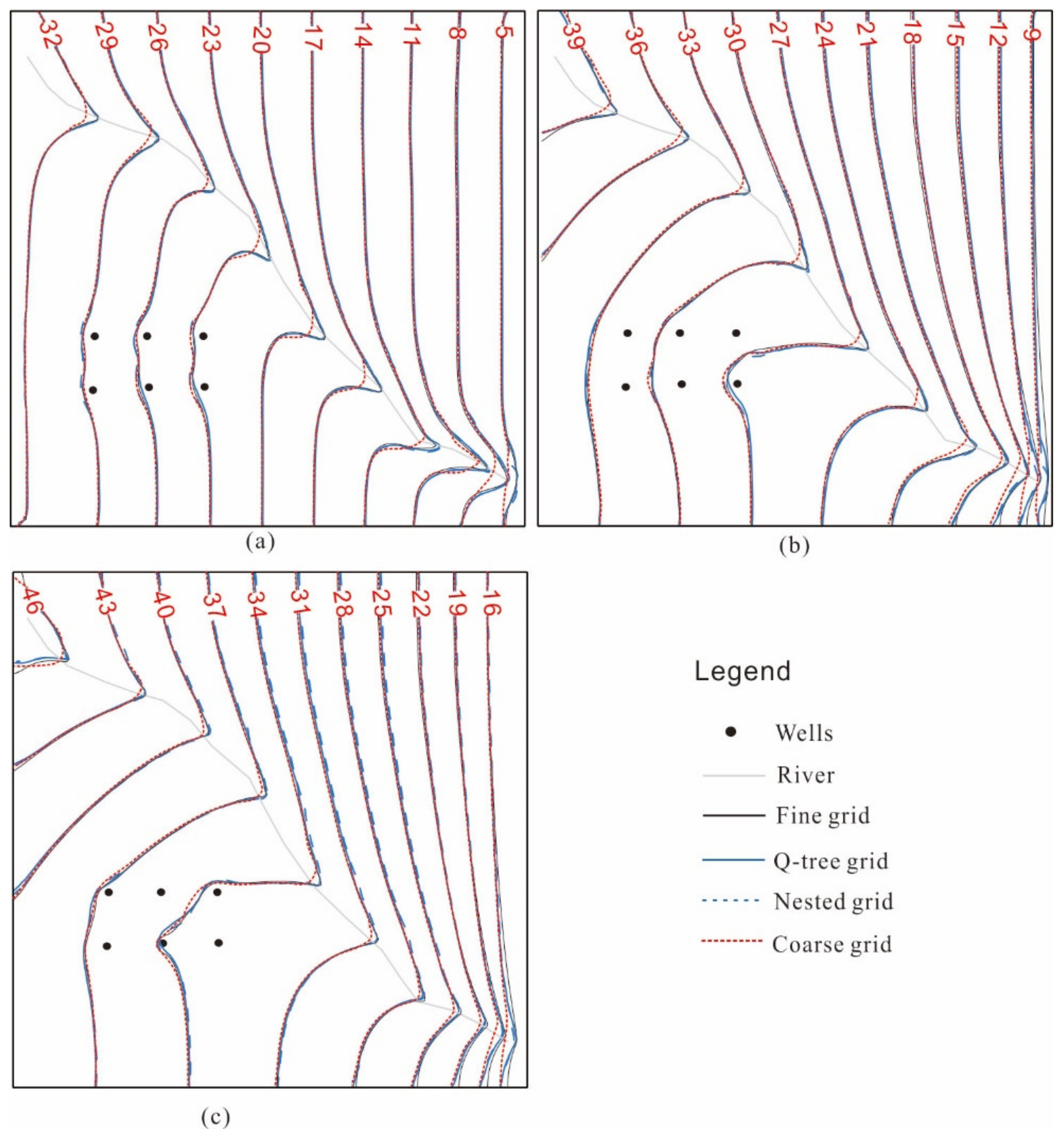
Figure 5 shows the groundwater levels simulated using the four schemes for three simulation periods (1, 6, and 12 months). The simulated groundwater levels are generally consistent, and the groundwater levels overlap in most regions. However, river recharge of groundwater creates water hills along the river, resulting in significant differences in the simulated flow field morphology near the river obtained using the four schemes. We observed large errors in the coarse grid simulation results, especially during the early recharge period, which has a relatively small influence range.
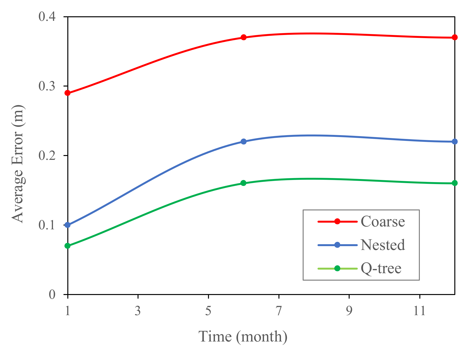
We used a quantitative assessment method to accurately compare the differences among the four simulated flow fields. We used the fine grid model (Scheme 2) as a standard to calculate the simulation errors for the other schemes within 500 m of the river (Table 2, Figure 6). The results showed that the coarse grid model yielded the highest simulation error, followed by the nested grid model, whereas the Q-tree model produced the smallest simulation error. For instance, the simulation errors obtained using the coarse, nested and Q-tree grids over a 12-month simulation period were 0.38 m, 0.24 m, and 0.17 m, respectively. The simulations errors for regions within 500 m of the river trended upwards with increasing time, but the magnitude of the increase was generally slightly lower for the Q-tree model than for the nested grid model.
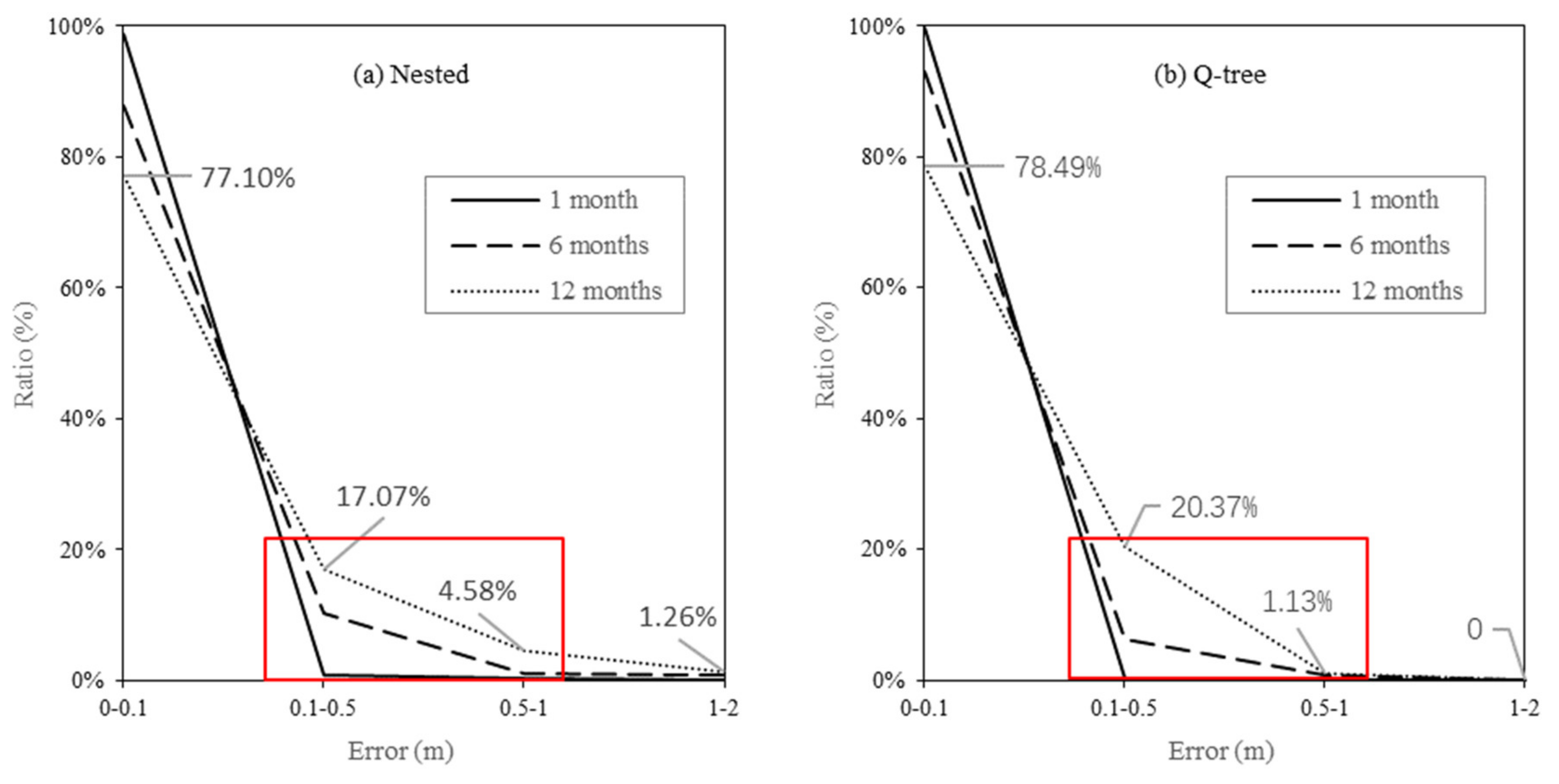
Figure 7 shows the probability distributions of errors in the simulated groundwater levels obtained using the two unstructured grid models within 500 m of the river. After 1 month, the simulation errors are similar for both models and almost remain within 0.1 m (the corresponding probabilities are 98.93% and 99.77%). The probability of generating >0.1 m errors in the simulated groundwater levels using the two models gradually increases with the simulation time, i.e., 6 or 12 months. After 12 months, the probability of generating >0.5 m errors by the nested grid is 5.2 times that by the Q-tree grid model. After 12 months, >1 m errors start to appear in the nested grid model, whereas the errors produced during the whole Q-tree scheme simulation always remain below 1 m. This result illustrates the advantage of using the Q-tree model for long-term simulation.
4.3. Simulated Relative Rise of Groundwater Level
4.3.1. Comparison of Different Schemes
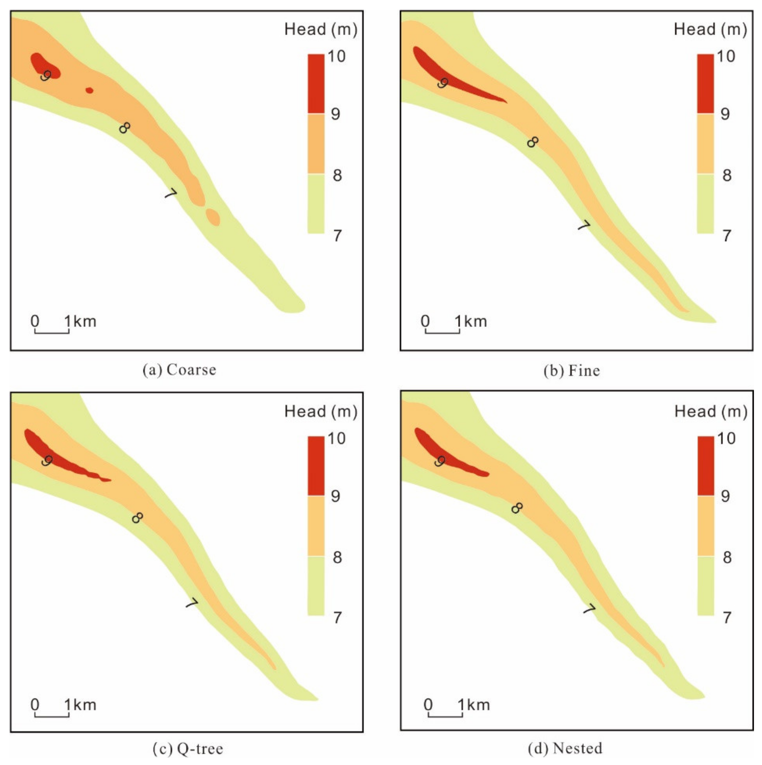
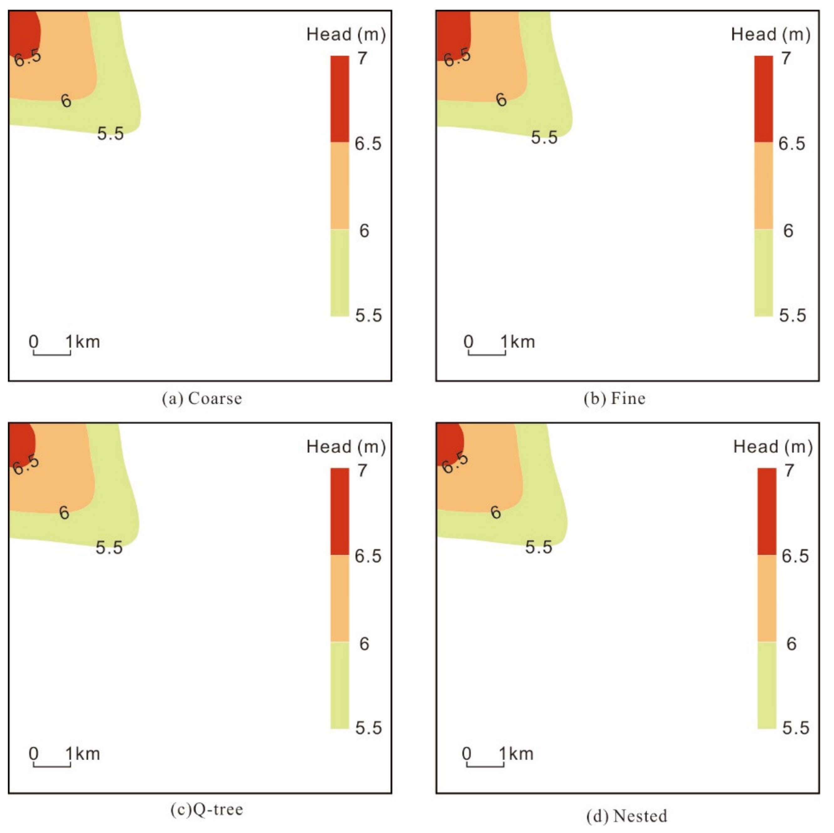
Figure 8 and Figure 9 illustrate the contour of simulated relative rises of groundwater level within the recharge scenario (i.e., the simulated groundwater level within the recharge scenario minus the simulated groundwater level within the non-recharge scenario). Overall, the four schemes yielded quite similar simulation results: the contour was distributed along the river as bands, and the upper reaches of the recharge river were quite significantly affected, whereas the effect decreased toward the lower reaches.
However, the simulation results shown in Figure 8a for the coarse grid model and Figure 8b for the base model differ in terms of the morphology of the contour for the phreatic aquifer. The former is mainly characterized by rough contour lines, and a discontinuity even appears, e.g., the 8 m and 9 m contour lines. The area contained within the 9 m contour line in the base model is 0.74 km2, while the corresponding numbers given by the Q-tree and nested models are 0.68 km2 and 0.66 km2, respectively, both of which are quite close to the value given by the base model. By comparison, the corresponding area for the coarse grid model is only 0.33 km2, which is 55% smaller than that for the base model. Thus, the results show that the two unstructured grid schemes have higher simulation precisions and can characterize the morphology of contour lines in more detail than the coarse grid model.
In summary, the unstructured grid refinement method can more effectively increase the simulation precision than the coarse grid model. This advantage is especially significant for regions near rivers with relatively high groundwater level rises, whereas there is a relatively small increase in the simulation precision for regions far from rivers and for confined aquifers.
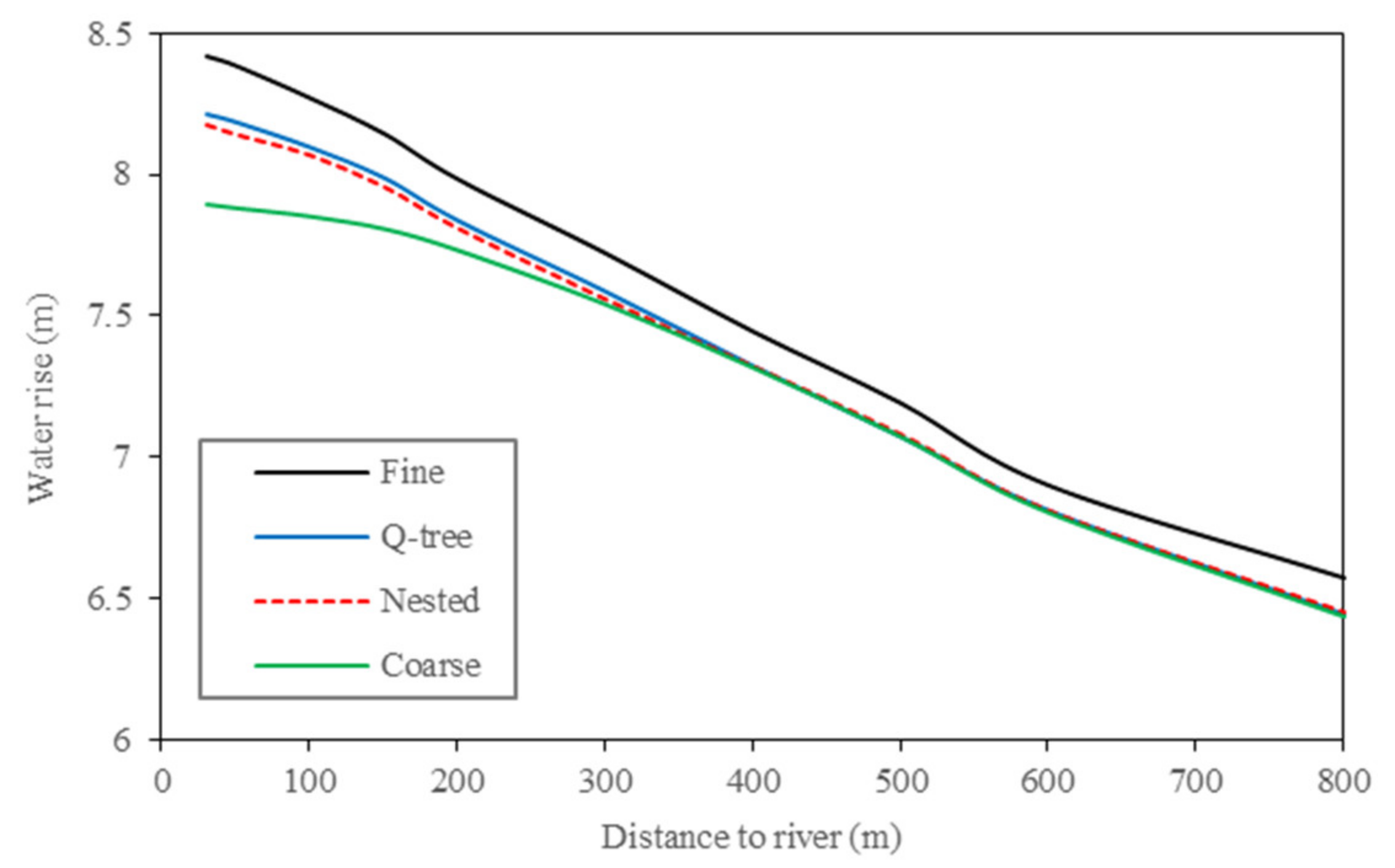
We calculated the average relative rise of groundwater level at different distances from the river to directly illustrate the differences between the four schemes, where the statistical calculations were taken to be the end of the simulation period. Figure 10 shows that the simulated relative rise of groundwater level continuously decreases, and the influence of river recharge decreases with increasing distance from the river for all four schemes. The simulation results of the two unstructured grid schemes are almost consistent with that of the coarse grid model for regions more than 300 m from the river. However, within 300 m of the river, the results of the two unstructured grid schemes are closer to the base model result than the coarse grid model result. Within 30 m from the river, the relative rise of groundwater level obtained using the base model is 8.41 m compared to the two unstructured grid refinement model results of 8.21 m and 8.17 m and the significantly lower coarse grid model result of only 7.89 m. Such a large difference (0.52 m) can lead to an inaccurate assessment of recharge, especially near the river.
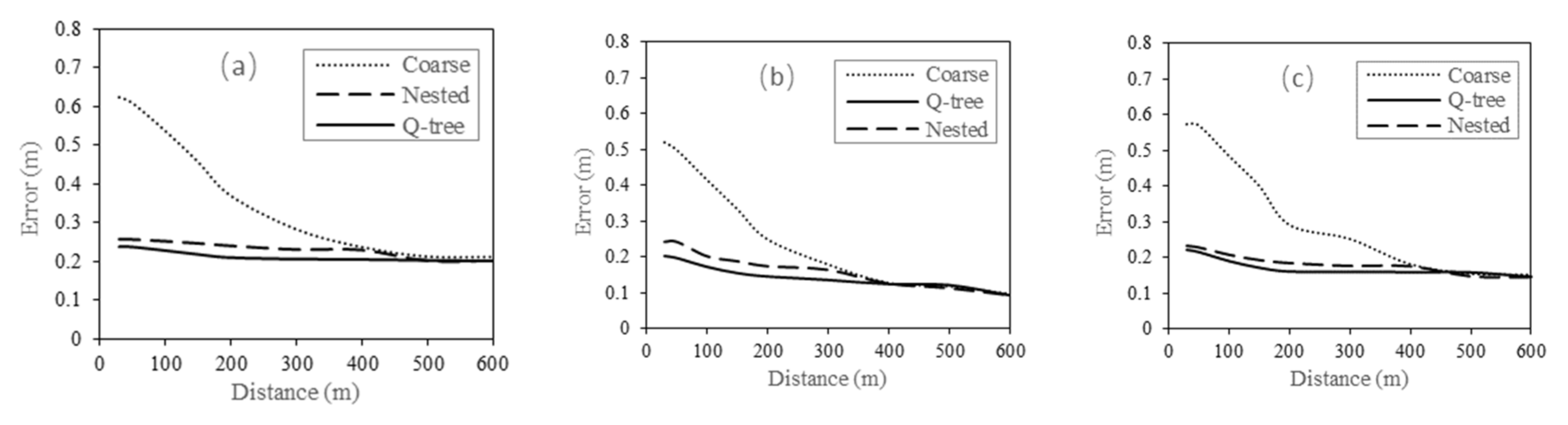
4.3.2. Effect of Boundary Conditions on Simulation Errors
Boundary condition setting is crucial in numerical simulations. The results presented above were all obtained by setting the boundary on the west as a Neumann boundary. Figure 11 presents a comparison of the simulation errors produced under different boundary conditions. The simulation errors obtained using different schemes exhibit quite similar variation trends overall under the three boundary conditions. All the simulation errors are comparable for distances more than 400 m from the river. Within 400 m of the river, the two unstructured grid schemes produce significantly smaller simulation errors than the coarse grid scheme. Thus, the advantages offered by the two unstructured grid schemes becomes more significant upon approaching the river. Our results demonstrate that the unstructured grid refinement method has high simulation precision independent of boundary conditions. Furthermore, the errors of the Q-tree grid scheme are overall smaller than those of the nested grid scheme by approximately 0.01–0.04 m. That is, the Q-tree grid refinement method has a slightly higher simulation precision than the nested grid refinement method.
4.3.3. Effect of Refinement Degree on Simulation Error
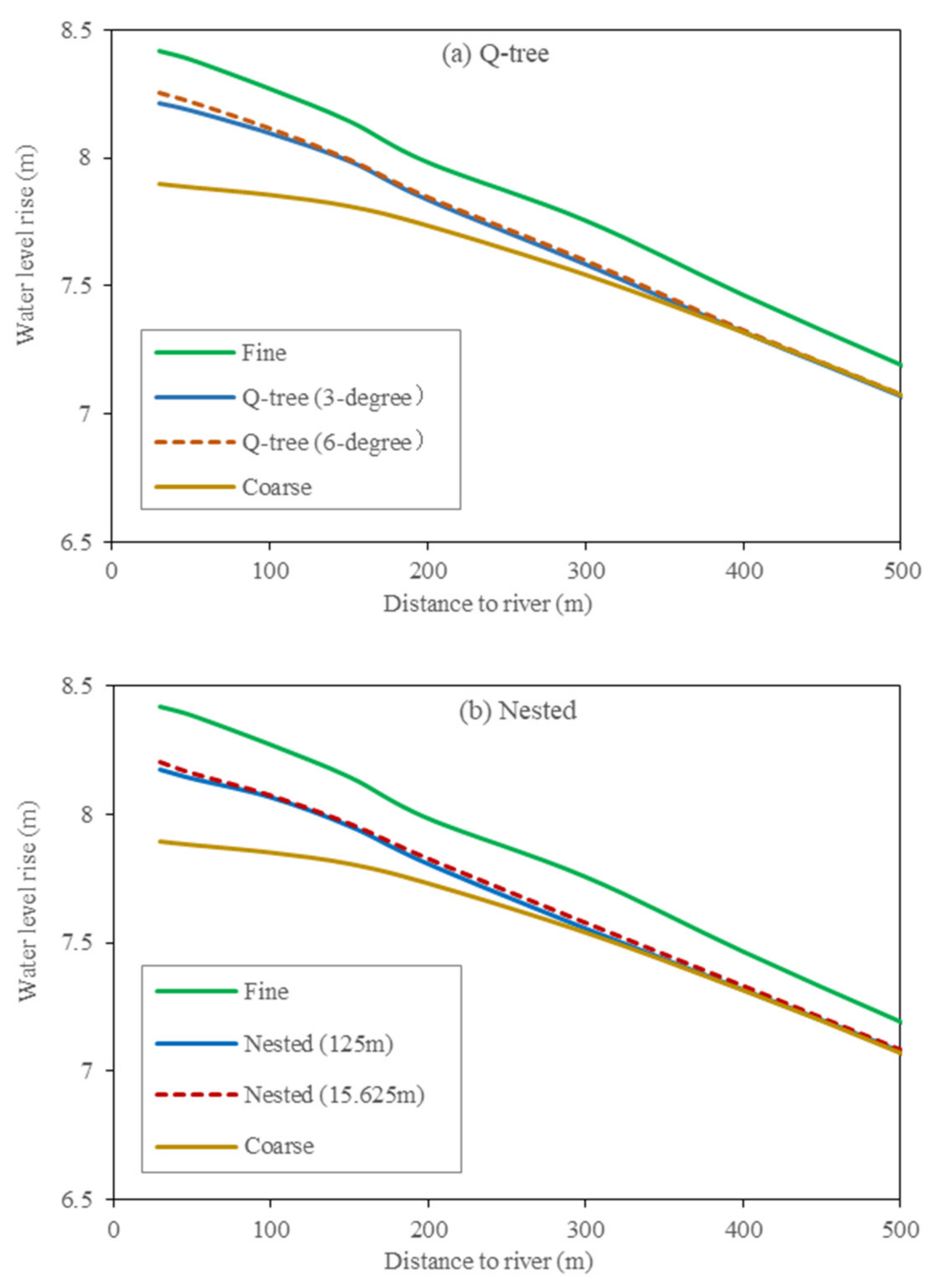
The Q-tree and nested methods can refine unstructured grids by multiple degrees. The smallest grid cell is 125 and 15.625 m after 3- and 6-degree refinement by the Q-tree method, respectively. Nested grids can also perform similar refinement. Figure 12 shows quite similar 6- and 3-degree refinement results obtained using the Q-tree method and the nested grid model. The additional refinement increases the simulated water levels obtained using the Q-tree method and the nested grid model by only 0.04 m and 0.03 m, respectively. These increases become smaller with the increasing distance from the river course. However, the additional refinement considerably increases the number of grid cells by 42 times for the nested scheme and by 6 times for the Q-tree scheme. The additional refinement is clearly not useful for increasing simulation precision. However, when the refined grid reaches a size of 15.625 m, the grid number of the nested scheme is 7 times that for the Q-tree scheme. That is, the Q-tree scheme exhibits superior performance for multi-degree refinement because the number of grids is smaller than that of the nested scheme without compromising the simulation precision.
4.4. Differences in Groundwater Flow
As previously discussed, different grid generation schemes produce different simulated groundwater levels near the river, which in turn affects the simulated groundwater runoff. Table 3 summarizes the groundwater flow across the distance of 200 m from the river. Compared to the base model result, the simulated groundwater flow volume based on the unrefined coarse grid scheme result is 14.9% lower, whereas the corresponding values of the nested and Q-tree scheme are only 4.2% and 3.6% lower, respectively. This result shows that the unstructured refinement methods, especially the Q-tree refinement method, has advantage in terms of the simulation of groundwater flow.
5. Conclusions
We compared the flow fields and groundwater level changes at different distances from the river as well as the groundwater flow and model computation time simulated by different grid generation schemes. The results showed that the two unstructured refinement schemes significantly improved the simulation precision and more accurately characterized groundwater level changes from river recharge. The improvement was especially significant near the river and remained consistent under different boundary conditions. In addition, the simulation precision for the groundwater flow obtained using the two unstructured grid schemes was significantly enhanced compared to that of the coarse grid scheme.
The Q-tree grid scheme generated fewer grid cells, required less computation time, and performed more effectively than the nested grid scheme. Additionally, the higher the refinement degree was, the more significant the advantages were. However, a comparison of 3- and 6-degree refinement modeling results showed that increasing the refinement degree did not significantly improve the simulation precision.
In conclusion, the Q-tree grid refinement method has a relatively high simulation precision and computation efficiency for simulating the effects of river recharge on groundwater. Hence, the Q-tree model is recommended as a local grid refinement method, offering significant advantages. However, there are still some differences between the unstructured refinement model results and the base model result. A trade-off between the computational efficiency and precision is required in the construction of practical models. The connection between river and groundwater in this study is not successive. The surface water level is much higher than groundwater level. A further study could be conducted when the connection between river and groundwater become successive.
Author Contributions
Conceptualization, Q.H. and W.C.; methodology, Q.H.; software, W.C.; validation, Q.H. and W.C.; formal analysis, W.C.; investigation, W.C.; resources, Q.H.; data curation, W.C.; writing—original draft preparation, W.C.; writing—review and editing, Q.H.; visualization, W.C.; supervision, Q.H.; project administration, Q.H.; funding acquisition, Q.H. All authors have read and agreed to the published version of the manuscript.
Funding
This research was funded by the Natural Science Foundation of China, grant number 41702282, and the China Geological Survey Project, grant number DD20160238, DD20190303.
Acknowledgments
The authors would like to thank the staff of the General Institute of Water Resources and Hydropower Planning and Design as well as the Ministry of Water Resources of China for their support and interest in this work.
Conflicts of Interest
The authors declare no conflict of interest.
References
- Fei, Y.H.; Cui, G.B. Development and Problems: Research on Artificial Adjustment of Groundwater Storage. J. China Hydrol. 2006, 26, 10–14. [Google Scholar]
- Jonoski, A.; Zhou, Y.X.; Nonner, J.; Meijer, S. Model-aided design and optimization of artificial recharge-pumping systems. Int. Assoc. Sci. Hydrol. Bull. 1997, 42, 937–953. [Google Scholar] [CrossRef]
- Jarraya Horriche, F.; Benabdallah, S. Assessing Aquifer Water Level and Salinity for a Managed Artificial Recharge Site Using Reclaimed Water. Water 2020, 12, 341. [Google Scholar] [CrossRef] [Green Version]
- Dillon, P.; Fernández Escalante, E.; Megdal, S.B.; Massmann, G. Managed Aquifer Recharge for Water Resilience. Water 2020, 12, 1846. [Google Scholar] [CrossRef]
- Chen, F.; Ding, Y.Y.; Li, Y.Y.; Li, W.; Tang, S.N.; Yu, L.L.; Liu, Y.Z.; Yang, Y.; Li, J.; Zhang, Y. Practice and Thinking of Groundwater Overdraft Restoration in North Plain China. South-to-North Water Transf. Water Sci. Technol. 2020, 18, 191–198. [Google Scholar]
- Gupta, S.K.; Cole, C.R.; Pinder, G.F. A Finite-Element Three-Dimensional Groundwater (FE3DGW) Model for a Multiaquifer System. Water Resour. Res. 1984, 20, 553–563. [Google Scholar] [CrossRef]
- Guo, W.X. Transient groundwater flow between reservoirs and water-table aquifers. J. Hydrol. 1997, 195, 370–384. [Google Scholar] [CrossRef]
- Hao, Q.C.; Shao, J.L.; Hua, X.Z.; Zhang, X.G. A Study of the artificial adjustment of groundwater storage of the Yongding River alluvial fan in Beijing. Hydrogeol. Eng. Geol. 2012, 39, 12–18. [Google Scholar]
- Niswonger, R.G.; Morway, E.D.; Triana, E.; Huntington, J.L. Managed aquifer recharge through off-season irrigation in agricultural regions. Water Resour. Res. 2017, 53, 6970–6992. [Google Scholar] [CrossRef]
- Hao, Q.C.; Shao, J.L.; Cui, Y.L.; Zhang, Q.L.; Huang, L.X. Optimization of groundwater artificial recharge systems using a genetic algorithm: A case study in Beijing, China. Hydrogeol. J. 2018, 26, 1749–1761. [Google Scholar] [CrossRef]
- Yao, Y.Y.; Zheng, C.M.; Liu, J.; Cao, G.L.; Xiao, H.L.; Li, H.T.; Li, W.P. Conceptual and numerical models for groundwater flow in an arid inland river basin. Hydrol. Process. 2015, 29, 1480–1492. [Google Scholar] [CrossRef]
- Panday, S.; Langevin, C.D.; Niswonger, R.G.; Ibaraki, M.; Hughes, J.D. U.S. Geological Survey, MODFLOW–USG Version 1: An Unstructured Grid Version of MODFLOW for Simulating Groundwater Flow and Tightly Coupled Processes Using a Control Volume Finite-Difference Formulation; U.S. Geological Survey: Washington, DC, USA, 2013; p. 5.
- Krcmar, D.; Sracek, O. MODFLOW-USG: The New Possibilities in Mine Hydrogeology Modelling (or What is Not Written in the Manuals). Mine Water Environ. 2014, 33, 376–383. [Google Scholar] [CrossRef]
- Naser, S.; Masoud, M.N.; Javad, F. A 3D unstructured triangular numerical algorithm for simultaneous effects of fluid density variation and water table gradient in saturated porous media. J. Hydrol. 2019, 568, 479–491. [Google Scholar]
- Kumar, C.P. An overview of commonly used groundwater modelling software. Int. J. Adv. Res. Sci. Eng. Technol. 2019, 6, 7854–7865. [Google Scholar]
- Samet, H. The Quadtree and Related Hierarchical Data Structures. ACM Comput. Surv. 1984, 16, 187–260. [Google Scholar] [CrossRef] [Green Version]
- Yerry, M.A. A Modified Quadtree Approach To Finite Element Mesh Generation. IEEE Comput. Graph. 1983, 3, 39–46. [Google Scholar] [CrossRef]
- Rogers, B.; Fujihara, M.; Borthwick, A.G.L. Adaptive Q-tree Godunov-type scheme for shallow water equations. Int. J. Numer. Meth. Fl. 2015, 35, 247–280. [Google Scholar] [CrossRef]
- Liu, X.D.; Hua, Z.L.; Zhao, Y.P. Quad-Tree Meshes Based Godunov-Type 2-D Flow Numerical Model. J. Hohai Univ. (Nat. Sci.) 2002, 30, 6–10. [Google Scholar]
- Đorđije, B.; Dušan, P.; Dragoljub, B.; Jelena, R. Hydrodynamic analysis of radial collector well ageing at Belgrade well field. J. Hydrol. 2020, 582, 124463. [Google Scholar]
- Mehl, S.W.; Hill, M.C. MODFLOW–LGR—Documentation of Ghost Node Local Grid Refinement (LGR2) for Multiple Areas and the Boundary Flow and Head (BFH2) Package; 6-A44; U.S. Geological Survey: Reston, VA, USA, 2013; p. 54.
- Khan, M.R.; Koneshloo, M.; Knappett, P.S.; Ahmed, K.M.; Bostick, B.C.; Mailloux, B.J.; Mozumder, R.H.; Zahid, A.; Harvey, C.F.; Van Geen, A. Megacity pumping and preferential flow threaten groundwater quality. Nat. Commun. 2016, 7, 1–8. [Google Scholar] [CrossRef]
- Forghani, A.; Peralta, R.C. Transport modeling and multivariate adaptive regression splines for evaluating performance of ASR systems in freshwater aquifers. J. Hydrol. 2017, 553, 540–548. [Google Scholar] [CrossRef]
- Asher, M.J.; Croke, B.F.W.; Jakeman, A.J.; Peeters, L.J.M. A review of surrogate models and their application to groundwater modeling. Water Resour. Res. 2015, 51, 5957–5973. [Google Scholar] [CrossRef]
Figure 1.
Comparison of Q-tree and nested grids refinement method.

Figure 2.
Structure and setup for managed aquifer recharge model.

Figure 3.
Schematic of four grid generation schemes.

Figure 4.
Comparison of the computation times of two unstructured grid schemes.

Figure 5.
Comparison of simulated groundwater level (a): 1 month; (b): 6 months; and (c): 12 months, unit of number at the contour lines is m.
Figure 5.
Comparison of simulated groundwater level (a): 1 month; (b): 6 months; and (c): 12 months, unit of number at the contour lines is m.

Figure 6.
Comparison of simulation errors obtained using different models.

Figure 7.
Comparison of error probability between two unstructured grid schemes.

Figure 8.
Simulated relative rise of groundwater level of the phreatic aquifer.

Figure 9.
Simulated relative rise of groundwater level of the confined aquifer.

Figure 10.
Comparison of relative rise of groundwater level at different distances from the river.

Figure 11.
Simulation errors in relative rise of groundwater level under different boundary conditions (a): Dirichlet; (b): Neumann; and (c): General.
Figure 11.
Simulation errors in relative rise of groundwater level under different boundary conditions (a): Dirichlet; (b): Neumann; and (c): General.

Figure 12.
Comparison of relative rise of groundwater level under different refinement degrees.


Table 1.
Comparison of computation time for different models.
| Grid Type | Number of Cells | Computation Time (s) |
|---|---|---|
| Coarse Grids | 1200 | 32 |
| Q-tree Grids (3-degree refinement) | 2586 | 65 |
| Nested Grids (local 125 m) | 3135 | 77 |
| Q-tree Grids (6-degree refinement) | 15,771 | 362 |
| Nested Grids (local 15.625 m) | 133,167 | 2347 |
| Fine Grids | 1,228,800 | 18,126 |
Table 2.
Comparison of simulation errors obtained using different models.
| Period | Grid Generation Scheme | Simulation Error (m) |
|---|---|---|
| 1 Month | Coarse Grid | 0.29 |
| Nested Grid | 0.10 | |
| Q-tree Grid | 0.07 | |
| 6 Months | Coarse Grid | 0.37 |
| Nested Grid | 0.22 | |
| Q-tree Grid | 0.16 | |
| 12 Months | Coarse Grid | 0.38 |
| Nested Grid | 0.24 | |
| Q-tree Grid | 0.17 |
Table 3.
Comparison of groundwater flow obtained under different schemes.
| Schemes | Flow Volume (104 m3/d) | Error (Percentage) |
|---|---|---|
| Fine Grids | 16.8 | / |
| Q-tree Grids | 16.2 | −3.6% |
| Nested Grids | 16.1 | −4.2% |
| Coarse Grids | 14.3 | −14.9% |
Publisher’s Note: MDPI stays neutral with regard to jurisdictional claims in published maps and institutional affiliations. |
© 2020 by the authors. Licensee MDPI, Basel, Switzerland. This article is an open access article distributed under the terms and conditions of the Creative Commons Attribution (CC BY) license (http://creativecommons.org/licenses/by/4.0/).
Share and Cite
MDPI and ACS Style
Cui, W.; Hao, Q. Comparing Q-Tree with Nested Grids for Simulating Managed River Recharge of Groundwater. Water 2020, 12, 3516. https://doi.org/10.3390/w12123516
AMA Style
Cui W, Hao Q. Comparing Q-Tree with Nested Grids for Simulating Managed River Recharge of Groundwater. Water. 2020; 12(12):3516. https://doi.org/10.3390/w12123516
Chicago/Turabian StyleCui, Weizhe, and Qichen Hao. 2020. "Comparing Q-Tree with Nested Grids for Simulating Managed River Recharge of Groundwater" Water 12, no. 12: 3516. https://doi.org/10.3390/w12123516
Note that from the first issue of 2016, this journal uses article numbers instead of page numbers. See further details here.