Article

Evaluation of AnnAGNPS Model for Runoff Simulation on Watersheds from Glaciated Landscape of USA Midwest and Northeast

1
Department of Geosciences, University of Rhode Island, Kingston, RI 02881, USA
2
Department of Natural Resource Sciences, University of Rhode Island, Kingston, RI 02881, USA
3
Sustainable Resources Management Department, The State University of New York College of Environmental Science and Forestry, Syracuse, NY 13210, USA
4
USDA-ARS National Sedimentation Laboratory, Oxford, MS 38655, USA
*
Authors to whom correspondence should be addressed.
Water 2020, 12(12), 3525; https://doi.org/10.3390/w12123525
Submission received: 15 October 2020 / Revised: 21 November 2020 / Accepted: 8 December 2020 / Published: 15 December 2020

Abstract

:
Runoff modeling of glaciated watersheds is required to predict runoff for water supply, aquatic ecosystem management and flood prediction, and to deal with questions concerning the impact of climate and land use change on the hydrological system and watershed export of contaminants of glaciated watersheds. A widely used pollutant loading model, Annualized Agricultural Non-Point Source Pollution (AnnAGNPS) was applied to simulate runoff from three watersheds in glaciated geomorphic settings. The objective of this study was to evaluate the suitability of the AnnAGNPS model in glaciated landscapes for the prediction of runoff volume. The study area included Sugar Creek watershed, Indiana; Fall Creek watershed, New York; and Pawcatuck River watershed, Rhode Island, USA. The AnnAGNPS model was developed, calibrated and validated for runoff estimation for these watersheds. The daily and monthly calibration and validation statistics (NSE > 0.50 and RSR < 0.70, and PBIAS ± 25%) of the developed model were satisfactory for runoff simulation for all the studied watersheds. Once AnnAGNPS successfully simulated runoff, a parameter sensitivity analysis was carried out for runoff simulation in all three watersheds. The output from our hydrological models applied to glaciated areas will provide the capacity to couple edge-of-field hydrologic modeling with the examination of riparian or riverine functions and behaviors.

1. Introduction

Excess nutrient (primarily nitrogen and phosphorus) losses from agricultural watersheds in glaciated settings of the Midwest and Northeast of USA are one of the greatest water quality problems tied to modern agriculture [1,2,3,4,5,6]. These water quality problems include eutrophication, harmful algae blooms, and fish kills in the Gulf of Mexico, the Chesapeake Bay, the Hudson River Estuary, and other coastal areas [7,8,9,10]. A substantial body of research on riparian zone hydrology and biogeochemistry has shown that riparian zones can serve as efficient best management practices (BMPs) for nutrient removal [11,12].
The functional efficiency of nutrient removal in a riparian zone can vary widely depending on the characteristics within the riparian zone (e.g., vegetation, soil texture, depth to water table) and on its location in the landscape, timing, characteristics and extent of contaminant and hydrologic loading and its hydrogeomorphic setting [11,12,13,14,15,16,17,18,19]. Thus, it is significant to explore the relationships between the landscape-generated “edge-of-field” waterborne losses and riparian functioning to improve riparian design and to better quantify the extent of treatment within riparian zones [20]. Given the expense and time associated with empirical studies, simulation models offer the capacity to examine riparian zone performance across many different soils, topography settings, agricultural practices and climatic conditions.
The Riparian Ecosystem Management Model (REMM) [21,22] has been used in non-glaciated settings, primarily in a region extending from Texas to the Atlantic coast to explore the pollution abatement of riparian zones. In companion studies we are examining the efficacy of the REMM model for use in glaciated settings of the Northeast and Midwest, USA. Over the past two decades, the authors of this manuscript have generated an extensive, empirically derived data base on riparian zone structure and functions from three glaciated watersheds—located over a 1400 km east–west band encompassing about 3 degrees of latitude (39.72° to 42.44° N). All of these watersheds lack empirical data on edge-of-field overland runoff. In contrast to the piedmont and coastal plains where REMM has been used, the flux of water and water-borne contaminants in these glaciated regions are driven by differences in the magnitude and timing of snowmelt, the frequency of freeze–thaw phenomena, lower evapotranspiration and the varied soils and geomorphology (e.g., hilly, low permeability till that co-occur with flat, high permeability stratified drift landforms and narrow bands of alluvial soils) that often exist within small watersheds. [23] demonstrated that there were higher average annual runoff and higher seasonal (winter, spring, fall) runoff loads in northeastern glaciated watersheds than non-glaciated watersheds.
Here, we evaluate the AnnAGNPS (Annualized Agricultural Non-Point Source) [24,25] model for its efficacy to predict runoff from glaciated, upland areas to riparian buffers—a key requirement for riparian zone models such as the REMM model. AnnAGNPS is a distributed model that can assess the continuous hydrologic and water quality responses of watersheds to daily weather conditions in a variety of soils, land uses and land covers. AnnAGNPS has been successfully used in several states of USA, such as Illinois [26], Indiana [27], Mississippi [28,29], Georgia [30], Kansas [31], New York [32]. Globally, AnnAGNPS has been effectively used in numerous parts of the world in recent years, including Brazil [33], Spain [34], Nigeria [35], Italy [36,37,38], Canada [39], Australia [40], Nepal [41], China [42], Belgium [43], Malaysia [44], and Saint Lucia [45]. AnnAGNPS has been implemented in all of these studies to predict runoff, sediment, and pollutant loadings under various environmental conditions representing different watersheds. AnnAGNPS model was selected for this study since the model can generate estimates of “edge-of-field” losses to specific downgradient cells, such as riparian zones, which enables the output of AnnAGNPS to serve as input to riparian buffer models. AnnAGNPS divides a watershed into a number of cells (characterized by similar land and soil properties) of various sizes, and runoff and contaminants are routed from these cells into the associated reaches, and the model either deposits pollutants within the stream channel system or transports them out of the watershed. The cell-based structure was not available in a number of other commonly used water quality models (e.g., Chemicals, Runoff, and Erosion from Agricultural Management Systems (CREAMS), Groundwater Loading Effects on Agricultural Management Systems (GLEAMS), Hydrological Simulation Program—FORTRAN (HSPF) and Soil & Water Assessment Tool (SWAT), which lack or are limited in the extent of spatially explicit simulations within and between locations at the field and watershed scale. For example, the SWAT model divides a watershed into sub-watershed or hydrological response units (HRUs) exhibiting homogenous land, soil and slope characteristics instead of a fine-resolution grid network. This limits its incorporation of spatial variability (very crucial for riparian zone) in simulating the hydrologic dynamics that drive many functions of riparian buffers.
Based on the review of literature, we found that AnnAGNPS has not been applied in watersheds of glacial geomorphic settings, such as our studied watersheds, to model runoff generation and other hydrological processes. The objective of this study was to evaluate the suitability of the AnnAGNPS model in glaciated landscapes for the estimation of runoff quantity. The geomorphic setting, i.e., the glaciated landscape, makes the AnnAGNPS model application unique in this study. Our study area included Sugar Creek watershed in Indiana, Fall Creek watershed in New York and Pawcatuck River watershed in Rhode Island. All the watersheds are located in a glacial geomorphic setting.
Specifically, this paper aims to: (i) evaluate the performance of the AnnAGNPS model in simulating the runoff volume at three separate watersheds with glacial setting; (ii) improve the model’s runoff prediction capacity through calibration; (iii) validate the model’s runoff prediction with the improved calibrated parameters; (iv) conduct a parameter sensitivity analysis for runoff simulation; (v) conduct an analysis of the spatial distribution of runoff depth for three watersheds; (vi) provide a discussion of the model’s performance in order to estimate event peak discharge.

2. Materials and Methods
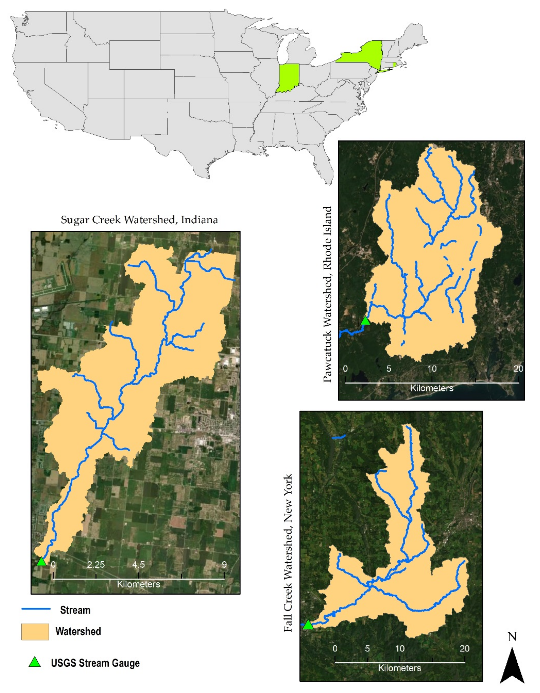
2.1. Study Area

Three watersheds from three different states were modeled for this study. Sugar Creek watershed (39°43′21″ N, 85°53′23″ W), a part of the White River watershed in central Indiana, is about 69 km2 (Figure 1). The elevation of the watershed ranges from 241 m to 280 m, and the topography is nearly flat. The watershed consists largely of tile-drained agricultural lands (88% of the total watershed area, representative of agro-ecosystems of the glacial till plains from US Midwest [46]. This watershed is dominated by poorly drained soils where artificial drainage is usually used to lower the water table [47]. For the past 20 years, agricultural practices have been dominated by a corn/soybean rotation with either conventional or conservation tillage systems [48]. The temperature in the watershed is moderate, ranging from a 30-year (1982–2011) mean of 22.7 °C in summer to a mean of −1.4 °C in winter (Parameter-elevation Regressions on Independent Slopes Model (PRISM) Climate Group, accessed on 4 May 2019). The 30 years (1982–2011) average annual precipitation is approximately 1105.0 mm, about 51% of which occurs during the summer and the fall months. The 14 years (2000–2013) average annual snowpack is 32.3 mm.
Fall Creek watershed has an area of about 328 km2 is located within the Finger Lakes region of New York State (42°28′ N, 76°27′ W) (Figure 1). The most extensive source of parent material is glacial till, with additional parent materials that consist of glacio-lacustrine sediments and glacio-fluvial (outwash) deposits. The watershed is a mixed land use landscape located at the southern terminus of the Wisconsin glaciation [49]. The watershed is 4.8% urban/developed land use (residential, commercial and service, industrial, etc.), 45.3% forest (evergreen forestland, mixed forestland), and 49.4% agriculture (cropland and pasture, other agricultural land, shrub and brush rangeland) [50]. Soils in the watershed are dominated by Gravelly silt loam and Channery silt loam. These are typically very deep, well-drained soils. Elevations range from 270 m above mean sea level to 600 m [51]. The temperature in the watershed ranges from a 30-year (1982–2011) mean of 19.7 °C in summer to a mean of −3.6 °C in winter (PRISM Climate Group, accessed on 13 January 2019). The 30 years (1982–2011) average annual precipitation is approximately 930.3 mm, about 52.8% of which occurs during the spring and the fall months. The 14 years (2000–2013) average annual snowpack is 32.2 mm.
The Pawcatuck River watershed in Washington County is located in the New England Hydrologic Region of southern Rhode Island (41°32′30″ N, 71°35′ W) (Figure 1). The area of this watershed is about 258 km2. It consists mainly of forests (above 65% of the total watershed area) and agricultural fields (about 32% of the entire watershed area). The soil parent materials in the watershed are comprised mostly of glacial till, glacial outwash, and organic and alluvial deposit [52]. Agricultural lands (mostly turf farms) are predominately located on loess soils over glacial outwash. Forested settings are usually on till. The elevation of the watershed ranges from 16 m (shoreline) to 144 m (to gently rolling hills inland). It has a humid continental climate, with warm summers and cold winters. The temperature in the watershed ranges from a 30-year (1982–2011) mean of 20.8 °C in summer to a mean of −0.4 °C in winter (PRISM Climate Group, accessed on 21 March 2019). The 30 years (1982–2011) average annual precipitation is approximately 1291.7 mm, about 50.8% of which occurs during the spring and the fall months. The 14 years (2000–2013) average annual snowpack is 44.8 mm.

2.2. Description of The AnnAGNPS Model

The Annualized Agricultural Non-Point Source Pollution Model (AnnAGNPS) [24] refers to a watershed scale, batch process, continuous and distributed simulation, daily time step, surface runoff, and pollutant loading computer model. The model has been designed to quantify and identify the source of pollutant loadings anywhere in the watershed for optimization and risk analysis. Hydrology, sediment, nutrient, and pesticide transportation are essential modeling components. This continuous version of the model is an improvement to the previously developed single-event Agricultural NonPoint Source model (AGNPS) watershed model [53]. The model uses and combines many modules of other commonly used models, such as Revised Universal Soil Loss Equation (RUSLE) [54], Chemicals, Runoff, and Erosion from Agricultural Management Systems (CREAMS) [55], Erosion Productivity Impact Calculator (EPIC) [56], and Groundwater Loading Effects on Agricultural Management Systems (GLEAMS) [57]. In this article, AnnAGNPS version 5.45 (United States Department of Agriculture (USDA)-Agricultural Research Service (ARS), National Sedimentation Laboratory, Oxford, MS, USA) (Official Release-21 December 2016) was used for all simulations. A full description of this model and its associated components are available in [58].

2.3. Hydrological Modeling Component in AnnAGNPS

The main components within AnnAGNPS are the combination of the Soil Conservation Service (SCS) curve number (CN) technique [59] used to generate daily runoff and RUSLE 1.05 tool (USDA-ARS, Washington, DC, USA) [54] to produce daily sheet and rill erosion from fields [60]. AnnAGNPS divides the watershed into drainage areas called ‘cells’ that can have any shape, and each cell is assumed to have homogenous management and soil [28]. These cells portray the spatial variability of land use, soil, and topography within the watershed. These simulated cells are then integrated by simulated streams and rivers, which route the runoff and pollutants from every single homogeneous area downstream.

2.4. AnnAGNPS Data Input

For the execution of an AnnAGNPS model, the major input data are climate, land characteristics (e.g., topography, soils), field operations, chemical characteristics, and feedlot operations. Topography information about the three studied watersheds was acquired from the United States Geological Survey (USGS)—The National Map Viewer (TNM Viewer version 2.0, USGS, Washington, DC, USA) 7.5-min digital elevation models (DEMs)—with a 10-m horizontal, 7-m vertical resolution. It was used to obtain the necessary input data for running the TOPAGNPS (Topographic AGNPS) program version 5.45.a.011 (United States Department of Agriculture (USDA)-Agricultural Research Service (ARS), National Sedimentation Laboratory, Oxford, MS, USA), a Geographic Information System (GIS)-based landscape analysis component of AnnAGNPS that is used to generate the input parameters of the model. TOPAGNPS requires a user-selected watershed outlet location to produce the prerequisite model input files from the DEM dataset. The DEM was used to identify and measure the topographic features, to define surface drainage channels, to subdivide watersheds into cells along drainage divides and also to calculate representative cell parameters (cell area, slope, and length). The size of the cells depends on the values of the Critical Source Area (CSA) and Minimum Source Channel Length (MSCL) [34]. The CSA is defined as the minimum upstream drainage area required for a channel to form, while the MSCL is the minimum acceptable length of concentrated flow in a cell before a stream channel can be defined [61]. The CSA and MSCL values are critical to determining the extent of the stream network and resulting AnnAGNPS cells. Various combinations of CSA and MSCL values were applied until an accurate representation of the stream network and of the land use of the studied watersheds was acquired. For the three sites, CSA ranged from 5–170 ha and MSCL from 30–130 m (Figure 1). The number of cells per watershed ranged from 185 to 1800. The soil data are directly populated from United States Department of Agriculture (USDA)-Natural Resources Conservation Service (NRCS) Soil Survey Center’s National Soil Information System (NASIS) data. NASIS data are associated with The Soil Survey Geographic (SSURGO) soil map. This soil map was overlaid onto the delineated watershed using the AGNPS GIS tool, and the dominant soil type for each subwatershed cell was determined. Then land use map obtained from National Land Cover Database (NLCD 2011)—United States Geological Survey (USGS) was also overlaid onto the delineated watershed using the AGNPS GIS tool. The six daily climate parameters needed for AnnAGNPS are (1) minimum air temperature; (2) maximum air temperature; (3) precipitation; (4) dew point; (5) solar radiation; and (6) wind speed. The data for three daily climate parameters—minimum air temperature, maximum air temperature, and precipitation—were acquired from the PRISM website at 4km spatial resolution (Parameter-elevation Regressions on Independent Slopes Model (PRISM) Climate Group, Oregon State University, created 4 February 2004). The remaining three daily climate parameters—dew point, solar radiation, and wind speed—were acquired from Texas A&M University’s global weather data site [60].

2.5. Observed Data

For stream flow data used in the calibration and validation, we used the daily observations from USGS gauging stations. These included USGS 03361650 Sugar Creek at New Palestine, Indiana (39°42′51 ″N, 85°53′08″ W) for Sugar Creek watershed, the USGS 04234000 Fall Creek near Ithaca, New York (42°27′12″ N, 76°28′22″ W) for the Fall Creek watershed, and the USGS 01117500 Pawcatuck River at Wood River Junction, Rhode Island (41°26′42″ N, 71°40′53″ W) for the Pawcatuck watershed. The traditional manual baseflow filtering approach was applied to the streamflow record to obtain runoff by removing baseflow from streamflow before comparison with AnnAGNPS output, as baseflow is not considered in the model [29].

2.6. Model Assessment

The performance of model was evaluated by comparing observed and AnnAGNPS modeled data at the watershed outlet. The assessment of the model was accomplished for runoff on both daily and monthly time scales. Assessment of model performance for runoff included both qualitative and quantitative methods. Qualitative methods included comparing graphs of observed and modeled data. We followed the recommendation of [62] and used three quantitative statistics: Nash–Sutcliffe efficiency (NSE), percent bias (PBIAS), and ratio of the root mean square error to the standard deviation of measured data (RSR), along with the graphical techniques, to model performance evaluation. Generally, model simulation can be judged as satisfactory when NSE > 0.50 and RSR < 0.70, and also when PBIAS ± 25% for streamflow [62]. We also used the coefficient of determination (R2) for quantitative evaluations; R2 represents the variation in measured data explained by the model [62]. Values can range from 0 to 1, with 1 indicating that all variations in the measured data are explained by the model. Values greater than 0.5 are normally considered acceptable [62]. According to Nash and Sutcliffe [63], NSE is a normalized statistic that defines the relative magnitude of the residual variance when compared to the variance in the measured data. The statistic denotes how well the observed data fit the modeled data in the 1:1 line. The NSE value ranges from −∞ to 1 with 1 representing a perfect fit. Values between 0 and 1 are considered an acceptable performance level for the model [62].
NSE is computed as shown in Equation (1):
N S E = 1   i = 1 n Y i o b s Y i s i m 2 i = 1 n Y i o b s Y m e a n 2
where Y i o b s is the ith observation for the constituent being evaluated, Y i s i m is the ith simulated value for the constituent being evaluated, Y m e a n is the mean of observed data for the constituent being evaluated, and n is the total number of observations.
PBIAS is computed as shown in Equation (2):
P B I A S = i = 1 n Y i o b s Y i s i m × 100 i = 1 n Y i o b s ,
RSR is computed as shown in Equation (3):
R S R = i = 1 n Y i o b s Y i s i m 2 i = 1 n Y i o b s Y m e a n 2

2.7. Model Calibration, Validation and Sensitivity Analysis for Runoff Simulation

The SCS-CN, the most important parameter in the AnnAGNPS model for simulating runoff, is utilized in many studies to calibrate runoff [34,35,36,37]. For that reason, the SCS curve number was also used to calibrate runoff in this study. For Sugar Creek watershed, the AnnAGNPS model was calibrated for runoff from 1 January 2000 to 31 December 2007 (average annual 1178.1 mm precipitation) and validated from 1 January 2008 to 31 December 2013 (average annual 1199.2 mm precipitation). For Fall Creek watershed, the AnnAGNPS model was calibrated for runoff from 1 January 2000 to 31 December 2007 (average annual 994.4 mm precipitation) and validated from 1 January 2008 to 31 December 2013 (average annual 969.3 mm precipitation). For Pawcatuck watershed, the AnnAGNPS model was calibrated for runoff from 1 January 2000 to 31 December 2004 (average annual 1247.1 mm precipitation) and validated from 1 January 2008 to 31 December 2013 (average annual 1340.6 mm precipitation). Before performing the watershed simulation, the model was initialized for two years.
In this study, we also evaluated the sensitivity value of the most sensitive parameter (SCS-CN) used for runoff estimation. The sensitivity analysis for CN was performed by the modification or adjustment of the curve number within the recommended range (30–100). The lower numbers indicate low runoff potential, whereas higher numbers signify increasing runoff potential. We utilized the integration of a local method into a global sensitivity method (the random one-factor-at-a-time) design proposed by [64]. This method consists of repetitions of a local method whereby the derivatives are calculated for each parameter by adding a small change to the parameter. The change in model outcome can then be measured by some lumped measure such as total mass export, sum of squares error between modeled and observed values or sum of absolute errors. The sensitivity analysis and the calibration of streamflow for the AnnAGNPS model were manually calibrated as in other studies [36].
Based on [65], the selection of initial SCS CNs for the different land use types was completed. Sugar Creek watershed consists of various land uses like cropland (only corn), cropland (corn–soybean rotation), fallow land, forested and urban area. Initially, the CN for a straight row crop with poor hydrological conditions was used for both corn and corn–soybean rotation during the growing season, while the CN for a fallow field with crop residue and good hydrological conditions was used after harvest during the non-growing season. The CN for woods with good hydrological conditions was used for forested areas. The CN for urban areas with 85% impervious cover was used for urban areas (Table 1). The sensitivity analysis was done only for croplands. The CN for Row Crop (SR—Poor) was adjusted by running the model a number of times and by relatively changing the value of CN from its initial value by ± 9.8% to ± 2.8% during the calibration phase.
Fall Creek watershed consists of various land uses like urban (developed), forested, some cropland (tall grass, squash, potato), and hay/pasture. At the start of the calibration, the CN for a straight row crop with poor hydrological conditions was used for potato, while the CN for a contoured row crop with poor hydrological conditions was used for tall grass and squash fields. The CN for woods with poor hydrological conditions was used for forested areas. The CN for urban land use with the newly graded condition was used for urban areas (Table 2). For this watershed, we focused our sensitivity analysis on the croplands (tall grass and squash fields). The CN for Row Crop (C—Poor) was adjusted by running the model for a number of times by relatively changing the value of CN from its initial value by ± 13.6% to ± 2.6% during the calibration phase.
The Pawcatuck watershed consists mostly of forested areas, some urban areas and agricultural fields (turf). At the beginning of the calibration the CN for woods with good hydrological conditions was used for forested areas. The CN for a straight row crop with good hydrological conditions was used for turf during the growing season, while the CN for crop residue cover with good hydrological conditions was used after harvest during the non-growing season. The CN for urban area with 85% impervious cover was used for urban areas (Table 3). We performed our sensitivity analysis for cropland and forested area for this watershed. The CN for Row Crop (SR—Good), Row Crop (C—Poor) and Woods (Good) were adjusted by running the model a number of times by relatively changing the value of CN from its initial value by ± 10% to ± 30% during the calibration phase.
After the initial run of the model without calibration, the model was calibrated to support a better estimation of runoff. The model performance improved for both daily and monthly runoff calculations after calibration. The results were evaluated using both graphical and statistical methods [64] until the best simulation results were obtained. For runoff validation, all model parameters after calibration were kept the same, and the simulated data were compared with the observed runoff data. Following calibration in the Pawcatuck watershed, the CN for the turf crop was substantially lower than for a straight row crop with good hydrological conditions, reflecting the higher infiltration rates of turf grass (Table 3).

3. Results

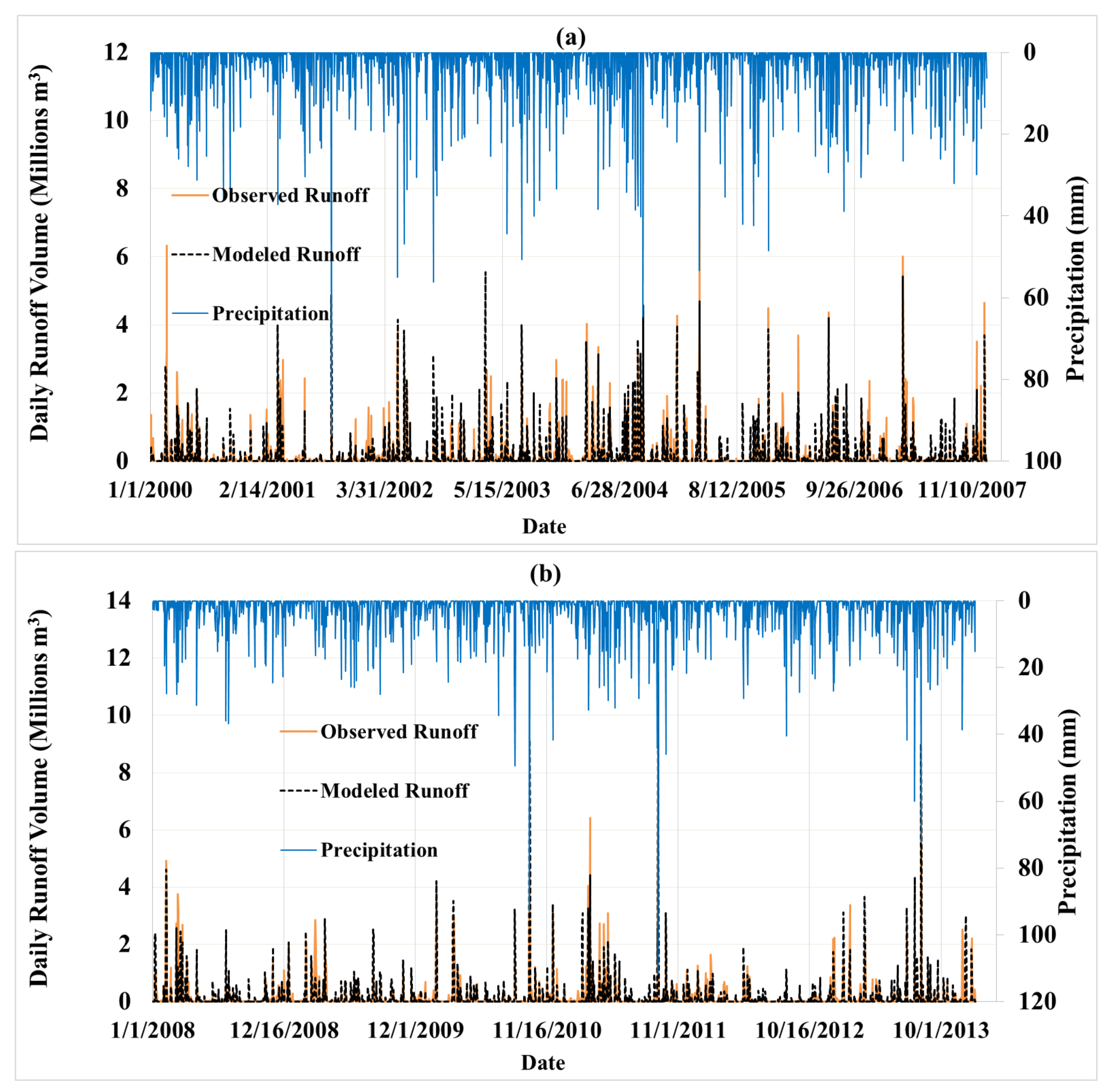
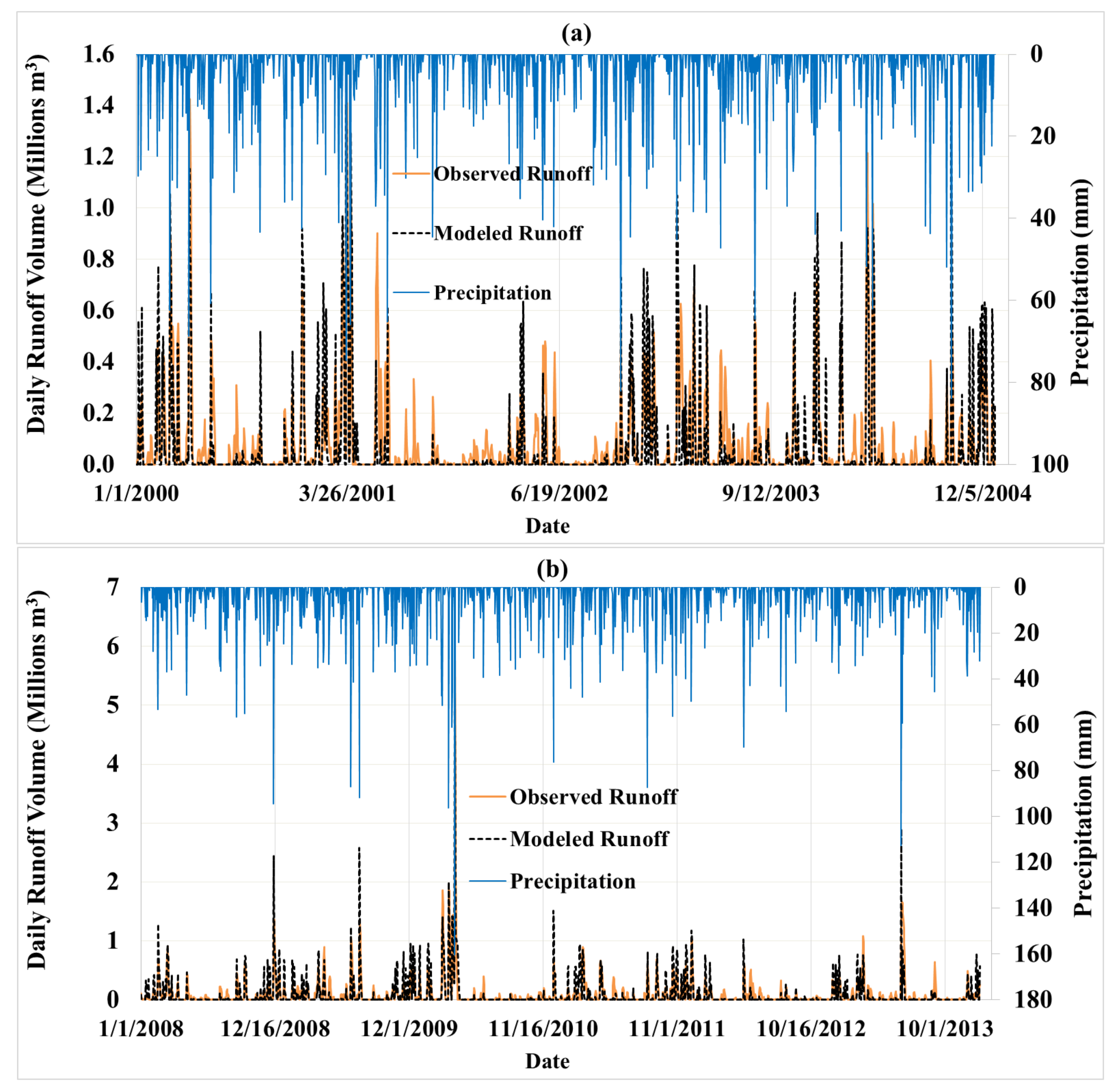
3.1. Runoff Calibration and Validation

According to the classification tabulated in [31] for model correlations and efficiencies modified from [62], our calibrated model for the Sugar Creek watershed predicted the daily runoff volume of the watershed with good correlation and good agreement (R2 = 0.57, NSE = 0.57 for daily and R2 = 0.67, NSE = 0.63 for monthly calibration) between daily observed and daily modeled runoff volume (Table 4, Figure 2a). The calibrated model, when applied to the same watershed for the validation phase, predicted a daily runoff volume with good correlation and good agreement for both daily and monthly scales (R2 = 0.58, NSE = 0.57 for daily and R2 = 0.72, NSE = 0.68 for monthly) (Table 4, Figure 2b). Total runoff estimation by the model during the calibration phase differed from the observed runoff by only about 6.44%, whereas it differed by about 20.5% during validation. The calculated PBIAS value for calibration was less than 10, which indicated an excellent calibration performance rate. The model was biased to overestimate runoff volume during both calibration and validation phases. The observed runoff volumes from January 2000 to December 2013 at the watershed outlet were used for model calibration and validation at daily and monthly scales. The model over-predicted some runoff volumes during the drier months (December to February), whereas it under-predicted some during the wetter months (May to August) (Figure 2).
In the case of Fall Creek watershed, the statistical evaluation of model performance for calibration and validation is presented in Table 5. The value of NSE for both daily and monthly time scales is greater than 0.5, so the model calibration performance can be rated as good. The positive PBIAS indicated the overall underestimation of runoff by the model compared to the observed runoff volume (calibration phase) and the negative PBIAS indicated the overall overestimation of runoff by the model compared to the observed runoff volume (validation phase). Total runoff estimation by the model during the calibration phase differed from the observed runoff by about 16.5%, whereas it differed by about 5.5% during validation. The calculated PBIAS value for validation was less than 10, which pointed to an excellent model performance. Figure 3a,b graphically illustrates observed and modeled daily runoff volume at the USGS 04234000 for calibration and validation phase, respectively, for Fall Creek watershed. The model over-predicted some runoff volumes during the months in which less precipitation occurred (December to March), whereas it under-predicted some during the months in which more precipitation occurred (April to August) (Figure 3). This tendency of the model could be improved by adjusting the evaporation rate associated with the interception of precipitation events.
In the case of Pawcatuck River watershed, graphical comparisons of daily observed and modeled runoff volumes at the USGS 01117500 were presented in Figure 4a,b for the calibration and validation phase, respectively. The statistical evaluation of model performance for calibration and validation is presented in Table 6. The range of NSE (0.51 to 0.54 for daily and 0.68 to 0.83 for monthly) showed a good agreement between daily observed and modeled runoff volume. The positive PBIAS indicates the overall underestimation of runoff by the model compared to the observed runoff volume for both calibration and validation. Total runoff estimation by the model during the calibration phase differed from the observed runoff by about 21.5%, whereas it differed by about 5.8% during validation. The calculated PBIAS value for validation was less than 10, which pointed to an excellent model performance. The results show a general tendency for AnnAGNPS to overestimate spring (March–May) and summer (June–August) runoff volumes compared to observed data for both calibration and validation periods (Figure 4).
The estimated RSR values varied from 0.65 to 0.70 for daily (fair) and 0.41 to 0.63 for monthly (very good to fair) for all three watersheds during calibration and validation periods.

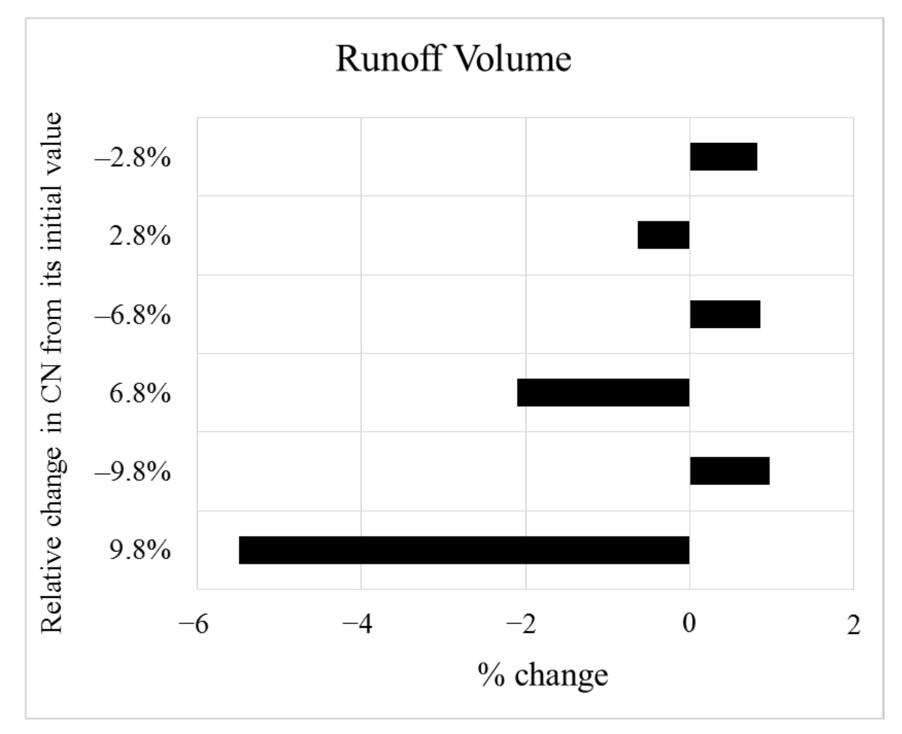
3.2. Sensitivity Analysis

After the sensitivity analysis, it was quite clear how sensitive the CN was for runoff simulation in AnnAGNPS model. The sensitivity analysis demonstrated differences between sites in the response of modeled runoff to changes in CN. In Sugar Creek, the percent change in runoff volume (2000–2007 or 7-year average) from its initial condition was found to be up to 5.5 due to 9.8% changes in the CN (Figure 5).
In the case of Fall Creek watershed, during the entire phase of modification of CN, the percent change in runoff volume (2000–2007 or 7-year average) from its initial condition ranged from 11 to 149 due to 2.6% to 13.6% changes in the CN (Figure 6).
In the case of Pawcatuck River watershed, during the entire phase of modification of CN for Row Crop (SR—Good), the percent change in runoff volume (2000–2004 or 5-year average) from its initial condition ranged from 1.4 to 180 due to −30% to 30% changes in the CN (Figure 7a). The percent change in runoff volume (2000–2004 or 5-year average) from its initial condition ranged from 0.41 to 9.5 due to −10% to 30% changes in the CN for Row Crop (C + CR—Good) (Figure 7b). The percent change in runoff volume (2000–2004 or 5-year average) from its initial condition ranged from 9 to 82 due to −10% to 30% changes in the CN for Woods (Good) (Figure 7c).

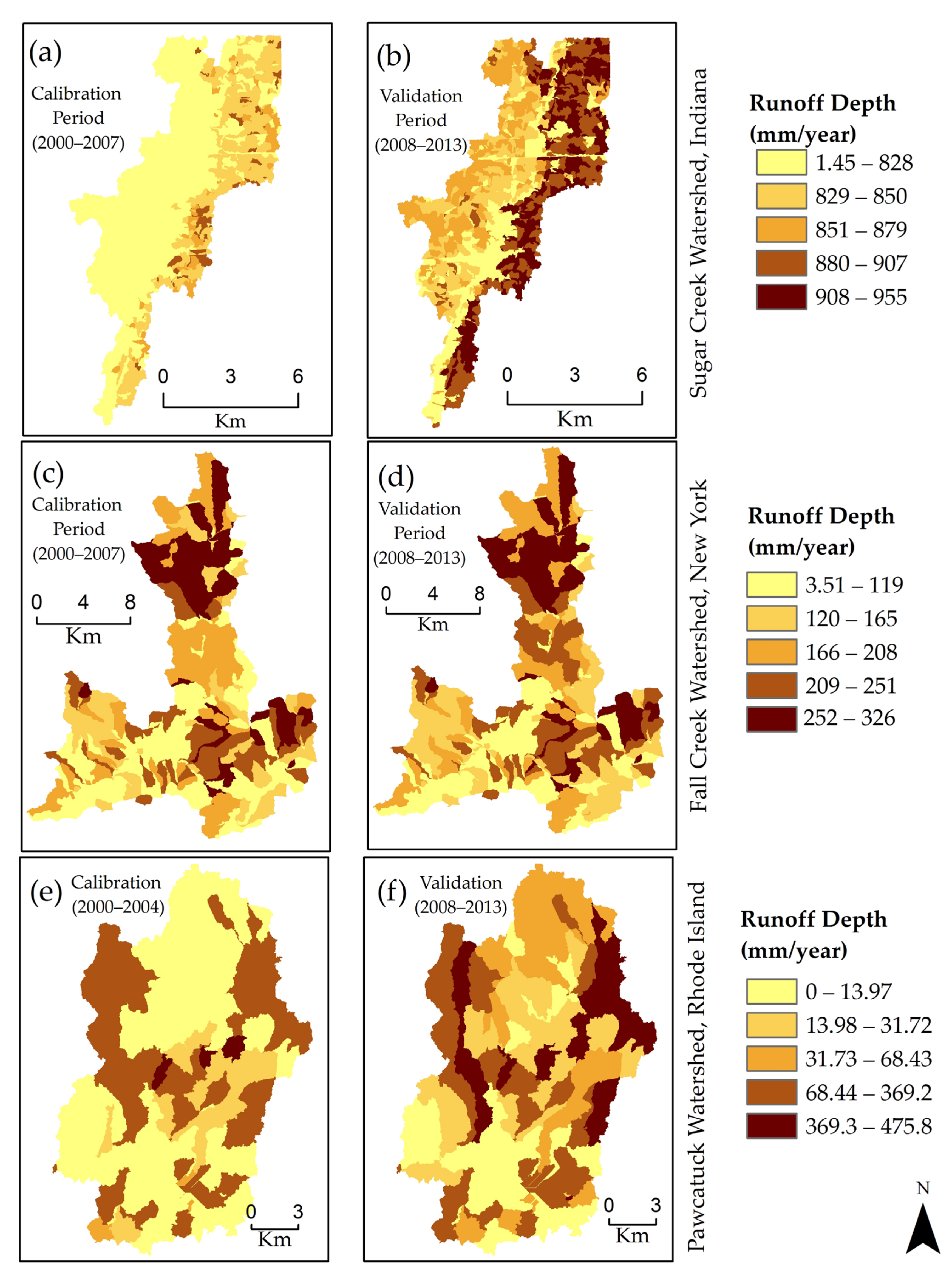
3.3. Spatial Distribution of Runoff Depth

Since the AnnAGNPS model is able to provide landscape spatial variability by representing a watershed with a number of land areas (cells), we also evaluated the average annual runoff depth for all the watersheds (Figure 8). In this figure, the different shades of color indicate different average annual runoff depths in mm/year for each individual cell in a watershed. The darker shades in the figure represent higher runoff depths. At the outlet of the Sugar Creek Watershed, the average annual runoff depth is 755.1 mm and 830.5 mm for calibration period (2000–2007) and validation period (2008–2013), respectively. The runoff depth for each cell (mm/year) for this watershed ranged from 1.45 to 955 mm/year. At the outlet of the Fall Creek Watershed, the average annual runoff depth is 174.0 mm and 185.5 mm for calibration period (2000–2007) and validation period (2008–2013), respectively. The runoff depth for each cell (mm/year) for this watershed ranged from 3.51 to 326 mm/year. At the outlet of the Pawcatuck River Watershed, the average annual runoff depth is 97.1 mm and 135.9 mm for calibration period (2000–2004) and validation period (2008–2013), respectively. The runoff depth for each cell (mm/year) for this watershed ranged from 0.0 to 475.8 mm/year.

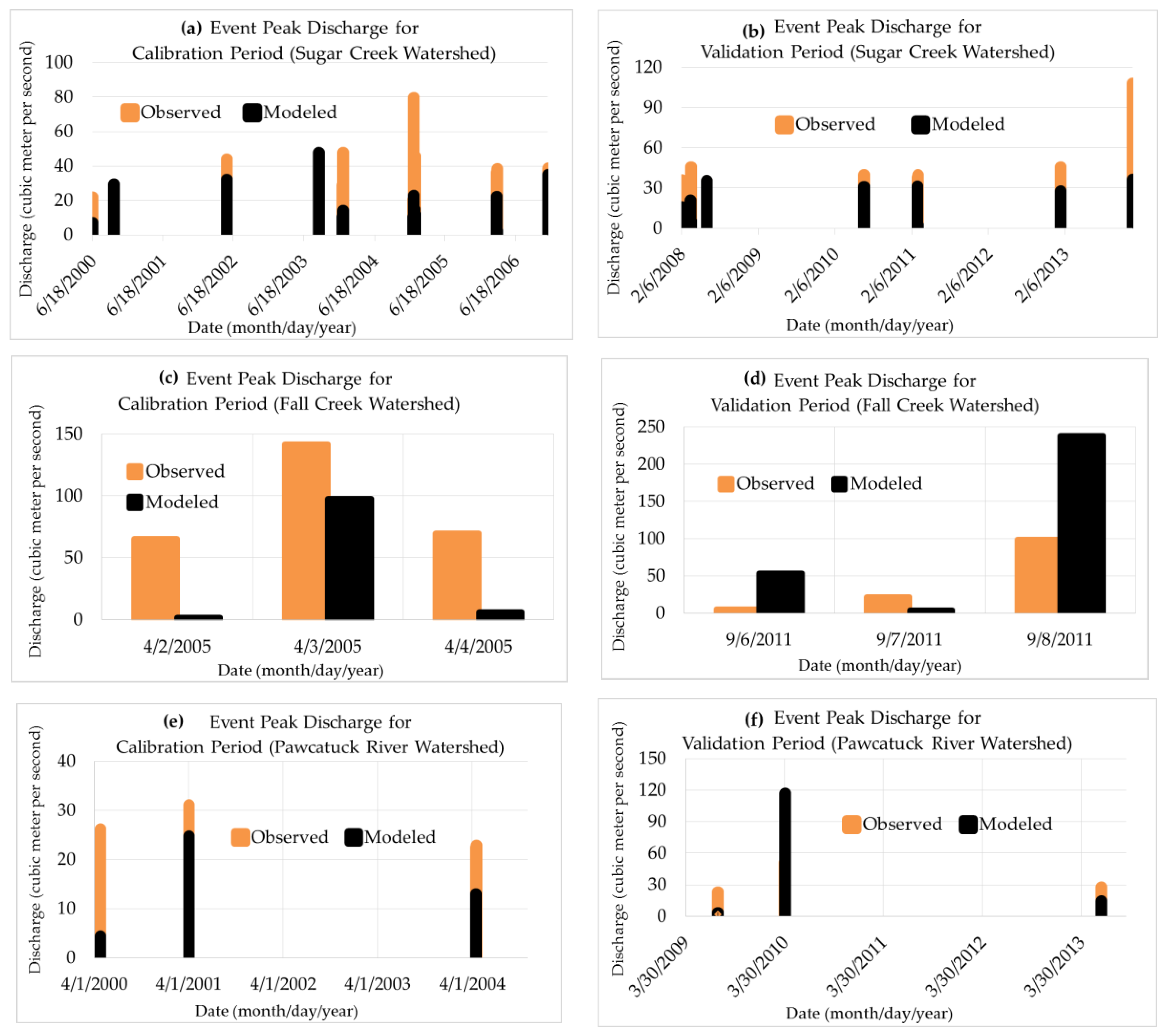
3.4. Model Performance to Estimate Event Peak Discharge

After the successful calibration and validation of runoff volumes, the model performance for the estimation of event peak discharge was done. For this purpose, we first looked at the gage height data for the selected USGS gauging stations. Then, we picked only the events when the gage height exceeded the existing flood stage (determined by USGS) for the particular station. The existing flood stage is 2.4 meters, 1.8 meters and 1.5 meters at USGS 03361650, USGS 04234000 and USGS 01117500, respectively. Figure 9 presents a graphical comparison between observed and model simulated event peak discharge (cubic meter per second) for only those selected events for all three watersheds. The model generally underestimated the peak discharge compared to few overestimations (calibration period) for Sugar Creek Watershed. On the other hand, in the case of Fall Creek Watershed, the model performed well to capture the highest peak discharge from tropical storm Lee in September 2011 based on the entire simulation period (2000–2013). Pawcatuck River Watershed showed a similar model performance. The record peak discharge in Rhode Island from the historic flood in March 2010 was captured by the model.

4. Discussion

AnnAGNPS performed satisfactorily for runoff prediction and simulation. Both daily and monthly calibration and validation statistics (NSE > 0.50 and RSR < 0.70, and PBIAS ± 25% based on [62]) of the developed AnnAGNPS model was satisfactory for runoff simulation for all the watersheds in the study. The model is categorized as satisfactorily performing when the range of the NSE value falls between 0.36 and 0.75 [66].
This study tested the applicability of the AnnAGNPS model on a glaciated landscape, which is why the three chosen watersheds are located in a glacial geomorphic setting. The area of the studied watersheds varied from 69 to 328 km2. After the evaluation of developed model performance, it was learned that the range of NSE varied from 0.51 to 0.57 and 0.60 to 0.83 for daily and monthly scale, respectively. This range is quite similar or even better than the 0.69 to 0.75 (on a monthly scale) found by [34] for a Mediterranean agricultural watershed (2.07 km2) in Spain, 0.73 (on a monthly scale) by AnnAGNPS found by [26] for a 289.3 km2 watershed in Illinois, USA, 0.65 (on a monthly scale) by SWAT and 0.48 to 0.58 (on a monthly scale) by AnnAGNPS found by [36] for a Mediterranean watershed (506 km2) in Southern Italy, 0.53 (on a daily scale) by SWAT found by [67] for a large 1110 km2 agricultural watershed in southwest France, 0.67 to 0.84 (on a monthly scale; calibration phase) found by SWAT for a large 4000 km2 watershed in the North Carolina coastal plain [68], and the 0.53 to 0.62 (on a daily scale) found by SWAT for two watersheds in a semiarid region of Iraq [69]. Even, if we look at the value of R2 from our study, it ranged from 0.54 to 0.66 (daily) and 0.64 to 0.86 (monthly). This range is also better than the one (0.50 to 0.80 by AnnAGNPS and 0.62 to 0.81 by SWAT on a monthly scale) found by [31] for an agricultural watershed in south–central Kansas. We also compared our developed AnnAGNPS model evaluation results with the results found from another water quality model, GLEAMS, in a study by [70] for agricultural watersheds in Indiana. The runoff calibration results were reported by [70] as NSE = 0.62 and R2 = 0.70 for a monthly scale, which is quite similar to our results (NSE = 0.63 and R2 = 0.67 for Sugar Creek; NSE = 0.60 and R2 = 0.64 for Fall Creek; NSE = 0.68 and R2 = 0.75 for Pawcatuck) for our studied watersheds.
Simulated runoff followed a similar trend (seasonal fluctuation) to observed runoff. In general, the model performed better in capturing event peak discharge for Fall Creek and Pawcatuck River watersheds rather than Sugar Creek Watershed. This poor performance of the model at the Sugar Creek Watershed could be improved by testing the effect of different storm types for rainfall distribution. As the regression coefficients for calculating the unit peak discharge are determined by storm type, the storm type within the AnnAGNPS model significantly influences peak discharge [71]. Simulated peak runoff was underestimated during some flood periods such as a major January 2005 flood event, record December 2013 flooding in Sugar Creek watershed, and a major April 2005 flood in Fall Creek watershed. In most cases, the model could not accurately simulate the flood runoff when the river overflowed. This characteristic of a hydrological model such as, AnnAGNPS is similar to that found in studies carried out by other studies (AnnAGNPS and SWAT performed poorly due to several extraordinary floods recorded during the study period in [36]; the SWAT model underestimated the largest flood in the study of [67]). However, the model was able to capture the historic September 2011 flood caused by tropical storm Lee in the case of Fall Creek watershed. In addition to that, the model even successfully captured the peak runoff volume (3815724.36 m3 on 30 March 2010) generated from the historic 2010 flood in Rhode Island during the validation phase. Daily simulated runoff was also overestimated for some periods. Larger errors occurred when simulated peak runoff and average runoff differed significantly from the observed runoff volume. The spatial variability of the runoff depth (Figure 8) could be attributed to the differences in land use, topography, soil type, and soil physical characteristics [58]. The output (spatial variability, i.e., cell wise runoff depth within the watershed) of the AnnAGNPS model contributes the riparian model field input data required for further research.

5. Conclusions

Model performance during calibration and validation phases shows that AnnAGNPS can be successfully used to predict runoff from watersheds in the glaciated settings of the Northeast and Midwest United States. This provides the capacity to couple edge-of-field hydrologic modeling with models that examine riparian or riverine functions and behaviors. The AnnAGNPS model effectively estimated runoff volume and portrayed the seasonal pattern of runoff in all the studied watersheds. The developed AnnAGNPS model could not capture some peak runoff events during wet periods and formed some unnecessary over-prediction of runoff during dry periods of the year. This characteristic of the model could be improved by the readjustment of the evaporation rate in association with the interception of precipitation events. The sensitivity analysis was limited to one specific contributing land use only, which could be extended by considering all possible combinations of CN based on the mixed land use of the watershed.

Author Contributions

M.T. was responsible for the conceptualization, methodology, data processing, software, calibration, validation, formal analysis, writing—original draft preparation, and editing; S.M.P. was responsible for the conceptualization, funding acquisition, methodology, model/software supervision, and writing—review and editing; A.J.G., K.A. and P.G.V. were responsible for the conceptualization, funding acquisition, and writing—review and editing; R.L.B. was responsible for model/software supervision, as well as writing—review and editing. All authors have read and agreed to the published version of the manuscript.

Funding

This study was supported by an Agriculture and Food Research Initiative (AFRI) competitive grant under the United States Department of Agriculture (USDA)—National Institute of Food and Agriculture (NIFA) (grant number 2015-67019-23586).

Acknowledgments

The authors would like to thank Khurshid Jahan, graduate student, Department of Geosciences, University of Rhode Island, for providing support in the processing of PRISM climate data.

Conflicts of Interest

The authors declare no conflict of interest.

References

  1. Diaz, R.J. Overview of hypoxia around the world. J. Environ. Qual. 2001, 30, 275–281. [Google Scholar] [CrossRef] [PubMed]
  2. Driscoll, C.T.; Whitall, D.; Aber, J.; Boyer, E.; Castro, M.; Cronan, C.; Goodale, C.L.; Groffman, P.; Hopkinson, C.; Lambert, K. Nitrogen pollution in the northeastern united states: Sources, effects, and management options. Bioscience 2003, 53, 357–374. [Google Scholar] [CrossRef]
  3. Goolsby, D.A.; Battaglin, W.A.; Aulenbach, B.T.; Hooper, R.P. Nitrogen flux and sources in the Mississippi river basin. Sci. Total Environ. 2000, 248, 75–86. [Google Scholar] [CrossRef] [Green Version]
  4. Howarth, R.W.; Anderson, D.B.; Cloern, J.E.; Elfring, C.; Hopkinson, C.S.; Lapointe, B.; Malone, T.; Marcus, N.; McGlathery, K.; Sharpley, A.N. Nutrient Pollution of Coastal Rivers, Bays, and Seas. Issues in Ecology; Ecological Society of America: Washington, DC, USA, 2000; pp. 1–16. [Google Scholar]
  5. Nixon, S.; Buckley, B.; Granger, S.; Bintz, J. Responses of very shallow marine ecosystems to nutrient enrichment. Human Ecol. Risk Assess. Int. J. 2001, 7, 1457–1481. [Google Scholar] [CrossRef]
  6. Rabalais, N.N.; Turner, R.E.; Wiseman, W.J., Jr. Hypoxia in the Gulf of Mexico. J. Environ. Qual. 2001, 30, 320–329. [Google Scholar] [CrossRef] [PubMed]
  7. David, M.B.; Gentry, L.E. Anthropogenic Inputs of Nitrogen and Phosphorus and Riverine Export for Illinois, USA. J. Environ. Qual. 2000, 29, 494–508. [Google Scholar] [CrossRef]
  8. Martin, T.L.; Kaushik, N.K.; Trevors, J.T.; Whiteley, H.R. Denitrification in temperate climate riparian zones. Water Air Soil Pollut. 1999, 111, 171–186. [Google Scholar] [CrossRef]
  9. Rhode Island Department of Environmental Management (RIDEM). Total Maximum Daily Load Report: The Sakonnet River, Portsmouth Park and The Cove; Rhode Island Department of Environmental Management: Island Park, RI, USA, 2003; Volume 40. [Google Scholar]
  10. Sharpley, A.; Jarvie, H.P.; Buda, A.; May, L.; Spears, B.; Kleinman, P. Phosphorus legacy: Overcoming the effects of past management practices to mitigate future water quality impairment. J. Environ. Qual. 2013, 42, 1308–1326. [Google Scholar] [CrossRef] [Green Version]
  11. Dosskey, M.G. Toward quantifying water pollution abatement in response to installing buffers on crop land. Environ. Manag. 2001, 28, 577–598. [Google Scholar] [CrossRef]
  12. Welsch, D.J. Riparian Forest Buffers: Function and Design for Protection and Enhancement of Water Resources; US Department of Agriculture, Forest Service, Northeastern Area, State & Private Forestry, Forest Resources Management: Washington, DC, USA, 1991; Volume 7.
  13. Gold, A.J.; Groffman, P.M.; Addy, K.; Kellogg, D.Q.; Stolt, M.; Rosenblatt, A.E. Landscape attributes as controls on ground water nitrate removal capacity of riparian zones 1. JAWRA J. Am. Water Resour. Assoc. 2001, 37, 1457–1464. [Google Scholar] [CrossRef]
  14. Hill, A.R. Stream chemistry and riparian zones. In Streams Ground Waters; Elsevier: Amsterdam, The Netherlands, 2000; pp. 83–110. [Google Scholar]
  15. Inamdar, S.P.; Sheridan, J.M.; Williams, R.G.; Bosch, D.D.; Lowrance, R.R.; Altier, L.S.; Thomas, D.L. Riparian ecosystem management model (REMM): I. Testing of the hydrologic component for a coastal plain riparian system. Trans. ASAE 1999, 42, 1679. [Google Scholar] [CrossRef]
  16. Kellogg, D.Q.; Gold, A.J.; Groffman, P.M.; Addy, K.; Stolt, M.H.; Blazejewski, G. In situ ground water denitrification in stratified, permeable soils underlying riparian wetlands. J. Environ. Qual. 2005, 34, 524–533. [Google Scholar] [CrossRef] [PubMed]
  17. Lowrance, R.; Vellidis, G.; Wauchope, R.D.; Gay, P.; Bosch, D.D. Herbicide transport in a managed riparian forest buffer system. Trans. ASAE 1997, 40, 1047–1057. [Google Scholar] [CrossRef]
  18. Peterjohn, W.T.; Correll, D.L. Nutrient dynamics in an agricultural watershed: Observations on the role of a riparian forest. Ecology 1984, 65, 1466–1475. [Google Scholar] [CrossRef]
  19. Vidon, P.; Hill, A.R. Denitrification and patterns of electron donors and acceptors in eight riparian zones with contrasting hydrogeology. Biogeochemistry 2004, 71, 259–283. [Google Scholar] [CrossRef]
  20. Vidon, P.; Smith, A.P. Upland Controls on the Hydrological Functioning of Riparian Zones in Glacial Till Valleys of the Midwest 1. JAWRA J. Am. Water Resour. Assoc. 2007, 43, 1524–1539. [Google Scholar] [CrossRef]
  21. Altier, L.S.; Lowrance, R.; Williams, R.G.; Inamdar, S.P.; Bosch, D.D.; Sheridan, J.M.; Hubbard, R.K.; Thomas, D.L. Riparian Ecosystem Management Model: Simulator for Ecological Processes in Riparian Zones; Conservation Research Report 46; United States Department of Agriculture: Washington, DC, USA, 2002; Volume 46, p. 216.
  22. Lowrance, R.; Altier, L.S.; Williams, R.G.; Inamdar, S.P.; Sheridan, J.M.; Bosch, D.D.; Hubbard, R.K.; Thomas, D.L. REMM: The riparian ecosystem management model. J. Soil Water Conserv. 2000, 55, 27–34. [Google Scholar]
  23. Sopper, W.E.; Lull, H.W. Streamflow characteristics of physiographic units in the northeast. Water Resour. Res. 1965, 1, 115–124. [Google Scholar] [CrossRef]
  24. Bingner, R.L.; Theurer, F.D. AnnAGNPS: Estimating Sediment Yield by Particle Size for Sheet and Rill Erosion. In Proceedings of the 7th Interagency Sedimentation Conference, Reno, NV, USA, 25–29 March 2001. [Google Scholar]
  25. Geter, W.F.; Theurer, F.D. AnnAGNPS-RUSLE sheet and rill erosion. In Proceedings of the First Federal Interagency Hydrologic Modeling Conference, Las Vegas, NV, USA, 19–23 April 1998. [Google Scholar]
  26. Yuan, Y.; Mehaffey, M.H.; Lopez, R.D.; Bingner, R.L.; Bruins, R.; Erickson, C.; Jackson, M.A. AnnAGNPS model application for nitrogen loading assessment for the future Midwest landscape study. Water 2011, 3, 196–216. [Google Scholar] [CrossRef] [Green Version]
  27. Zuercher, B.W.; Flanagan, D.C.; Heathman, G.C. Evaluation of the AnnAGNPS model for atrazine prediction in northeast Indiana. Trans. ASABE 2011, 54, 811–825. [Google Scholar] [CrossRef]
  28. Karki, R.; Tagert, M.L.M.; Paz, J.O.; Bingner, R.L. Application of AnnAGNPS to model an agricultural watershed in east-central mississippi for the evaluation of an on-farm water storage (OFWS) system. Agric. Water Manag. 2017, 192, 103–114. [Google Scholar] [CrossRef]
  29. Yasarer, L.M.; Bingner, R.L.; Momm, H.G. Characterizing ponds in a watershed simulation and evaluating their influence on streamflow in a Mississippi watershed. Hydrol. Sci. J. 2018, 63, 302–311. [Google Scholar] [CrossRef]
  30. Suttles, J.B.; Vellidis, G.; Bosch, D.D.; Lowrance, R.; Sheridan, J.M.; Usery, E.L. Watershed–scale simulation of sediment andnutrient loads in Georgia coastal plain streams using the annualized AGNPS model. Trans. ASAE 2003, 46, 1325. [Google Scholar] [CrossRef] [Green Version]
  31. Parajuli, P.B.; Nelson, N.O.; Frees, L.D.; Mankin, K.R. Comparison of AnnAGNPS and SWAT model simulation results in USDA-CEAP agricultural watersheds in south-central Kansas. Hydrol. Process. Int. J. 2009, 23, 748–763. [Google Scholar] [CrossRef]
  32. Pradhanang, S.M. Monitoring and Modeling of Water Quality in Streams of Skaneateles Lake Watershed, NY; State University of New York College of Environmental Science and Forestry: Syracuse, NY, USA, 2010. [Google Scholar]
  33. Zema, D.A.; Lucas-Borja, M.E.; Carrà, B.G.; Denisi, P.; Rodrigues, V.A.; Ranzini, M.; Arcova, F.C.S.; de Cicco, V.; Zimbone, S.M. Simulating the hydrological response of a small tropical forest watershed (Mata Atlantica, Brazil) by the AnnAGNPS model. Sci. Total Environ. 2018, 636, 737–750. [Google Scholar] [CrossRef] [PubMed] [Green Version]
  34. Chahor, Y.; Casalí, J.; Giménez, R.; Bingner, R.L.; Campo, M.A.; Goñi, M. Evaluation of the AnnAGNPS model for predicting runoff and sediment yield in a small Mediterranean agricultural watershed in navarre (Spain). Agric. Water Manag. 2014, 134, 24–37. [Google Scholar] [CrossRef]
  35. Ogwo, V. Streamflow and Sediment Yield Prediction using AnnAGNPS Model in Upper Ebonyi River Watershed, South-Eastern Nigeria. Agric. Eng. Int. CIGR J. 2019, 20, 50–62. [Google Scholar]
  36. Abdelwahab, O.; Ricci, G.F.; de Girolamo, A.M.; Gentile, F. Modelling soil erosion in a mediterranean watershed: Comparison between SWAT and AnnAGNPS models. Environ. Res. 2018, 166, 363–376. [Google Scholar] [CrossRef]
  37. Abdelwahab, O.M.M.; Bingner, R.L.; Milillo, F.; Gentile, F. Evaluation of alternative management practices with the AnnAGNPS model in the Carapelle watershed. Soil Sci. 2016, 181, 293–305. [Google Scholar] [CrossRef]
  38. Licciardello, F.; Zema, D.A.; Zimbone, S.M.; Bingner, R.L. runoff and soil erosion evaluation by the AnnAGNPS model in a small mediterranean watershed. Trans. ASABE 2007, 50, 1585–1593. [Google Scholar] [CrossRef]
  39. Das, S.; Rudra, R.P.; Gharabaghi, B.; Gebremeskel, S.; Goel, P.K.; Dickinson, W.T. Applicability of AnnAGNPS for Ontario conditions. Can. Biosyst. Eng. 2008, 50, 1–11. [Google Scholar]
  40. Baginska, B.; Milne-Home, W.; Cornish, P.S. Modelling nutrient transport in currency creek, NSW with AnnAGNPS and PEST. Environ. Model. Softw. 2003, 18, 801–808. [Google Scholar] [CrossRef]
  41. Shrestha, S.; Babel, M.S.; Gupta, A.D.; Kazama, F. Evaluation of annualized agricultural nonpoint source model for a watershed in the Siwalik Hills of Nepal. Environ. Model. Softw. 2006, 21, 961–975. [Google Scholar] [CrossRef]
  42. Li, Z.; Luo, C.; Xi, Q.; Li, H.; Pan, J.; Zhou, Q.; Xiong, Z. Assessment of the AnnAGNPS model in simulating runoff and nutrients in a typical small watershed in the Taihu Lake basin, China. Catena 2015, 133, 349–361. [Google Scholar] [CrossRef]
  43. Zema, D.A.; Bingner, R.L.; Denisi, P.; Govers, G.; Licciardello, F.; Zimbone, S.M. Evaluation of runoff, peak flow and sediment yield for events simulated by the AnnAGNPS model in a Belgian agricultural watershed. Land Degrad. Dev. 2012, 23, 205–215. [Google Scholar] [CrossRef]
  44. Shamshad, A.; Leow, C.S.; Ramlah, A.; Hussin, W.W.; Sanusi, S.M. Applications of AnnAGNPS model for soil loss estimation and nutrient loading for Malaysian conditions. Int. J. Appl. Earth Obs. Geoinf. 2008, 10, 239–252. [Google Scholar] [CrossRef]
  45. Sarangi, A.; Cox, C.A.; Madramootoo, C.A. Evaluation of the AnnAGNPS model for prediction of runoff and sediment yields in St Lucia watersheds. Biosyst. Eng. 2007, 97, 241–256. [Google Scholar] [CrossRef]
  46. Vidon, P.; Cuadra, P.E. Impact of precipitation characteristics on soil hydrology in tile-drained landscapes. Hydrol. Process. 2010, 24, 1821–1833. [Google Scholar] [CrossRef]
  47. Lathrop, T.R. Environmental Setting of the Sugar Creek and Leary Weber Ditch Basins, Indiana, 2002-04; National Water-Quality Assessment Program: Yantai, China, 2006.
  48. Fenelon, J.M.; Moore, R.C. Transport of agrichemicals to ground and surface water in a small central Indiana watershed. J. Environ. Qual. 1998, 27, 884–894. [Google Scholar] [CrossRef]
  49. Johnson, M.S.; Woodbury, P.B.; Pell, A.N.; Lehmann, J. Land-use change and stream water fluxes: Decadal dynamics in watershed nitrate exports. Ecosystems 2007, 10, 1182–1196. [Google Scholar] [CrossRef]
  50. Dikshit, A.K.; Loucks, D.P. Estimating Non-Point Pollutant Loadings-II: A Case Study in the Fall Creek Watershed, New York. J. Environ. Syst. 1996, 25, 81. [Google Scholar] [CrossRef]
  51. Rook, S.P. Riparian Zone Hydrology and Biogeochemistry as a Function of Stream Evolution Stage in a Glaciated Landscape of the US Northeast; State University of New York College of Environmental Science and Forestry: Syracuse, NY, USA, 2012. [Google Scholar]
  52. Rosenblatt, A.E.; Gold, A.J.; Stolt, M.H.; Groffman, P.M.; Kellogg, D.Q. Identifying riparian sinks for watershed nitrate using soil surveys. J. Environ. Qual. 2001, 30, 1596–1604. [Google Scholar] [CrossRef] [PubMed]
  53. Young, R.A.; Onstad, C.A.; Bosch, D.D.; Anderson, W.P. AGNPS: A nonpoint-source pollution model for evaluating agricultural watersheds. J. Soil Water Conserv. 1989, 44, 168–173. [Google Scholar]
  54. Renard, K.G. Predicting Soil Erosion by Water: A Guide to Conservation Planning with the Revised Universal Soil Loss Equation (RUSLE); United States Government Printing: Washington, DC, USA, 1997.
  55. Knisel, W.G. CREAMS: A Field Scale Model for Chemicals, Runoff, and Erosion from Agricultural Management Systems; Department of Agriculture, Science and Education Administration: Corvallis, OR, USA, 1980. [Google Scholar]
  56. Sharpley, A.N.; Williams, J.R. EPIC-erosion/productivity impact calculator. I: Model documentation. II: User manual. Tech. Bull. United States Dep. Agric 1990, 1768, 1–377. [Google Scholar]
  57. Leonard, R.A.; Knisel, W.G.; Still, D.A. GLEAMS: Groundwater loading effects of agricultural management systems. Trans. ASAE 1987, 30, 1403–1418. [Google Scholar] [CrossRef]
  58. Bingner, R.L.; Theurer, F.; Yuan, Y. AnnAGNPS Technical Processes, Version 5.4; United States Environmental Protection Agency: Washington, DC, USA, 2015. Available online: https://www.wcc.nrcs.usda.gov/ftpref/wntsc/H&H/AGNPS/downloads/AnnAGNPS_Technical_Documentation.pdf (accessed on 1 February 2018).
  59. USDA, S. National Engineering Handbook; Hydrology Section 4; US Department of Agriculture, Soil Conservation Service: Washington, DC, USA, 1972; Chapters 4–10.
  60. Saha, S.; Moorthi, S.; Wu, X.; Wang, J.; Nadiga, S.; Tripp, P.; Behringer, D.; Hou, Y.; Chuang, H.; Iredell, M. The NCEP climate forecast system version 2. J. Clim. 2014, 27, 2185–2208. [Google Scholar] [CrossRef]
  61. Pradhanang, S.M.; Briggs, R.D. Effects of critical source area on sediment yield and streamflow. Water Environ. J. 2014, 28, 222–232. [Google Scholar] [CrossRef]
  62. Moriasi, D.N.; Arnold, J.G.; van Liew, M.W.; Bingner, R.L.; Harmel, R.D.; Veith, T.L. Model evaluation guidelines for systematic quantification of accuracy in watershed simulations. Trans. ASABE 2007, 50, 885–900. [Google Scholar] [CrossRef]
  63. Nash, J.E.; Sutcliffe, J.V. River flow forecasting through conceptual models. Part I—A discussion of principles. J. Hydrol. 1970, 10, 282–290. [Google Scholar] [CrossRef]
  64. Morris, M.D. Factorial sampling plans for preliminary computational experiments. Technometrics 1991, 33, 161–174. [Google Scholar] [CrossRef]
  65. Cronshey, R.G.; Roberts, R.T.; Miller, N. Urban hydrology for small watersheds (TR-55 Rev.). In Hydraulics and Hydrology in the Small Computer Age; American Society of Civil Engineers: Reston, VA, USA, 1986; pp. 1268–1273. [Google Scholar]
  66. van Liew, M.W.; Arnold, J.G.; Garbrecht, J.D. Hydrologic simulation on agricultural watersheds: Choosing between two models. Trans. ASAE 2003, 46, 1539. [Google Scholar] [CrossRef]
  67. Oeurng, C.; Sauvage, S.; Sánchez-Pérez, J. Assessment of hydrology, sediment and particulate organic carbon yield in a large agricultural catchment using the SWAT model. J. Hydrol. 2011, 401, 145–153. [Google Scholar] [CrossRef] [Green Version]
  68. Mapes, K.L.; Pricope, N.G. Evaluating SWAT model performance for runoff, percolation, and sediment loss estimation in low-gradient watersheds of the Atlantic coastal plain. Hydrology 2020, 7, 21. [Google Scholar] [CrossRef] [Green Version]
  69. Al-Khafaji, M.S.; Al-Chalabi, R.D. Assessment and mitigation of streamflow and sediment yield under climate change conditions in Diyala River Basin, Iraq. Hydrology 2019, 6, 63. [Google Scholar] [CrossRef] [Green Version]
  70. Adeuya, R.M.; Lim, K.J.; Engel, B.A.; Thomas, M.A. Modeling the average annual nutrient losses of two watersheds in Indiana using GLEAMS-NAPRA. Trans. ASAE 2005, 48, 1739–1749. [Google Scholar] [CrossRef]
  71. Bisantino, T.; Bingner, R.; Chouaib, W.; Gentile, F.; Trisorio-Liuzzi, G. Estimation of runoff, peak discharge and sediment load at the event scale in a medium-size Mediterranean watershed using the AnnAGNPS model. Land Degrad. Dev. 2015, 26, 340–355. [Google Scholar] [CrossRef]
Figure 1. Three Study Watersheds.
Water 12 03525 g001
Figure 2. Graphical comparison between daily modeled and observed runoff (a) after calibration and (b) validation phase for Sugar Creek Watershed.
Water 12 03525 g002
Figure 3. Graphical comparison between daily modeled and observed runoff after (a) after calibration and (b) validation phase for Fall Creek Watershed.
Water 12 03525 g003
Figure 4. Graphical comparison between daily modeled and observed runoff (a) after calibration and (b) validation phase for Pawcatuck River Watershed.
Water 12 03525 g004
Figure 5. Sensitivity analysis for CN for a straight row crop with poor hydrological conditions; Sugar Creek watershed.
Water 12 03525 g005
Figure 6. Sensitivity analysis for CN for a contoured row crop with poor hydrological conditions; Fall Creek watershed.
Water 12 03525 g006
Figure 7. Sensitivity analysis for (a) CN for Row Crop (SR—Good), (b) CN for Row Crop (C + CR—Good), (c) CN for Woods (Good), Pawcatuck River Watershed.
Water 12 03525 g007
Figure 8. Spatial distribution of average annual runoff depth in mm/year for: (a) calibration period, Sugar Creek Watershed; (b) validation period, Sugar Creek Watershed; (c) calibration period, Fall Creek Watershed; (d) validation period, Fall Creek Watershed; (e) calibration period, Pawcatuck River Watershed; (f) validation period, Pawcatuck River Watershed.
Water 12 03525 g008
Figure 9. AnnAGNPS model estimation of event peak discharge (cubic meter per second) for: (a) calibration period, Sugar Creek Watershed; (b) validation period, Sugar Creek Watershed; (c) calibration period, Fall Creek Watershed; (d) validation period, Fall Creek Watershed; (e) calibration period, Pawcatuck River Watershed; (f) validation period, Pawcatuck River Watershed.
Water 12 03525 g009
Table 1. Curve numbers (CN) used for model calibration, Sugar Creek watershed.
Cover DescriptionCurve Number for Hydrological Soil Groups
Initial ValuesValues After Calibration
ABCDABCD
Row Crop (SR—Poor)7281889174.0283.2790.4693.55
Fallow (CR—Good)74838890Not changed
Woods (Good)30557077Not changed
Urban (85% imp)89929495Not changed
SR—straight row, CR—crop residue cover.
Table 2. Curve Numbers (CN) used for model calibration, Fall Creek watershed.
Cover DescriptionCurve Number for Hydrological Soil Groups
Initial ValuesValues After Calibration
ABCDABCD
Row Crop (SR—Poor)72818891Not changed
Urban (Newly graded)77869194Not changed
Woods—Grass (Poor)57738286Not changed
Fallow (CR—Poor)76859093Not changed
Row Crop (C—Poor)7079848874.6284.2189.5493.81
SR—straight row, CR—crop residue cover, C—contoured.
Table 3. Curve Numbers (CN) used for model calibration, Pawcatuck River watershed.
Cover DescriptionCurve Number for Hydrological Soil Groups
Initial ValuesValues After Calibration
ABCDABCD
Row Crop (SR—Good)6778858935.845.750.562.3
Row Crop (C + CR—Good)6474818558.136874.0578.98
Urban (85% imp)89929495Not changed
Woods (Good)3055707731.549.566.575
SR—straight row, CR—crop residue cover, C—contoured.
Table 4. Runoff calibration and validation results for Sugar Creek watershed.
ParameterCalibration Period
(1 January 2000 to 31 December 2007)
Validation Period
(1 January 2008 to 31 December 2013)
DailyMonthlyDailyMonthly
R20.570.670.580.72
NSE0.570.630.570.68
PBIAS−6.44%−6.47%−20.56%−20.36%
RSR0.660.610.650.57
Table 5. Runoff calibration and validation results for Fall Creek watershed.
ParameterCalibration Period
(1 January 2000 to 31 December 2007)
Validation Period
(1 January 2008 to 31 December 2013)
DailyMonthlyDailyMonthly
R20.540.640.660.66
NSE0.510.600.520.64
PBIAS16.48%16.59%−5.50%−5.51%
RSR0.700.630.690.60
Table 6. Runoff calibration and validation results for Pawcatuck River watershed.
ParameterCalibration Period
(1 January 2000 to 31 December 2004)
Validation Period
(1 January 2008 to 31 December 2013)
DailyMonthlyDailyMonthly
R20.620.750.630.86
NSE0.510.680.540.83
PBIAS21.56%21.15%5.81%5.79%
RSR0.700.560.680.41
Publisher’s Note: MDPI stays neutral with regard to jurisdictional claims in published maps and institutional affiliations.

