Article

Impact of Input Filtering and Architecture Selection Strategies on GRU Runoff Forecasting: A Case Study in the Wei River Basin, Shaanxi, China

College of Water Sciences, Beijing Normal University, Beijing 100875, China
*
Author to whom correspondence should be addressed.
Water 2020, 12(12), 3532; https://doi.org/10.3390/w12123532
Submission received: 21 November 2020 / Revised: 15 December 2020 / Accepted: 15 December 2020 / Published: 16 December 2020
(This article belongs to the Special Issue Advanced Hydrologic Modeling in Watershed-Scale)

Abstract

:
A gated recurrent unit (GRU) network, which is a kind of artificial neural network (ANN), has been increasingly applied to runoff forecasting. However, knowledge about the impact of different input data filtering strategies and the implications of different architectures on the GRU runoff forecasting model’s performance is still insufficient. This study has selected the daily rainfall and runoff data from 2007 to 2014 in the Wei River basin in Shaanxi, China, and assessed six different scenarios to explore the patterns of that impact. In the scenarios, four manually-selected rainfall or runoff data combinations and principal component analysis (PCA) denoised input have been considered along with single directional and bi-directional GRU network architectures. The performance has been evaluated from the aspect of robustness to 48 various hypermeter combinations, also, optimized accuracy in one-day-ahead (T + 1) and two-day-ahead (T + 2) forecasting for the overall forecasting process and the flood peak forecasts. The results suggest that the rainfall data can enhance the robustness of the model, especially in T + 2 forecasting. Additionally, it slightly introduces noise and affects the optimized prediction accuracy in T + 1 forecasting, but significantly improves the accuracy in T + 2 forecasting. Though with relevance (R = 0.409~0.763, Grey correlation grade >0.99), the runoff data at the adjacent tributary has an adverse effect on the robustness, but can enhance the accuracy of the flood peak forecasts with a short lead time. The models with PCA denoised input has an equivalent, even better performance on the robustness and accuracy compared with the models with the well manually filtered data; though slightly reduces the time-step robustness, the bi-directional architecture can enhance the prediction accuracy. All the scenarios provide acceptable forecasting results (NSE of 0.927~0.951 for T + 1 forecasting and 0.745~0.836 for T + 2 forecasting) when the hyperparameters have already been optimized. Based on the results, recommendations have been provided for the construction of the GRU runoff forecasting model.

1. Introduction

Runoff forecasting plays an essential role in flood mitigation management, agricultural water management, water transportations, and other socio-economical activities closely related to water resources. Many approaches, including physics-based models [1,2,3] and data-driven models [4,5,6], have been developed during recent decades to obtain a precise prediction result of the runoff.
Some physics-based hydrological models, such as SWAT [7,8,9], TOPMODEL/BTOP-MC [10,11], and MIKE SHE [12,13], have already been widely used to simulate the rainfall-runoff relationship for runoff prediction because of the definite and explainable mechanisms and the theoretically high accuracy of the modelling results, in addition to the user-friendly interfaces of the modelling software. However, the above-mentioned physics-based models usually require the observed rainfall as the input and the observed runoff data for calibration/validation and some additional data, like the digital elevation model (DEM), soil types, and land use information. The modelling results usually show the different extent of dependencies on the presence, appropriateness, and the resolution of those additional data [14]. This dependency might restrain the practical implementation of the models.
Contrary to the hydrological/hydrodynamic models that are mainly based upon a series of definite physical mechanisms, the data-driven models only consider the statistical relationship of the data [15]. Machine learning is one of the most commonly utilized approaches for exploring the numeric connections between the input and the target data. Several kinds of machine learning model that can be used to attain a precise estimation on the short-term runoff have been shown in several pieces of research. For example, the support vector machine [16,17,18] and the random forest regressor [19,20]. As a subset of machine learning, deep learning, which is mainly represented by the artificial neural network (ANN) techniques, is of great interest nowadays due to the booming computer science and algorithms [21]. Since its ability to seek out the complicated nonlinear relationships between the given datasets, the ANNs can be applied to complex systems’ modeling tasks. In the hydrological field, the ANNs have been used for different aims, for instance, flood or runoff forecasting [17,22,23,24], rainfall forecasting [25,26,27], and evapotranspiration prediction [28,29].
The ANNs can also be categorized into several subdivisions according to their specific structures; in other words, their characteristics. The designs of the ANNs result in the diversity of their advancements and limitations [30]. For example, the convolutional neural networks have the kernel to recognize the spatial distribution pattern of data; consequently, it has been implemented commonly for imagery classification [31,32,33], however, the existence of pooling layers may cause the loss of abundant information [34]. The recurrent neural network (RNN) is a “loop” structure that has a state to store the information from the previous steps; thus, it can deal with the time-series data that has time dependency. Despite the advancement of the RNNs from the aspect of time series processing, when dealing with the long-term dependency sequences, the performance of the conventional RNN cells is not satisfactory enough as a result of the vanishing or exploding gradients. Long short-term memory (LSTM) networks, a variant of RNNs [35], solved the drawbacks of the traditional RNNs. There has been plenty of research in various realms that utilized the LSTM networks to process the time series data successfully, for instance, natural language processing (NLP) [36,37,38], water or air quality forecasting [39,40,41], and disease diagnoses [42,43]. The LSTM network also has some variants; one is the gated recurrent unit (GRU) network [44], which needs fewer calculations than an LSTM cell. As a result, the GRU networks usually show a higher training efficiency than the LSTM networks [45,46].
For the runoff forecasting, the runoff has an apparent long-term dependency on the rainfall data [47] and the reliance on the previous upstream runoff data; the characteristics of LSTM/GRU are appropriate for this type of assignment. Several studies have shown that the LTSM networks or GRU networks can obtain impressive results when carrying out runoff or flood forecasting assignments. The LSTM network has been implemented in the Da River basin in Vietnam for one-day, two-day, and three-day ahead flowrate forecasting cases and got the Nash–Sutcliffe efficiency (NSE) of 99%, 95%, and 87% correspondingly for each case [15]. A flood forecasting model with a spatiotemporal attention mechanism based on LSTM has been used in Lech and Changhua river basins and obtained a lower root mean square error (RMSE), a lower mean absolute percent error (MAPE), and a higher deterministic coefficient (DC) compared with SVM and fully-connected network (FCN) for six- and nine-time step flood predictions [48]. A self-attentive long short-term memory (SA-LSTM) network has been evaluated at eight runoff datasets for 1~7 days ahead forecasting. It has been shown to have the best prediction accuracy in several models [49]. A deep neural network called CAGANet, which consists of a convolutional layer, an attention mechanism, a GRU neural network, and an autoregressive (AR) model, has been proposed for daily runoff predictions in Qingxi river basin, Sichuan Province, China, the NSE reached 0.993 [50]. Despite the good performances of LSTM networks and GRU networks in recent studies, most of them focus on improving the optimized prediction accuracy by modifying or coupling the models. There have been few attempts to demonstrate the impact of different input datasets, as well as the model’s structure on the performance of the model, especially in the model construction stage. Though not mainly focusing on this problem, some researchers have preliminarily revealed that input filtering has an impact on the forecasting model. For instance, relevant research [15] suggests that a higher correlation coefficient between the input and the target datasets can better the forecasting model’s performance. Meanwhile, the inclusion of the rainfall data might not significantly enhance the prediction accuracy and sometimes even negatively impact it. Another study [51] shows that a better prediction result (the test NSE of 0.942 compared with 0.666) has been obtained when using a selected subset of all rain gauges as the input. Furthermore, the LSTM or GRU networks’ architectures can also influence the forecasting results [52,53].
The problem is that although these studies have shown the impact of the input and the networks’ structure on the final performance, this impact still needs to be adequately evaluated. It should be carefully considered at the stage of preprocessing and model construction.
In this research, to comprehensively explore the specific impact of the different input filtering strategies, in addition to the effects of the networks’ architectures on the GRU-based runoff forecasting model, we constructed several models that use the flowrate (at hydrological stations) and the rainfall data (at meteorological stations) as the input. The Wei River basin, which is a typical region with a continental climate and distinct seasons [54], located in Shaanxi, China, is selected as the study area. Four scenarios of the input dataset with different combinations of the hydrological stations and the meteorological stations, two principal component analysis (PCA) denoising based scenarios with single- and bi-directional architectures for one-day-ahead and two-day-ahead predictions have been conducted. A scope of hyperparameters, including the number of hidden units, the number of hidden layers, and the length of the input time steps, has been set to make the comparison. The models have been evaluated from the aspect of robustness [55] to hyperparameters and accuracy. The knowledge about the particular impact of the input and architectures on the performance of the model can be valuable in the model construction stage since it can act as guidance and help to construct a more robust and accurate forecasting model within a more convenient process. Recommendations based on that knowledge could be a good reference for future studies and practical applications.

2. Methodology

2.1. Preprocessing

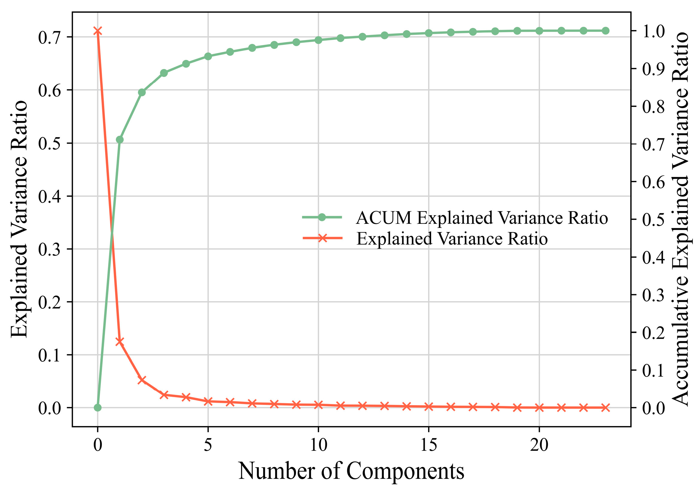
2.1.1. Principal Component Analysis (PCA) Denoising

The PCA method is utilized in the preprocessing stage in two of the scenarios (refer to the scenarios setting situation in Section 3.2) for column vector selection. Typically, it is used as an unsupervised algorithm to delete the redundant components in the input dataset and only maintain the components that explain most of the variance. Through the PCA operation, the initial N-dimensional matrix will be transformed into a K-dimensional matrix (K < N). The calculation processes in the PCA component reduction operation can refer to the following literature [56,57,58].
After the component reduction process in the PCA operation, the processed matrix is then re-projected to form a matrix that has the same dimension (or the same shape) as the initial input matrix. What should be mentioned is that the filtered information will not be included in the re-projection process.

2.1.2. Normalization

For the scenarios without PCA denoising operation, the rainfall and runoff data is normalized with Equation (1), called Min-Max normalization. The normalized data has a value range of [1]:
x = x min ( x ) max ( x ) min ( x )
where x is the normalized data, min ( x ) and max ( x ) are the minimum and maximum values of each column in the input dataset.
For the PCA denoising operation scenarios, the data is normalized with Equation (2), called Max-Abs normalization. The normalization result has a value range of [−1, 1]:
x = x | max ( x ) |
where x is the normalized data, max ( x ) is the maximum value of each column in the input dataset.

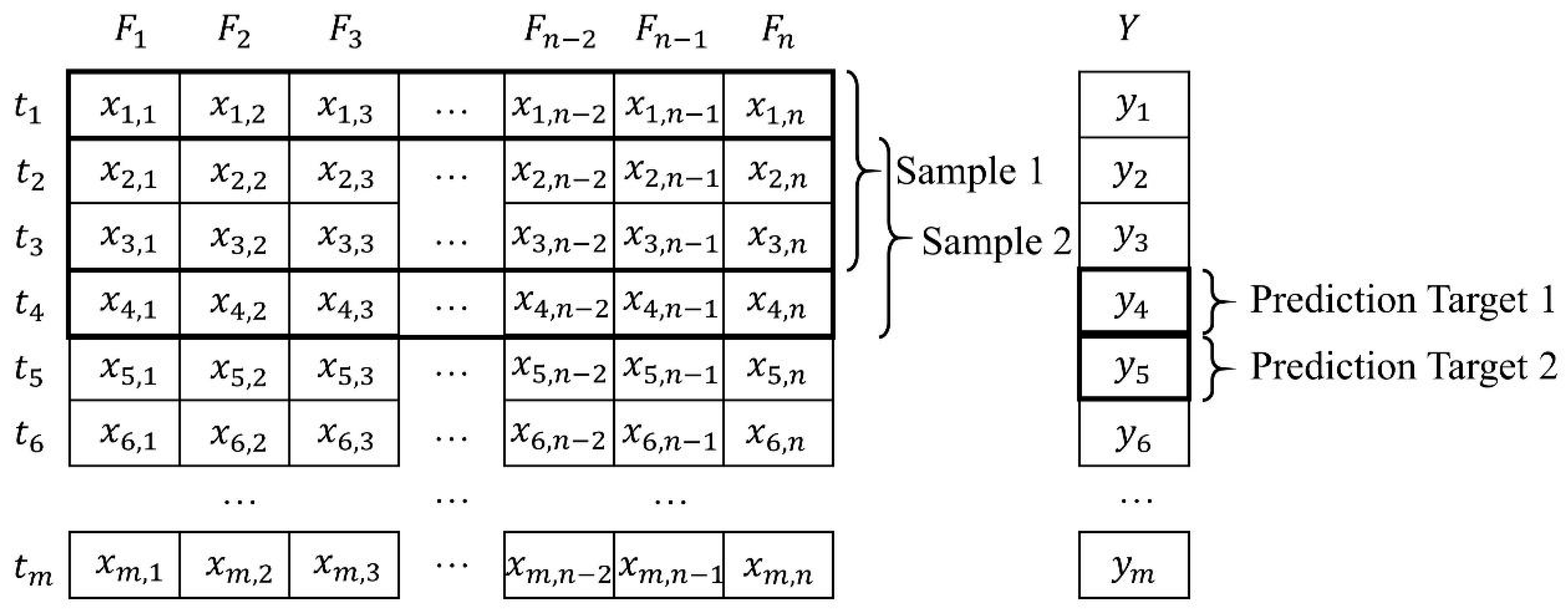
2.1.3. Sliding Window Sampling

A raw input dataset with M rows and N + 1 columns means that it has M records; each has N different features and a prediction target. For the GRU network, since the input should be a sequence with multiple time steps, a sliding window method has been utilized to generate samples. Take the time step (sliding window size) = 3 as an example. The data structure, in addition to the sampling process, is shown in Figure 1. For the input dataset that without a PCA denoising operation, the column index F n represents the hydrological stations or the meteorological stations. For the one with a PCA denoising operation, the column index F n represents a feature. The row index t n means time, which has a unit of day in this research. The Y is the column of the prediction target values.

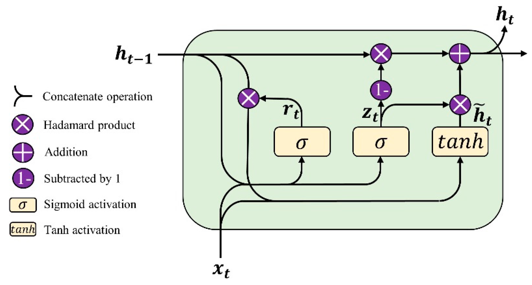
2.2. Gated Recurrent Unit (GRU)

The GRU cell [44] contains two gate units (three gates in some of the literature [59], which include the output gate): the update gate and the reset gate. The internal structure of a primary GRU cell is shown in Figure 2. The unimportant information in the hidden state from the previous time step can be discarded through the reset gate. In contrast, useful information will be retained to affect the current hidden state. The whole forward propagation steps are as shown in Equations (3)–(6):
r t =   σ ( W r · [ h t 1 , x t ] ) ,
z t =   σ ( W z · [ h t 1 , x t ] ) ,
h ˜ t = tan h ( W h ˜ · [ r t h t 1 , x t ] ) ,
h t = ( 1 z t ) h t 1 + z t h ˜ t .
where r t and z t denote the output of the reset gate and the update gate, respectively. σ represents the sigmoid activation function. represents the Hadamard product (element-wise product). [ a , b ] denotes the concatenate operation for two vectors. h t represents the current hidden state.

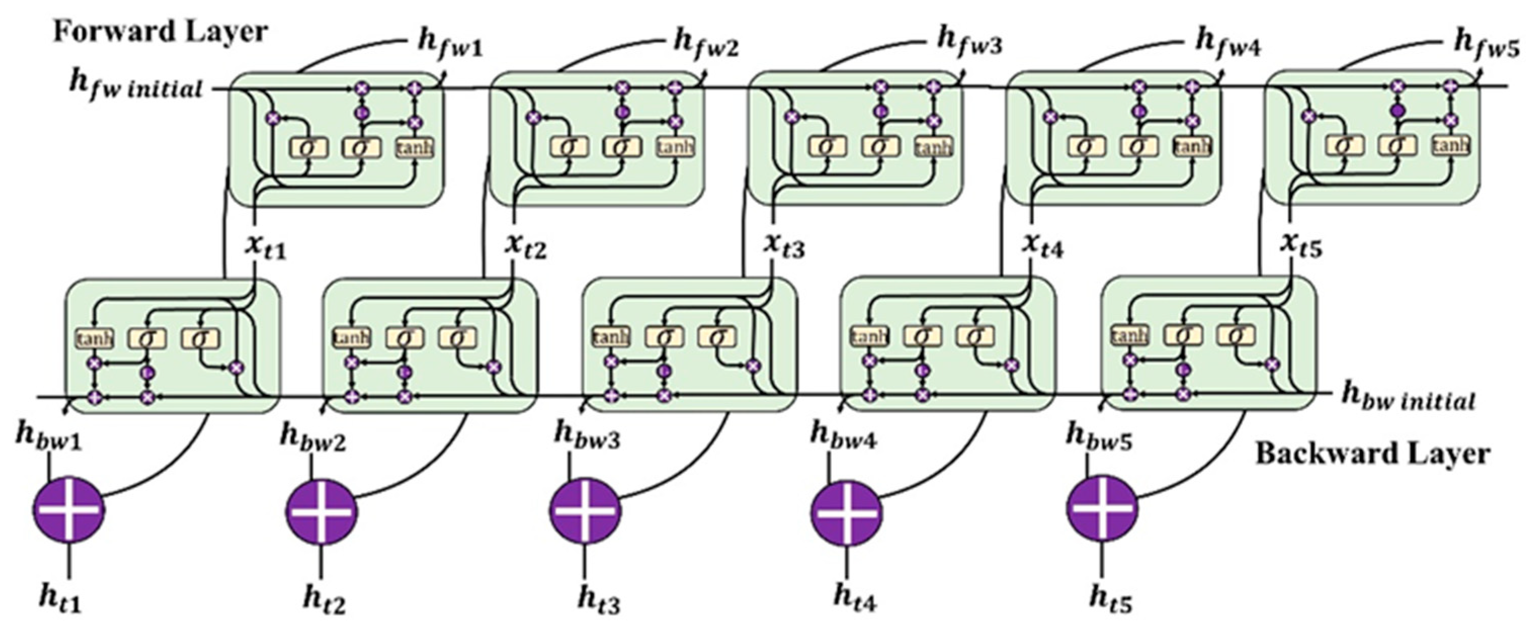
2.3. Stacked and Bi-Directional GRU (bi-GRU)

The combination of several layers of the basic LSTM or GRU cells may enhance the model’s ability when learning the nonlinear relationships and provide a better prediction accuracy [53,60]. The typical structure of a stacked GRU network with two layers is shown in Figure 3. The first layer’s hidden state is utilized as the input of the second layer for further calculations. The result could be obtained from the output of the second layer.
A basic bi-GRU network (Figure 4) has two single layers that propagate in inverse directions. The forward layer uses the first record in the input sequence as the beginning, while the backward layer uses the last record as its beginning. The overall state is the summation of the states from both of the layers; the final state can also be covered by an activation layer.

2.4. Model Evaluation

Nash–Sutcliffe efficiency (NSE), root mean square error (RMSE), and mean absolute error (MAE) has been used in each simulation, as shown in Equations (7)–(9), respectively:
N S E = 1 i = 1 n ( O i P i ) 2 i = 1 n ( O i O ¯ ) 2 ,
R M S E =   1 n i = 1 n ( O i P i ) 2 ,
M A E =   1 n × i = 1 n | O i P i | .
where O i is the observed flowrate, P i is the predicted flowrate, O ¯ is the mean value of the observed flowrate, n is the total number of observations. The NSE values range from to 1. A higher NSE value indicates a better fitting result. Both the RMSE and MAE ranges from 0 to + (with a unit of m3/s in this study), the lower the RMSE and MAE are, the better the model performs. The RMSE is more sensitive to abnormal values than the MAE.
For the robustness evaluation, the mean standard deviation of the abovementioned metrics along the time steps (one of the hyperparameter, that is, the length of input sequence) will be calculated through Equation (10) metrics as mentioned earlier in each scenario:
σ =   1 n i = 1 n ( x i μ i ) 2 .
where σ is the standard deviation, x i is the i th metric, μ i is the mean value of the metrics. The value of standard deviation is greater than 0, a lower standard deviation indicates that the metrics are more aggregated and more robust to time steps.
For the accuracy evaluation, besides the NSE, RMSE, and MAE used in the overall evaluation, the relative error (as shown in Equation (11)) has been used to evaluate the performance on flood peak forecasts:
δ = | O p e a k P p e a k | O p e a k · 100 % .
where δ is the relative error, O p e a k is the observed peak flow, P p e a k is the predicted value of the observed peak flow. The relative error value ranges from 0 to + , the closer the value is to 0, the better the fitting is.

3. Case Study and Materials

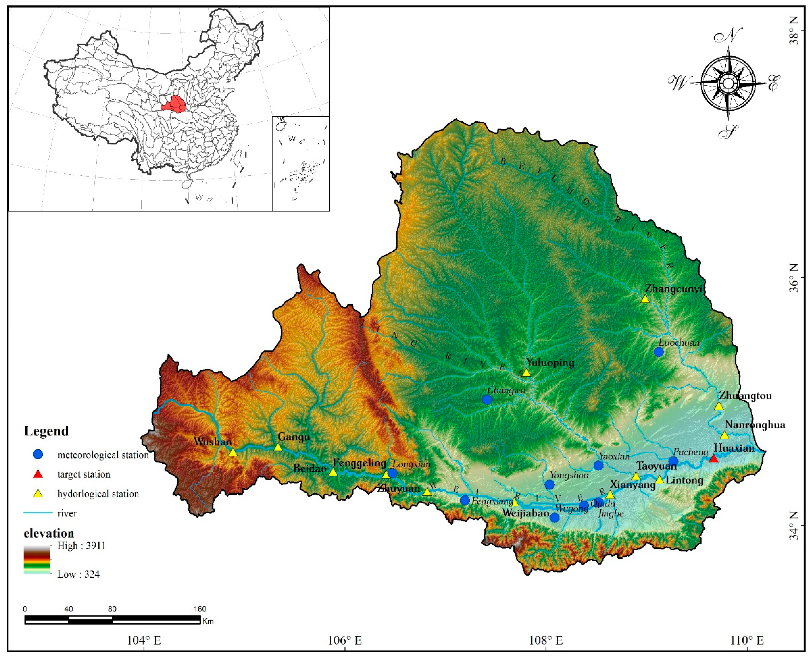
3.1. Research Area and Data

The Wei River basin (33° N~37° N, 104° E~110° E), which is mainly located in Shaanxi Province, China, has an area of 135.9 thousand square kilometers. It is a representative region in the western and northern parts of China. Located in a semi-humid to semi-arid warm temperature climate zone, the basin has a continental monsoon climate [61], and the elevation ranges from 324 m to 3911 m. The downstream region has annual precipitation ranges from 600~800 mm, while the annual precipitation at the upstream region ranges from 350~500 mm. The period from June to October accounts for 65~80% of the total annual precipitation. As a result, the downstream area is affected by flood events frequently. The basin accounts for 64% of the total population, 72% of the irrigation area, and 80% of the GDP in Shaanxi Province from socio-economical activities. Additionally, this basin is located at the Loess Plateau, which is very sensitive to soil erosion caused by rainfall-runoff processes. Hence, stable and reliable runoff forecasting can have high merit for flood warnings, water resources management, and water and soil conservation in this region. The Wei River is the largest tributary of the Huang River containing the main channel and two main branches (the Jing River and the Beiluo River).
The daily runoff data (gotten from the Hydrological Yearbook of the People’s Republic of China) at 14 hydrological stations and the daily rainfall data (gotten from China Meteorological Data Service Center, http://data.cma.cn) at 10 meteorological stations from 2007 to 2014 were collected. Good continuity makes the collected data suitable for the sequential learning model. As a result of the good sufficiency of stations, a vector selection process becomes necessary, the impact of several input combinations can be explored. The research area, the locations of the hydrological and meteorological stations, and the prediction target station are shown in Figure 5. The summaries of the data at the hydrological stations and the meteorological stations are given in Table 1 and Table 2, respectively. The grey relation grade [62] and the Pearson correlation coefficient between each station and the prediction target, Huaxian station, have been calculated to show the data’s relevance.

3.2. Scenarios and Traning Process

As shown in Table 3, six scenarios for both the one-day-ahead and two-day-ahead forecasting have been set to evaluate the impact of different input filtering and model construction strategies. Referring to Figure 5 and Table 1 in Section 3.1, though the Beiluo River is a tributary flowing downstream of the prediction target, the distance from each of the hydrological stations in the Beiluo River basin is relatively close (23.5 km from Nanronghua station, 49.4 km from Zhuangtou station, 158.5 km from Zhangcunyi station). The grey relation analysis and the Pearson correlation analysis show that the data in the Beiluo river basin is also moderately or highly relevant (R = 0.763, 0.757, and 0.409; grey relation grades over 0.99) to the data at the prediction target. Thus, the runoff data from the Beiluo River may be valuable as a reference and should be cautiously evaluated.
Five different input filtering strategies are given from S1 to S5. For the scenarios without PCA denoising operation (from S1 to S4), different rainfall and runoff data combinations have been designed. Evaluating the impact of the inclusion of rainfall data, since the R values and the grey relation grades of the data at meteorological stations are very close (0.094~0.124 and 0.979~0.980, respectively), all the rainfall data from meteorological stations are included in S1 and S3, while excluded in S2 and S4. Also, considering the application of data at similar adjacent regions when using the hydrological analogy method for runoff calculation, to explore whether the similarity would also be valuable to the GRU forecasting model, the runoff data at the stations in the Beiluo River is included in S1 and S2, while excluded in S3 and S4. For the scenarios with PCA denoising operation, S5 and S6 can evaluate the impact of the PCA processed data on the models’ performance.
Furthermore, S6 is given to compare with S5 to illustrate the architecture’s potential influence when constructing the model. The primary GRU cells have been utilized in S5 and the bi-GRU cells in S6.
Forty-eight different combinations of the hyperparameters have been set for each scenario to evaluate the models’ robustness in the model construction process. A summary of the combinations is given in Table 4.
The input dataset (from 2007 to 2014) has been divided into the training set, validation set, and testing set according to a ratio of 6:2:2. The validation dataset has been utilized for all of the hyperparameter combinations in accordance with assessing the impact of different inputs and architectures on the model’s robustness. For accuracy evaluation, both the performance in the validation set and testing have been considered. Additionally, the training dataset has a small batch size of 10 samples. Five hundred epochs have been executed in the training process.

3.3. PCA Denoised Data

The scree plot of the components for the PCA denoising operation is given in Figure 6. According to the scree plot, the explained variance declines dramatically, while the accumulative explained variance increases significantly before the fourth component. Quantitatively, the first four main components explained 91.11% of the variance. This result indicates that the remaining 20 components have contributed limited information (8.89%). Hence, after the PCA denoising operation, four of 24 components are maintained and utilized as the input dataset in scenario S5 and S6 (refer to Table 3 in Section 3.2). It is of note that since the PCA denoising operation is a subjective process, the amount of remaining information could still be optimized (if needed) according to the further training and validation process in the modelling stages.

4. Results and Discussions

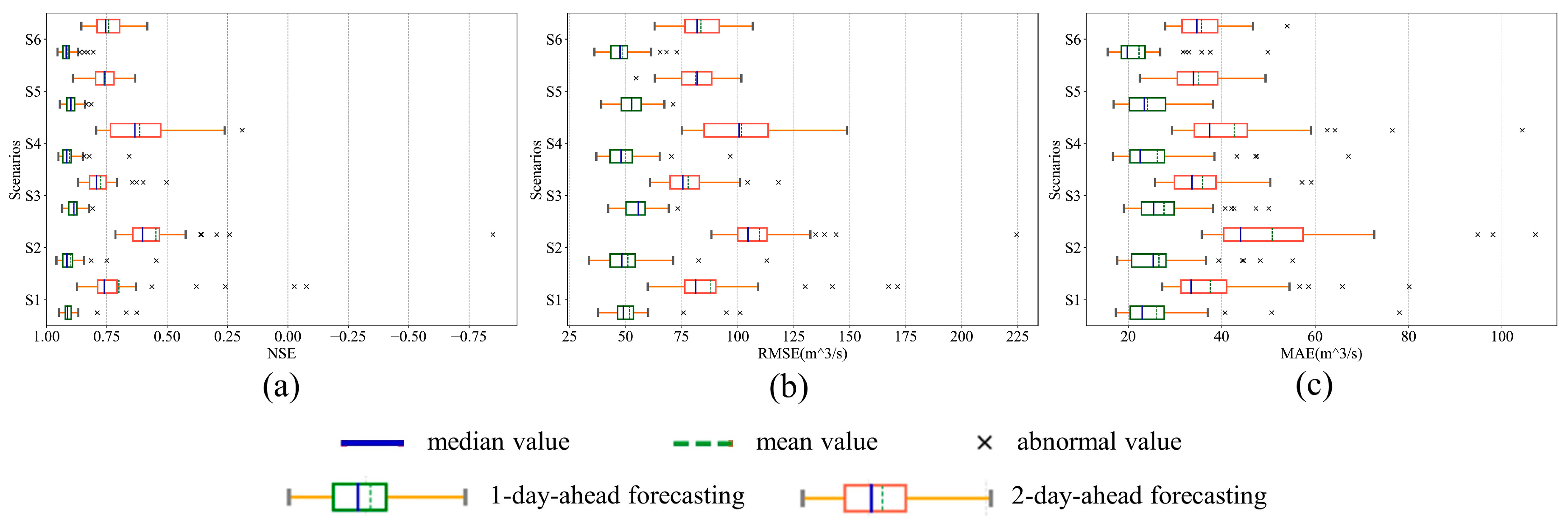
4.1. Robustness Evaluation

4.1.1. Overall Evaluation

Using the validation set to evaluate the model’s robustness to the various hyperparameters, Figure 7a–c show the distribution of NSE, RMSE, and MAE, respectively.
Comparing S1 and S3 with S2 and S4, a lower inter-quartile range (IQR) has been observed in either the distributions of NSE, RMSE, and MAE in both the one-day-ahead (T + 1) and two-day-ahead (T + 2) forecasting. Moreover, this phenomenon is more evident in T + 2 forecasting. This result means that the metrics in S1 and S3 are more aggregated than in S2 and S4. Considering the abnormal values, S1 and S3 also tend to have a higher NSE, a lower RMSE, and a lower MAE than S2 and S4 when bad fitting occurs. Additionally, S1 and S3 also have a higher mean value and median value of NSE, lower ones of RMSE, and lower ones of MAE. These results mean that the model with the rainfall data is less sensitive and of greater robustness to the various hyperparameters and will require less effort on the hyperparameter optimization.
Comparing S1 and S2 with S3 and S4, though significant difference has not been observed from the aspect of IQR for either of the distributions of metrics in both the T + 1 and T + 2 forecasting, the abnormal values indicate that that the inclusion of the runoff data in the adjacent region results in larger deviations when the hyperparameter varies. Thus, though with high numerical relevance, the runoff data in the adjacent region introduces noises and increases the difficulty of the hyperparameter optimization process. Since it is less likely to cause serious deviation, excluding these runoff data can make the model more robust to the hyperparameters.
The metrics’ distribution patterns in S5 and S6 in both the T + 1 and T + 2 forecasting show that the metrics are at least as aggregated as the one in the scenario with the best manual filtered input (S3), indicating that the PCA denoising is an effective input filtering strategy. The PCA denoising operation has significantly improved the model’s robustness to the various hyperparameters with a premise of good forecasting performance. Overall, comparing S6 with S5, the bi-directional architecture does not suggest a significant effect on the robustness of the model to various hyperparameters.

4.1.2. Time Step Standard Deviation of the Evaluation Metrics

As the length of the time step is the most vital hyperparameter that determines the amount of information in the input, the model’s robustness to it should be evaluated independently. Table 5 shows the mean values of the evaluation metrics’ standard deviation when the input time step varies. The higher the values are, the less likely the model to have a stable performance on the metrics. Thus, the model will require more effort in time step optimization. In other words, it will be less robust to the length of the input time steps. Similar to patterns obtained from overall evaluation, from the comparison between S1 and S2, as well as S3 and S4 in either T + 1 or T + 2 forecasting, the inclusion of rainfall data tends to enhance the time step robustness of the model. Additionally, the enhancement effect has been observed to be more evident in T + 2 forecasting. The comparison between S1 and S3 with S2 and S4, correspondingly, shows that though numerically relevant to the prediction target, the runoff data from the adjacent sub-basin will introduce noise and then hinder the model’s time step robustness in the validation stage. Consequently, the time step optimization will be trickier. In comparing S5 and S6, the single directional architecture is more robust than the bi-directional architecture to the time step variations. This phenomenon is different from the overall view and can be explained by the fact that bi-directional architecture is more dependent on the information in the context. When the length of the sequence changes, the amount of information in the context varies.

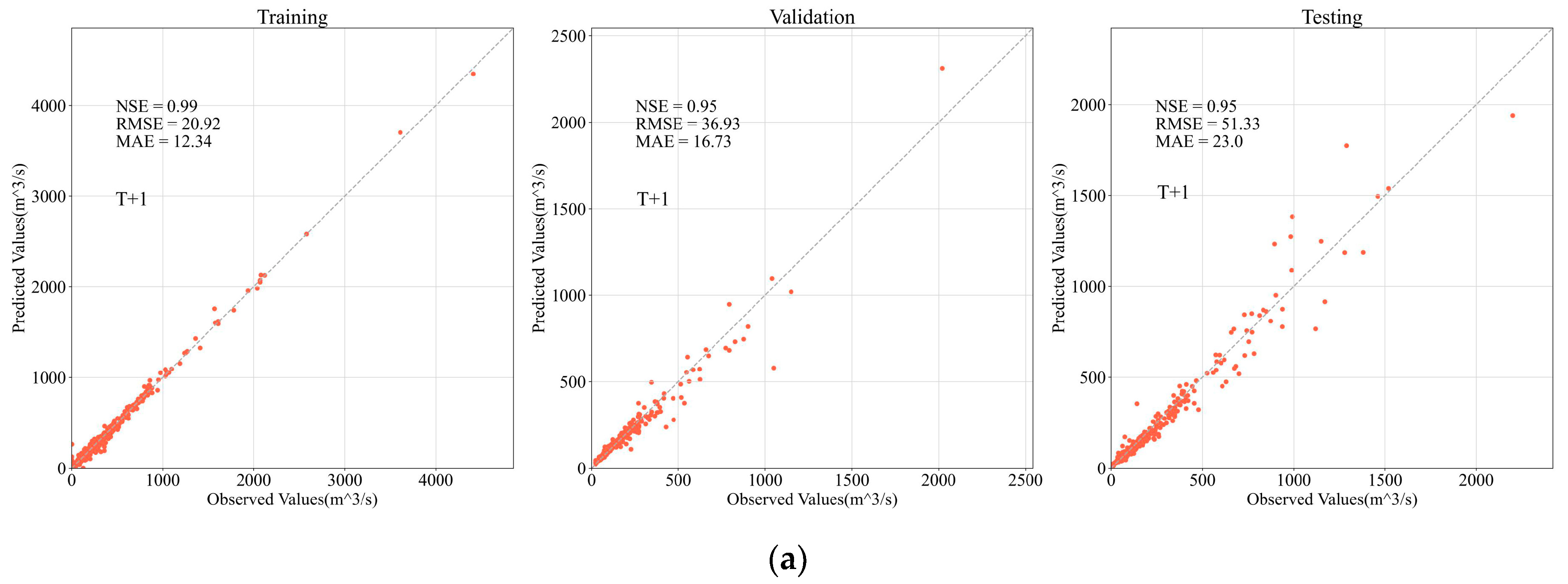
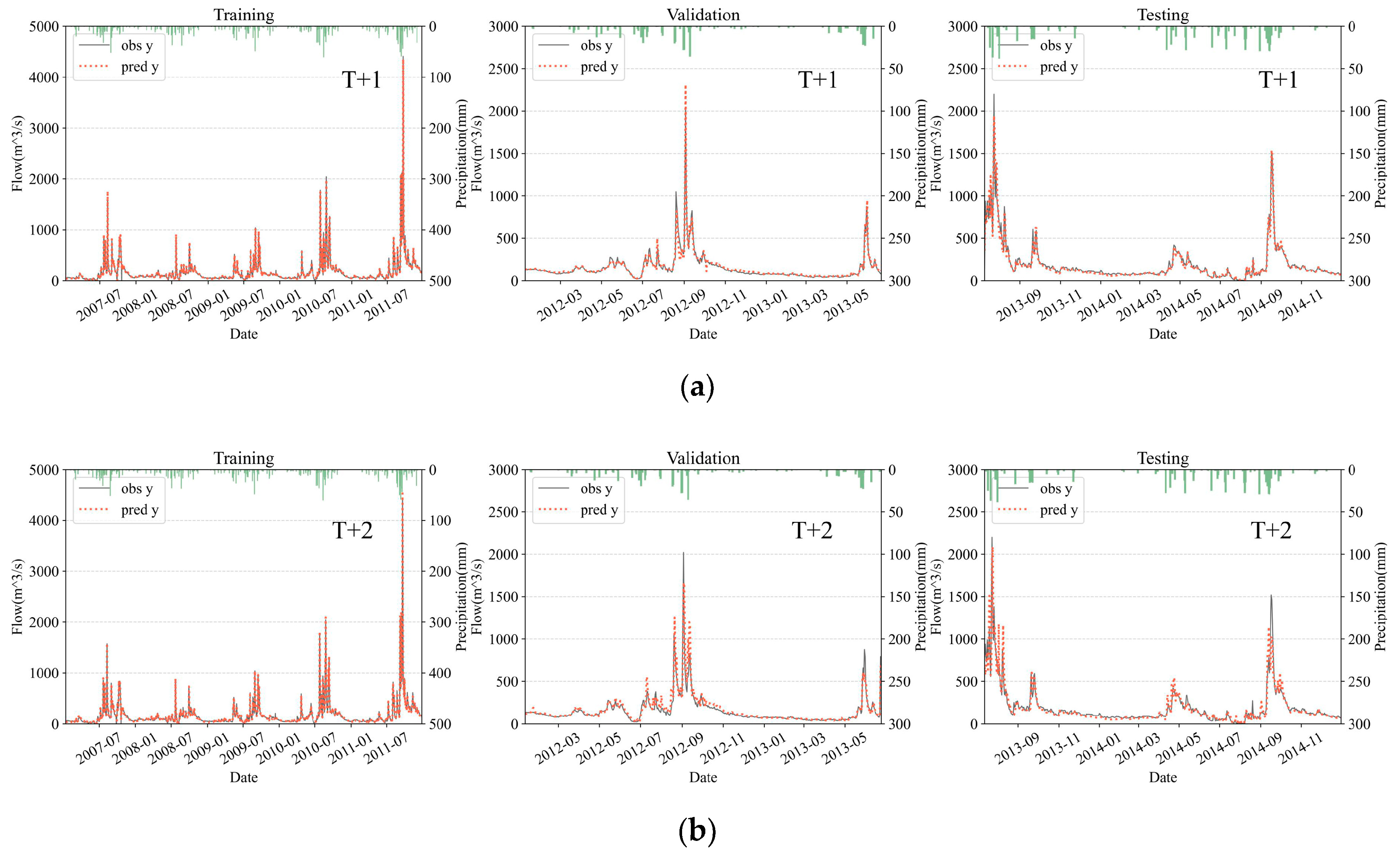
4.2. Accuracy Evaluation

4.2.1. Overall Evaluation

Figure 8 and Figure 9 is the scatter graph and the hydrograph of the best model considering the overall performance in the validation set and testing set for one-day-ahead forecasting and two-day-ahead forecasting. The NSE values in the validation set and the testing set all exceed 0.95, indicating that the model can provide runoff prediction with high precision. The results also suggest that though the forecasting accuracy declines significantly with the increasing lead time, the NSE values are still over 0.83, acceptable, and meaningful for practical use. Furthermore, the scatter plots and the hydrographs show that the apparent deviations are more likely to occur as the flowrate increases. This pattern is more evident in the T + 2 forecasting, in other words, in the forecasting with a longer lead time. From the aspect of the hydrological mechanism, the large flowrates in this research area are usually caused by intensive rainfall processes, in which the infiltration excess (Horton) runoff’s occupancy increases [63]. Since the Horton runoff process driven by intensive rainfalls has a relatively short duration [64], although the runoff data at the distant stations can partially explain the flowrate at the prediction target, it is still difficult for the models to accurately predict the large flowrate two days later. The performance comparison between T + 1 and T + 2 forecastings also shows that the rainfall and runoff data one day before the prediction date is valuable. This can be explained by the fact that in some rainfall-runoff events, the data’s time lags caused by the distance between the prediction target and some adjacent upstream stations are less than two days. Additionally, the deviations when dealing with large flowrates may also be caused by a fact that the weighting matrix does not take the seasonal variation of the rainfall-runoff mechanism [65] into account.
Table 6 shows the overall evaluation metrics (equivalently considered the results of the validation and testing stage) of the best models in different scenarios; the best model for T + 1 forecasting occurs in S4, that is, the scenario without the runoff data in the Beiluo River basin and the rainfall data. In this case, the NSE reaches 0.951, and the RMSE, MAE, has a value of 44.132 m3/s and 19.868 m3/s, respectively. The NSE values in all the scenarios exceed 0.9 for T + 1 forecasting, and in most of the scenarios exceed 0.8 for T + 2 forecasting, which means that either of the input filtering strategies can have an acceptable prediction accuracy after the optimization of hyperparameters. However, there are still some differences determining which kind of strategy is better.
For T + 1 forecasting, comparing S1 with S2, as well as S3 with S4, the NSE in S1 and S3 is correspondingly lower than in S2 and S4. Meanwhile, the RMSE and MAE in S1 and S3 are higher than in S2 and S4. This phenomenon indicates that the inclusion of rainfall data decreases the optimized accuracy when forecasting. The reason is that the rainfall data at some distant stations (e.g., Longxian, 296.9 Km to the prediction target) don’t explain the runoff at the prediction target 1 day later, but are included in S1 and S3 during the training processes. The impact of the inclusion or exclusion of the runoff data in the Beiluo River basin on the optimized forecasting accuracy is not significant through the comparison between S1 and S3, as well as S2 and S4. The results of S5 and S6 that are two scenarios with PCA denoising show that the models with PCA denoised dataset can provide almost the same level of accuracy (NSE reaches 0.945 and 0.946 in S5 and S6) when comparing the best result of the model (has an NSE of 0.951) with manual filtered dataset. The comparison between S5 and S6 indicates that a bi-directional architecture enhanced the overall prediction accuracy.
For T + 2 forecasting, the comparisons between S1 and S2, as well as S3 and S4 (NSE of 0.835 and 0.745 for S1 and S2, 0.836 and 0.801 for S3 and S4) indicating a result that the incorporation of the rainfall data has improved the accuracy of the forecasting results. This result is opposite to the one obtained in one-day-ahead forecasting. It suggests that the rainfall data acts as a noise for the optimized prediction accuracy in one-day-ahead forecasting. However, it is valuable information for the forecasts that have a more extended lead time. This phenomenon can be partly explained by the lag effect in the rainfall-runoff mechanism. Referring to the distances from the meteorological stations to the prediction target given in Table 2 (Section 3.1), almost all the meteorological stations located in the upstream places have a distance of over 100 Km (except for the Pucheng station) to the prediction target. Runoff generated in those places needs time to move to the prediction target. As the result, the rainfall data at those meteorological stations two or more days ago mainly contribute to the flowrate at the prediction target at the forecasting date. These contributions have been recorded in the input time series. Different from the condition in one-day-ahead forecasting, the comparisons between S1 and S3, in addition to S2 and S4, have suggested a significant difference affected by the inclusion or exclusion of the runoff data in the Beiluo River basin. Affected by the noise introduced by the runoff data in the Beiluo River basin, the results in S1 and S2 have lower NSE values (0.835 and 0.745) and higher values of the errors comparing with S3 and S4. The causes of that noise are consequences of the similarities of the runoff data due to the geographic homogeneity between the Beiluo River basin and the prediction target. According to the locations of the hydrological stations, as well as the landscape of the research area (Figure 5), the hydrological stations in the Beiluo River basin are close to the prediction target (Nanronghua, Zhuangtou, and Zhangcunyi have a distance of 23.5, 49.4, and 158.5 Km to the prediction target, respectively), and with a similar underlying surface. For T + 2 forecasting, the runoff data at least two days ago near the prediction target would contain little valuable information. S5 and S6 show that the models with PCA denoising can provide accurate forecasting results with NSE values exceeding 0.82 and are comparable to, even better than the best results generated by the models with manual data filtering strategies. The best model occurs in S6, which means that the bi-directional architecture performs better than the single directional architecture for two-day-ahead forecasting after hyperparameter optimisation. The outperformance of the bi-directional architecture has been claimed by many studies [52,53,60,66] in other domains and is still supported by this research when applying to runoff forecasting.

4.2.2. Accuracy of Flood Peak Forecasts

The peak flow is usually of the greatest interest when carrying out runoff forecasting since it is crucial to flooding alarming. To evaluate the prediction accuracy of the models on the peak flow, we analyzed the maximum flowrate of the flood events in the validation set and testing set. Table 7 shows the relative error of the forecasting results for the selected peak flows.
For the T + 1 forecasting, the comparisons between the mean relative errors of three selected peak flows in S1 and S2, S3 and S4, suggest that the inclusion of the rainfall data exacerbates the error for flood peak forecasts. Le et al. [15] applied the LSTM network into runoff forecasting in the Da River basin (in Vietnam) also obtained a similar result when evaluating the model’s performance on flood peak forecasting. Comparing S1 and S3, S2 and S4, the inclusion of the runoff data in the Beiluo River basin led to smaller errors for the peak flow forecasts. This pattern is slightly different from that in the overall accuracy evaluation, indicating that the adjacent runoff data may not have a significant enhancement effect for the whole forecasting process, but is valuable for the peak flow forecasts with a short lead time. Comparing S5 and S6 to other scenarios, the prediction accuracies of the models with PCA denoising for the peak flows are comparable to the models with manual filtering strategies (relative error ranges in 8.99~12.68% comparing with 6.77~15.90%). Comparing S6 to S5, a bi-directional structure tends to enhance the prediction accuracy of the flood peaks.
For the T + 2 forecasting, contrary to the situation in the T +1 forecasting, rainfall data significantly reduced the relative error of the flood peak forecasts (the mean relative error of the flood peaks in S1 and S3 is 31.41% and 25.37%, while in S2 and S4 is 47.66% and 25.93%). This effect is slightly different from one of the results of the abovementioned relevant study [15] in the Da River basin, Vietnam. The difference is mainly caused by the characteristics of the research areas and flood events. The Da River basin is much smaller than the Wei River basin (52,900 Km2 compared with 135,900 Km2), the time lag effect caused by the distance would not as evident as that in the Wei River basin. The rainfall in that basin is also more intensive. Additionally, the flood event evaluated in that study has a peak flow of over 10,000 m3/s, indicating a much shorter duration compared with the one in this study. Thus, the rainfall data in the Da River basin does not explain the flood event well. Hence, significant differences in the characteristic of the research area would partially make the patterns vary. The mean error of the flood peaks in S1 and S2 is correspondingly higher than in S3 and S4, revealing that the inclusion of the runoff data from the Beiluo River basin significantly increased the prediction deviation. These phenomena show that, though the rainfall data acts as a noise for T + 1 forecasts, it can explain the runoff two days later; some information contained in the runoff data in the adjacent region is valuable for the T + 1 forecasts since the similarity to the data at the prediction target but acts as a noise for the T + 2 forecasts. The comparison between S5, S6, and other scenarios, suggesting that the models with PCA denoising can have a better performance on the peak flow forecasts when the lead time increases. The PCA has effectively filtered the noise and remained valuable information. Similar to that in the T + 1 forecasting, the bi-directional architecture has enhanced the peak flow forecasts’ accuracy.

4.3. Recommendations Based on the Evaluation Results

Some recommendations for future studies and applications of the GRU runoff forecasting model can be provided according to the evaluation results. Considering both the robustness evaluation and accuracy, for the models with manual vector selection preprocessing process, the rainfall data is recommended to be included as the input, especially in long-lead-time forecasts. To be mentioned, this recommendation is mainly based on a premise that the rainfall data is sufficient, however, as the acquisition of rainfall data is difficult in some study areas, the continuous hydrologic modelling [67,68,69] for design simulation would be a potential supplement. In short-lead-time flood forecasts, it can be considered to be excluded since a negative impact on the optimized prediction accuracy. The runoff data from some adjacent tributaries may be valuable for short-lead-time forecasts for the main channel but is strongly suggested to be excluded when the lead time increases. The PCA denoised dataset can make the model more robust and with equivalent accuracy comparing with the manually filtered dataset, thus, we recommend using the PCA as an alternative preprocessing method. The advantage of the PCA when applying to the preprocessing stage in machine learning is also supported by studies in other realms [56,58,70,71]. Similar to the results of the research about NLP [36,72] and other topics [53,73,74], the bi-directional RNN architecture also tends to provide more accurate results and is recommended to be utilized in the GRU runoff forecasting model.
For further studies, more data filtering strategies can be tested. For instance, the runoff data close to the river’s source or the runoff data at the upstream tributaries has a low correlation coefficient. The impact of the inclusion or exclusion of this data will also be valuable for other researchers. The seasonal variation can be considered as an attempt to improve the performance of the model. Furthermore, the type of research area will also affect the found patterns and can be explored in the future.

5. Conclusions

This research studied the impact of different input filtering strategies and the model construction strategies on the robustness and prediction accuracy of the GRU model. For the input filtering strategies, the impact of the rainfall data, runoff data at the adjacent region with medium to the high correlation coefficient, and PCA denoising operation has been assessed. For the model construction strategies, we have tested single directional architecture and bi-directional architecture. In summary, the main findings of this study include:
  • Based on the premise that the rainfall data is sufficient, its inclusion can enhance the model’s robustness when the hyperparameters vary. Additionally, when the lead time increases, this enhancement effect becomes more pronounced. For optimized accuracy, the rainfall data has a negative impact on the forecasts with a short lead time but is valuable for the forecasts with a longer one in either the overall forecasting process or the flood peak forecasting process. Therefore, the rainfall data is recommended to be included in long-lead-time forecasts.
  • Though a relative high relevance to the prediction target, the runoff data at the adjacent tributary introduces noise that significantly hinders the robustness of the model and will increase the difficulty of the optimization of hyperparameters. Nevertheless, this runoff data also contains valuable information for the flood peak forecasts with a short lead time and, thus, the exclusion of it should be carefully considered according to the purpose of use. For the forecasts with a more extended lead time, this data acts as noise and should be excluded.
  • The model uses PCA denoising as the input filtering strategy has comparable robustness to the model that uses well manually filtered data as the input. Thus, it can reduce much effort in the data filtering stage. Meanwhile, the model with PCA denoising operation can provide accurate forecasts, especially for the flood peak forecasts when the lead time increases. Thus, the PCA denoising can be an efficient substitution for the manual input filtering process and is recommended to be considered as an alternative preprocessing method in the future.
  • Despite a slightly lower time-step robustness, the bi-directional architecture has higher prediction accuracy than the single directional architecture for runoff forecasting, therefore, it is suggested to be utilized.
Though the amount of considered input filtering strategies, as well as the combinations of hyperparameters, in addition to the considered architectures, are still limited, the research has revealed some meaningful patterns in defined conditions. It could be a reference for other researchers in the data filtering and model construction stages.

Author Contributions

Conceptualization: Q.W.; methodology: Q.Y.; software: Q.W.; formal analysis: Q.W., Y.L.; resources: X.Y.; data curation: X.Y.; writing—original draft preparation: Q.W.; writing—review and editing: Y.L.; visualization: Y.Z.; supervision: J.Y.; project administration: J.Y.; funding acquisition: J.Y. All authors have read and agreed to the published version of the manuscript.

Funding

This research was funded by the National Natural Science Foundation of China, grant number 51779007, and the National Key Research and Development Program of China, grant number 2016YFC0401308.

Conflicts of Interest

The authors declare no conflict of interest.

References

  1. Narbondo, S.; Gorgoglione, A.; Crisci, M.; Chreties, C. Enhancing Physical Similarity Approach to Predict Runoff in Ungauged Watersheds in Sub-Tropical Regions. Water 2020, 12, 528. [Google Scholar] [CrossRef] [Green Version]
  2. Navas, R.; Alonso, J.; Gorgoglione, A.; Vervoort, R.W. Identifying Climate and Human Impact Trends in Streamflow: A Case Study in Uruguay. Water 2019, 11, 1433. [Google Scholar] [CrossRef] [Green Version]
  3. Nazari-Sharabian, M.; Taheriyoun, M.; Ahmad, S.; Karakouzian, M.; Ahmadi, A. Water Quality Modeling of Mahabad Dam Watershed–Reservoir System under Climate Change Conditions, Using SWAT and System Dynamics. Water 2019, 11, 394. [Google Scholar] [CrossRef] [Green Version]
  4. Kratzert, F.; Klotz, D.; Herrnegger, M.; Sampson, A.K.; Hochreiter, S.; Nearing, G.S. Toward Improved Predictions in Ungauged Basins: Exploiting the Power of Machine Learning. Water Resour. Res. 2019, 55, 11344–11354. [Google Scholar] [CrossRef] [Green Version]
  5. Ahmed, U.; Mumtaz, R.; Anwar, H.; Shah, A.A.; Irfan, R. Efficient Water Quality Prediction Using Supervised Machine Learning. Water 2019, 11, 2210. [Google Scholar] [CrossRef] [Green Version]
  6. Liang, J.; Li, W.; Bradford, S.A.; Šimůnek, J. Physics-Informed Data-Driven Models to Predict Surface Runoff Water Quantity and Quality in Agricultural Fields. Water 2019, 11, 200. [Google Scholar] [CrossRef] [Green Version]
  7. Busico, G.; Colombani, N.; Fronzi, D.; Pellegrini, M.; Tazioli, A.; Mastrocicco, M. Evaluating SWAT model performance, considering different soils data input, to quantify actual and future runoff susceptibility in a highly urbanized basin. J. Environ. Manag. 2020, 266, 110625. [Google Scholar] [CrossRef]
  8. Duan, Y.; Meng, F.; Liu, T.; Huang, Y.; Luo, M.; Xing, W.; De Maeyer, P. Sub-Daily Simulation of Mountain Flood Processes Based on the Modified Soil Water Assessment Tool (SWAT) Model. Int. J. Environ. Res. Public Health 2019, 16, 3118. [Google Scholar] [CrossRef] [Green Version]
  9. Fereidoon, M.; Koch, M.; Brocca, L. Predicting Rainfall and Runoff Through Satellite Soil Moisture Data and SWAT Modelling for a Poorly Gauged Basin in Iran. Water 2019, 11, 594. [Google Scholar] [CrossRef] [Green Version]
  10. Wang, G.; Zhou, M.; Takeuchi, K.; Ishidaira, H. Improved version of BTOPMC model and its application in event-based hydrologic simulations. J. Geogr. Sci. 2007, 17, 73–84. [Google Scholar] [CrossRef]
  11. Peng, Y.; Sun, X.; Zhang, X.; Zhou, H.; Zhang, Z. A Flood Forecasting Model that Considers the Impact of Hydraulic Projects by the Simulations of the Aggregate reservoir’s Retaining and Discharging. Water Resour. Manag. 2017, 31, 1031–1045. [Google Scholar] [CrossRef]
  12. Paparrizos, S.; Maris, F. Hydrological simulation of Sperchios River basin in Central Greece using the MIKE SHE model and geographic information systems. Appl. Water Sci. 2017, 7, 591–599. [Google Scholar] [CrossRef] [Green Version]
  13. Xevi, E.; Christiaens, K.; Espino, A.; Sewnandan, W.; Mallants, D.; Sørensen, H.; Feyen, J. Calibration, Validation and Sensitivity Analysis of the MIKE-SHE Model Using the Neuenkirchen Catchment as Case Study. Water Resour. Manag. 1997, 11, 219–242. [Google Scholar] [CrossRef]
  14. Tan, M.L.; Ramli, H.P.; Tam, T.H. Effect of DEM Resolution, Source, Resampling Technique and Area Threshold on SWAT Outputs. Water Resour. Manag. 2018, 32, 4591–4606. [Google Scholar] [CrossRef]
  15. Le, X.H.; Ho, H.V.; Lee, G.; Jung, S. Application of Long Short-Term Memory (LSTM) Neural Network for Flood Forecasting. Water 2019, 11, 1387. [Google Scholar] [CrossRef] [Green Version]
  16. Tikhamarine, Y.; Souag-Gamane, D.; Ahmed, A.N.; Sammen, S.S.; Kisi, O.; Huang, Y.F.; El-Shafie, A. Rainfall-runoff modelling using improved machine learning methods: Harris hawks optimizer vs. particle swarm optimization. J. Hydrol. 2020, 589, 125133. [Google Scholar] [CrossRef]
  17. Parisouj, P.; Mohebzadeh, H.; Lee, T. Employing Machine Learning Algorithms for Streamflow Prediction: A Case Study of Four River Basins with Different Climatic Zones in the United States. Water Resour. Manag. 2020, 34, 4113–4131. [Google Scholar] [CrossRef]
  18. Thapa, S.; Zhao, Z.; Li, B.; Lu, L.; Fu, D.; Shi, X.; Tang, B.; Qi, H. Snowmelt-Driven Streamflow Prediction Using Machine Learning Techniques (LSTM, NARX, GPR, and SVR). Water 2020, 12, 1743. [Google Scholar] [CrossRef]
  19. Ghorbani, M.A.; Deo, R.C.; Kim, S.; Hasanpour Kashani, M.; Karimi, V.; Izadkhah, M. Development and evaluation of the cascade correlation neural network and the random forest models for river stage and river flow prediction in Australia. Soft Comput. 2020, 24, 12079–12090. [Google Scholar] [CrossRef]
  20. Orellana-Alvear, J.; Celleri, R.; Rollenbeck, R.; Muñoz, P.; Contreras, P.; Bendix, J. Assessment of Native Radar Reflectivity and Radar Rainfall Estimates for Discharge Forecasting in Mountain Catchments with a Random Forest Model. Remote Sens. 2020, 12, 1986. [Google Scholar] [CrossRef]
  21. Song, T.; Ding, W.; Wu, J.; Liu, H.; Zhou, H.; Chu, J. Flash Flood Forecasting Based on Long Short-Term Memory Networks. Water 2020, 12, 109. [Google Scholar] [CrossRef] [Green Version]
  22. Poonia, V.; Tiwari, H.L. Rainfall-runoff modeling for the Hoshangabad Basin of Narmada River using artificial neural network. Arab. J. Geosci. 2020, 13, 1–10. [Google Scholar] [CrossRef]
  23. Ali, S.; Shahbaz, M. Streamflow forecasting by modeling the rainfall–streamflow relationship using artificial neural networks. Model. Earth Syst. Environ. 2020, 6, 1645–1656. [Google Scholar] [CrossRef]
  24. Wagena, M.B.; Goering, D.; Collick, A.S.; Bock, E.; Fuka, D.R.; Buda, A.; Easton, Z.M. Comparison of short-term streamflow forecasting using stochastic time series, neural networks, process-based, and Bayesian models. Environ. Model. Softw. 2020, 126, 104669. [Google Scholar] [CrossRef]
  25. Unnikrishnan, P.; Jothiprakash, V. Hybrid SSA-ARIMA-ANN Model for Forecasting Daily Rainfall. Water Resour. Manag. 2020, 34, 3609–3623. [Google Scholar] [CrossRef]
  26. Saha, A.; Singh, K.N.; Ray, M.; Rathod, S. A hybrid spatio-temporal modelling: An application to space-time rainfall forecasting. Theor. Appl. Climatol. 2020, 1–12. [Google Scholar] [CrossRef]
  27. Ghamariadyan, M.; Imteaz, M.A. A wavelet artificial neural network method for medium-term rainfall prediction in Queensland (Australia) and the comparisons with conventional methods. Int. J. Climatol. 2020, 2020, 1–21. [Google Scholar] [CrossRef]
  28. Tikhamarine, Y.; Malik, A.; Souag-Gamane, D.; Kisi, O. Artificial intelligence models versus empirical equations for modeling monthly reference evapotranspiration. Environ. Sci. Pollut. Res. 2020, 27, 30001–30019. [Google Scholar] [CrossRef]
  29. Ferreira, L.B.; Da Cunha, F.F. New approach to estimate daily reference evapotranspiration based on hourly temperature and relative humidity using machine learning and deep learning. Agric. Water Manag. 2020, 234, 106113. [Google Scholar] [CrossRef]
  30. Kao, I.F.; Zhou, Y.; Chang, L.C.; Chang, F.J. Exploring a Long Short-Term Memory based Encoder-Decoder framework for multi-step-ahead flood forecasting. J. Hydrol. 2020, 583, 124631. [Google Scholar] [CrossRef]
  31. Han, Z.; Dian, Y.; Xia, H.; Zhou, J.; Jian, Y.; Yao, C.; Wang, X.; Li, Y. Comparing Fully Deep Convolutional Neural Networks for Land Cover Classification with High-Spatial-Resolution Gaofen-2 Images. ISPRS Int. J. Geo-Inf. 2020, 9, 478. [Google Scholar] [CrossRef]
  32. Collazos-Huertas, D.F.; Alvarez-Meza, A.M.; Acosta-Medina, C.D.; Castaño-Duque, G.A.; Castellanos-Dominguez, G. CNN-based framework using spatial dropping for enhanced interpretation of neural activity in motor imagery classification. Brain Inform. 2020, 7, 1–13. [Google Scholar] [CrossRef] [PubMed]
  33. Hu, F.; Xia, G.; Member, S. Mining Deep Semantic Representations for Scene Classification of High-Resolution Remote Sensing Imagery. IEEE Trans. Big Data. 2020, 6, 522–536. [Google Scholar] [CrossRef]
  34. Sabour, S.; Frosst, N.; Hinton, G.E. Dynamic routing between capsules. Adv. Neural Inf. Process. Syst. 2017, 30, 3857–3867. [Google Scholar]
  35. Hochreiter, S.; Schmidhuber, J. Long Short-Term Memory. Neural Comput. 1997, 9, 1735–1780. [Google Scholar] [CrossRef]
  36. Jang, B.; Kim, M.; Harerimana, G.; Kang, S.U.; Kim, J.W. Bi-LSTM Model to Increase Accuracy in Text Classification: Combining Word2vec CNN and Attention Mechanism. Appl. Sci. 2020, 10, 5841. [Google Scholar] [CrossRef]
  37. Zhu, Y.; Gao, X.; Zhang, W.; Liu, S.; Zhang, Y. A Bi-Directional LSTM-CNN Model with Attention for Aspect-Level Text Classification. Future Internet 2018, 10, 116. [Google Scholar] [CrossRef] [Green Version]
  38. Jelodar, H.; Wang, Y.; Orji, R.; Huang, H. Deep Sentiment Classification and Topic Discovery on Novel Coronavirus or COVID-19 Online Discussions: NLP Using LSTM Recurrent Neural Network Approach. IEEE J. Biomed. Health Inform. 2020, 24, 1. [Google Scholar] [CrossRef]
  39. Zou, Q.; Xiong, Q.; Li, Q.; Yi, H.; Yu, Y.; Wu, C. A water quality prediction method based on the multi-time scale bidirectional long short-term memory network. Environ. Sci. Pollut. Res. 2020, 27, 16853–16864. [Google Scholar] [CrossRef]
  40. Liu, D.R.; Lee, S.J.; Huang, Y.; Chiu, C.J. Air pollution forecasting based on attention-based LSTM neural network and ensemble learning. Expert Syst. 2020, 37, 1–16. [Google Scholar] [CrossRef]
  41. Song, C.; Zhang, H. Study on turbidity prediction method of reservoirs based on long short term memory neural network. Ecol. Model. 2020, 432, 109210. [Google Scholar] [CrossRef]
  42. Wang, C.; Qi, Y.; Zhu, G. Deep learning for predicting the occurrence of cardiopulmonary diseases in Nanjing, China. Chemosphere 2020, 257, 127176. [Google Scholar] [CrossRef] [PubMed]
  43. Goluguri, N.V.R.R.; Devi, K.S.; Srinivasan, P. Rice-net: An efficient artificial fish swarm optimization applied deep convolutional neural network model for identifying the Oryza sativa diseases. Neural Comput. Appl. 2020, 1–16. [Google Scholar] [CrossRef]
  44. Cho, K.; Van Merriënboer, B.; Gulcehre, C.; Bahdanau, D.; Bougares, F.; Schwenk, H.; Bengio, Y. Learning phrase representations using RNN encoder-decoder for statistical machine translation. In Proceedings of the Conference on Empirical Methods in Natural Language Processing (EMNLP 2014), Doha, Qatar, 25–29 October 2014; pp. 1724–1734. [Google Scholar] [CrossRef]
  45. Wang, C.; Du, W.; Zhu, Z.; Yue, Z. The real-time big data processing method based on LSTM or GRU for the smart job shop production process. J. Algorithms Comput. Technol. 2020, 14, 1–9. [Google Scholar] [CrossRef]
  46. Gao, S.; Huang, Y.; Zhang, S.; Han, J.; Wang, G.; Zhang, M.; Lin, Q. Short-term runoff prediction with GRU and LSTM networks without requiring time step optimization during sample generation. J. Hydrol. 2020, 589, 125188. [Google Scholar] [CrossRef]
  47. Li, W.; Kiaghadi, A.; Dawson, C. Exploring the best sequence LSTM modeling architecture for flood prediction. Neural Comput. Appl. 2020, 3, 1–10. [Google Scholar] [CrossRef]
  48. Wu, Y.; Ding, Y.; Zhu, Y.; Feng, J.; Wang, S. Complexity to Forecast Flood: Problem Definition and Spatiotemporal Attention LSTM Solution. Complexity 2020, 2020, 1–13. [Google Scholar] [CrossRef]
  49. Chen, X.; Huang, J.; Han, Z.; Gao, H.; Liu, M.; Li, Z.; Liu, X.; Li, Q.; Qi, H.; Huang, Y. The importance of short lag-time in the runoff forecasting model based on long short-term memory. J. Hydrol. 2020, 589, 125359. [Google Scholar] [CrossRef]
  50. Okkan, U.; Kirdemir, U. Towards a hybrid algorithm for the robust calibration of rainfall-runoff models. J. Hydroinform. 2020, 22, 876–899. [Google Scholar] [CrossRef]
  51. Li, W.; Kiaghadi, A.; Dawson, C. High temporal resolution rainfall–runoff modeling using long-short-term-memory (LSTM) networks. Neural Comput. Appl. 2020, 6. [Google Scholar] [CrossRef]
  52. Shahid, F.; Zameer, A.; Muneeb, M. Predictions for COVID-19 with deep learning models of LSTM, GRU and Bi-LSTM. Chaos Solitons Fractals 2020, 140, 110212. [Google Scholar] [CrossRef] [PubMed]
  53. Atef, S.; Eltawil, A.B. Assessment of stacked unidirectional and bidirectional long short-term memory networks for electricity load forecasting. Electr. Power Syst. Res. 2020, 187, 106489. [Google Scholar] [CrossRef]
  54. Yang, T.; Zhang, Q.; Wan, X.; Li, X.; Wang, Y.; Wang, W. Comprehensive ecological risk assessment for semi-arid basin based on conceptual model of risk response and improved TOPSIS model-a case study of Wei River Basin, China. Sci. Total Environ. 2020, 719, 137502. [Google Scholar] [CrossRef] [PubMed]
  55. Tang, S.; Jiang, J.; Zheng, Y.; Hong, Y.; Chung, E.S.; Shamseldin, A.Y.; Wei, Y.; Wang, X. Robustness analysis of storm water quality modelling with LID infrastructures from natural event-based field monitoring. Sci. Total Environ. 2021, 753, 142007. [Google Scholar] [CrossRef] [PubMed]
  56. Geng, D.; Zhang, H.; Wu, H. Short-Term Wind Speed Prediction Based on Principal Component Analysis and LSTM. Appl. Sci. 2020, 10, 4416. [Google Scholar] [CrossRef]
  57. Bhagat, S.K.; Tiyasha, T.; Awadh, S.M.; Tung, T.M.; Jawad, A.H.; Yaseen, Z.M. Prediction of sediment heavy metal at the Australian Bays using newly developed hybrid artificial intelligence models. Environ. Pollut. 2021, 268, 115663. [Google Scholar] [CrossRef]
  58. Arozi, M.; Caesarendra, W.; Ariyanto, M.; Munadi, M.; Setiawan, J.D.; Glowacz, A. Pattern Recognition of Single-Channel sEMG Signal Using PCA and ANN Method to Classify Nine Hand Movements. Symmetry 2020, 12, 541. [Google Scholar] [CrossRef] [Green Version]
  59. Huang, C.J.; Shen, Y.; Chen, Y.H.; Chen, H.C. A novel hybrid deep neural network model for short-term electricity price forecasting. Int. J. Energy Res. 2020, 1–22. [Google Scholar] [CrossRef]
  60. Crisóstomo de Castro Filho, H.; Abílio de Carvalho Júnior, O.; Ferreira de Carvalho, O.L.; Pozzobon de Bem, P.; dos Santos de Moura, R.; Olino de Albuquerque, A.; Rosa Silva, C.; Guimarães Ferreira, P.H.; Fontes Guimarães, R.; Trancoso Gomes, R.A. Rice crop detection using LSTM, Bi-LSTM, and machine learning models from Sentinel-1 time series. Remote Sens. 2020, 12, 2655. [Google Scholar] [CrossRef]
  61. Duan, L.; Wang, W.; Sun, Y.; Zhang, C.; Sun, Y. Hydrogeochemical Characteristics and Health Effects of Iodine in Groundwater in Wei River Basin. Expo. Health 2020, 12, 369–383. [Google Scholar] [CrossRef]
  62. Zeng, G.; Jiang, R.; Huang, G.; Xu, M.; Li, J. Optimization of wastewater treatment alternative selection by hierarchy grey relational analysis. J. Environ. Manag. 2007, 82, 250–259. [Google Scholar] [CrossRef] [PubMed]
  63. Peng, D.; Xu, Z.; Qiu, L.; Zhao, W. Distributed rainfall-runoff simulation for an unclosed river basin with complex river system: A case study of lower reach of the Wei River, China. J. Flood Risk Manag. 2016, 9, 169–177. [Google Scholar] [CrossRef]
  64. Müller, E.N.; van Schaik, L.; Blume, T.; Bronstert, A.; Carus, J.; Fleckenstein, J.H.; Fohrer, N.; Gerke, H.H.; Graeff, T.; Hesse, C.; et al. Herausforderungen der ökohydrologischen Forschung in Deutschland. Hydrol. Wasserbewirtsch. 2014, 58, 221–240. [Google Scholar] [CrossRef]
  65. Deb, P.; Kiem, A.S.; Willgoose, G. Mechanisms influencing non-stationarity in rainfall-runoff relationships in southeast Australia. J. Hydrol. 2019, 571, 749–764. [Google Scholar] [CrossRef]
  66. Chen, X.; He, J.; Wu, X.; Yan, W.; Wei, W. Sleep staging by bidirectional long short-term memory convolution neural network. Futur. Gener. Comput. Syst. 2020, 109, 188–196. [Google Scholar] [CrossRef]
  67. Grimaldi, S.; Nardi, F.; Piscopia, R.; Petroselli, A.; Apollonio, C. Continuous hydrologic modelling for design simulation in small and ungauged basins: A step forward and some tests for its practical use. J. Hydrol. 2020, 125664. [Google Scholar] [CrossRef]
  68. Petroselli, A.; Grimaldi, S. Design hydrograph estimation in small and fully ungauged basins: A preliminary assessment of the EBA4SUB framework. J. Flood Risk Manag. 2018, 11, S197–S210. [Google Scholar] [CrossRef]
  69. Piscopia, R.; Petroselli, A.; Grimaldi, S. A software package for predicting design-flood hydrographs in small and ungauged basins. J. Agric. Eng. 2015, 46, 74–84. [Google Scholar] [CrossRef] [Green Version]
  70. Nguyen, M.D.; Pham, B.T.; Ho, L.S.; Ly, H.B.; Le, T.T.; Qi, C.; Le, V.M.; Le, L.M.; Prakash, I.; Son, L.H.; et al. Soft-computing techniques for prediction of soils consolidation coefficient. Catena 2020, 195, 104802. [Google Scholar] [CrossRef]
  71. Canchala, T.; Alfonso-Morales, W.; Carvajal-Escobar, Y.; Cerón, W.L.; Caicedo-Bravo, E. Monthly rainfall anomalies forecasting for southwestern Colombia using artificial neural networks approaches. Water 2020, 12, 2628. [Google Scholar] [CrossRef]
  72. Premjith, B.; Kumar, M.A.; Soman, K.P. Neural Machine Translation System for English to Indian Language Translation Using MTIL Parallel Corpus. J. Intell. Syst. 2019, 28, 387–398. [Google Scholar] [CrossRef]
  73. Shahmohammadi, H.; Dezfoulian, M.H.; Mansoorizadeh, M. Paraphrase detection using LSTM networks and handcrafted features. Multimed. Tools Appl. 2020, 1–14. [Google Scholar] [CrossRef]
  74. Kwak, G.; Ahn, C.P.H.; Park, K.L.N. Potential of Bidirectional Long Short-Term Memory Networks for Crop Classification with Multitemporal Remote Sensing Images. Korean J. Remote Sens. 2020, 36, 515–525. [Google Scholar]
Figure 1. An example of the sliding window method, F denotes the feature column, and t denotes a record (or sample).
Water 12 03532 g001
Figure 2. The structure of a basic GRU cell.
Water 12 03532 g002
Figure 3. The typical structure of a double layer stacked GRU network, the second layer obtains the state of the first layer for further calculation.
Water 12 03532 g003
Figure 4. The typical structure of a bi-GRU network with two single layers.
Water 12 03532 g004
Figure 5. The research area with the locations of hydrological and meteorological stations, in addition to the prediction target. The whole basin can be divided into three main sub-basins, which are the main channel basin of the Wei River, the Jing River basin, and the Beiluo River basin.
Water 12 03532 g005
Figure 6. Scree plot of the components, the green line represents the accumulative explained variance ratio, the red line represents the explained variance ratio of each component.
Water 12 03532 g006
Figure 7. Box plots of the distribution of evaluation metrics in the validation stage. (a) Box plot of the distribution of NSE; (b) box plot of the distribution of RMSE; (c) box plot of the distribution of MAE.
Water 12 03532 g007
Figure 8. Scatter plots of the fitting results for the best models. (a) Fitting result of one-day-ahead (T + 1) forecasting in the training, validation, and testing stage; (b) Fitting result of two-day-ahead (T + 2) forecasting in the training, validation, and testing stage.
Water 12 03532 g008aWater 12 03532 g008b
Figure 9. Hydrographs of the forecasting results for the best models. The green bars represent the rainfall data at the Pucheng meteorological station. (a) Hydrograph of one-day-ahead (T + 1) forecasting in the training, validation, and testing stage; (b) Hydrograph of two-day-ahead (T + 2) forecasting in the training, validation, and testing stage.
Water 12 03532 g009
Table 1. A summary of the runoff data at hydrological stations.
StationsSub-BasinDistance (Km)Max (m3/s)Mean (m3/s)Grey RelationR
HuaxianW0.04410.0171.71.0001.000
NanronghuaB.L.23.5250.012.50.9930.763
ZhuangtouB.L.49.4440.015.50.9930.757
LintongW53.34570.0182.00.9960.888
TaoyuanJ72.8906.032.70.9930.703
XianyangW100.32890.094.90.9950.809
ZhangcunyiB.L.158.5147.02.80.9900.409
WeijiabaoW186.71830.064.90.9920.727
YuluopingJ188.8687.010.10.9900.194
ZhuyuanW263.959.52.00.9920.536
FenggelingW299.8114.03.70.9930.545
BeidaoW348.2959.022.80.9910.365
GanguW398.590.70.60.9870.098
WushanW439.6699.012.10.9910.274
W = the Wei River, B.L. = the Beiluo River, J = the Jing River.
Table 2. A summary of the rainfall data at meteorological stations.
StationsSub-BasinDistance (Km)Max (mm)Mean (mm)Grey RelationR
PuchengW37.360.81.40.9790.114
YaoxianW105.669.01.60.9790.120
LuochuanB.L.109.1107.51.70.9790.096
JingheW115.2117.31.50.9790.109
QinduW126.3158.51.50.9790.093
YongshouW151.9100.11.60.9790.106
WugongW155.3101.41.70.9790.124
ChangwuJ213.7142.21.60.9800.089
FengxiangW232.676.21.70.9790.097
LongxianW296.9214.61.60.9800.094
W = the Wei River, B.L. = the Beiluo River, J = the Jing River.
Table 3. Summary of the setting condition of scenarios.
Prediction TargetScenarioRNN CellPre-ProcessingHydrological Stations (Runoff Data)Meteorological Stations (Rainfall Data)
T + 1S1GRUMMNall includedall included
S2GRUMMNall includedall excluded
S3GRUMMNB.L. excludedall included
S4GRUMMNB.L. excludedall excluded
S5GRUPCA + MANall includedall included
S6bi-GRUPCA + MANall includedall included
T + 2S1GRUMMNall includedall included
S2GRUMMNall includedall excluded
S3GRUMMNB.L. excludedall included
S4GRUMMNB.L. excludedall excluded
S5GRUPCA + MANall includedall included
S6bi-GRUPCA + MANall includedall included
MMS = Min−Max Normalization, MAN = Max−Abs Normalization, B.L. = the stations in the Beiluo River sub-basin.
Table 4. A summary of different combinations of the hyperparameters in each scenario.
Num. of LayersInput Time StepsNum. of Hidden Units
Layer 1Layer 2Layer 3
15~101--
210, 20, 301-
310, 20, 30, 40101
Note: The number of hidden units is the number of columns that the weighting matrix has, the larger number is, the stronger ability the model will have to fit the nonlinearity, but the possibility of overfitting may also increase.
Table 5. Time step standard deviation of each scenario for one-day-ahead and two-day-ahead forecasting in the validation set.
Prediction TargetScenarioNSERMSE (m3/s)MAE (m3/s)
T + 1S10.0459.5527.790
S20.04610.2257.355
S30.0235.6346.849
S40.0378.9158.325
S50.0235.7134.693
S60.0287.4095.436
T + 2S10.11615.0807.983
S20.14815.37013.799
S30.06110.0626.825
S40.11014.56010.106
S50.0579.8255.762
S60.06811.1055.143
T + 1 = one-day-ahead forecasting, T + 2 = two-day-ahead forecasting.
Table 6. The overall evaluation metrics of the validation and testing set for the best models in each scenario.
Prediction TargetScenarioNSERMSE (m3/s)MAE (m3/s)
T + 1S10.93750.08824.089
S20.94547.44921.276
S30.92754.69528.848
S40.95144.13219.868
S50.94148.40224.178
S60.94646.51120.147
T + 2S10.83582.43638.032
S20.74598.34642.062
S30.83681.46939.625
S40.80189.17937.733
S50.82884.13039.014
S60.83681.06936.293
Table 7. The relative error of the simulated flood peaks in each scenario for T + 1 and T + 2 forecasting.
Lead TimeCase (Year/Month/Day)Flow (m3/s)Relative Error (%)
S1S2S3S4S5S6
T + 12012/9/3202016.754.1213.9414.484.3017.95
2013/7/2422009.978.752.6311.8124.401.81
2014/9/1715206.777.4431.151.229.327.19
Mean-11.176.7715.909.1712.688.99
T + 22012/9/3202038.8557.0018.5817.8314.6618.89
2013/7/24220035.7454.1146.2926.5216.1811.80
2014/9/17152019.6331.8711.2333.4433.6432.70
Mean-31.4147.6625.3725.9321.4921.13
Publisher’s Note: MDPI stays neutral with regard to jurisdictional claims in published maps and institutional affiliations.

