Developing a Discharge Estimation Model for Ungauged Watershed Using CNN and Hydrological Image


1
Department of Agricultural Rural Engineering, Chungbuk National University, Cheongju 28644, Korea
2
Department of Policy for Watershed Management, The Policy Council for Paldang Watershed, Yangpyeong 12585, Korea
*
Author to whom correspondence should be addressed.
Water 2020, 12(12), 3534; https://doi.org/10.3390/w12123534
Submission received: 4 November 2020
/
Revised: 7 December 2020
/
Accepted: 11 December 2020
/
Published: 16 December 2020
(This article belongs to the Section Hydrology)
Abstract
:This study aimed to estimate the discharge in ungauged watersheds. To this end, we herein deviated from the model development methodology of previous studies and used convolution neural network (CNN), a deep training algorithm, and hydrological images. As the CNN model was developed for solving classification issues in general, it is unsuitable for simulating the discharge, which is a continuous variable. Therefore, the fully connected layer of the CNN model was improved. Moreover, images reflecting the hydrological conditions rather than a general photograph were used as input data for the CNN model. Three study areas that have discharge gauged data were set for the model’s training and testing. The data from two of the three study areas were used for CNN model training, and the data of the other were used to evaluate model prediction performance. The results of this study demonstrate a moderate predictive success of the discharge of an ungauged watershed using the CNN model and hydrological images. Therefore, it can be suitable as a methodology for the discharge estimation of ungauged watersheds. Simultaneously, it is expected that our methodology can be applied to the field of remote sensing or to the field of real-time discharge simulation using satellite imagery on a global scale or across a wide area.
1. Introduction
Due to the population growth and industrialization brought about by the Industrial Revolution, as well as flood and drought due to climate change, there has been an increased emphasis on the importance of water resources; in particular, the demand for water resources is rapidly increasing. To this end, each country establishes a national water resource management plan at the watershed level to manage water resources. Water resource management plans such as integrated water resource management [1] require recording of changes in discharge depending on conditions such as weather and hydrology. This is because these represent the basic data for establishing future plans such as water resource management and usage. Discharge data from countries that operate the total maximum daily loads [2] for watershed management, such as South Korea, are an absolutely necessary factor in establishing a water resource management plan. In particular, Paldang Lake in South Korea is an extremely rare case because it is used by more than 50% of the population. The water resource management plan for Paldang Lake and its inflowing rivers is recognized as extremely important at the government level, and the South Korean government intends to establish a long-term comprehensive water resource plan. There are several methods of collecting discharge data for watershed management; however, the best method is to build the data by conducting discharge measurements via skilled personnel. However, this is not practical or inefficient as it requires astronomical budgets for fostering professional manpower or various other costs required to gauge ADCP (acoustic doppler current profiler, m3/s) discharge. For this reason, most countries only measure the discharge or collect discharge data through water level measuring devices for important rivers and construct discharge data using numerical models for ungauged watersheds. As the South Korean government also requires the use of the TANK model [3] to build discharge data due to the aforementioned practical issues, improvements in the discharge data generation and collection method are required. In previous studies, the curve number (CN) proposed by the Soil Conservation Service (SCS) [4] or the Predictions in Ungauged Watersheds (PUB) presented by the International Association of Hydrological Science (IAHS) [5] were used. Furthermore, CNs were used in constitutive models such as the TANK model [3], Hydrologic Engineering Center River Analysis System (HEC-HMS) [6], Streamflow Synthesis and Reservoir Regulation Model (SSARR) [7], and the Storm Water Management Model (SWMM) [8]. Good predictive performance has been reported for a constitutive model that numerically expresses the hydrological phenomenon on the basis of such physical laws [9]. However, this is cumbersome as the method involves procedures such as data input of various items including microclimate, weather, floodgates, and topography or verification and correction. With this, many studies that correct appropriate parameters, such as bifurcation ratio, stream length ratio, maximum canopy storage, base flow reduction factor, and Manning’s coefficient, are actively being conducted to the extent that they are established as a study trend [10,11,12,13]. Expressing the relationship between precipitation and discharge in a specific watershed is not numerically easy, even if a constitutive model is used, owing to the condition that complex natural phenomena must be expressed with numerous formulae [14]. As an alternative, an empirical model explained by the stable relationship between the independent variable and the dependent variable can be proposed [15]. The empirical model is relatively simple to construct compared to the constitutive model, and the frequency of using the empirical model has increased in several previous studies. In particular, with the development of artificial neural networks (ANNs) [16,17], which represent the Fourth Industrial Revolution, the number of empirical model development cases has increased in recent years. In addition, with the advent of the deeper structure of deep neural networks (DNN) and various algorithms, neural network technology has deeply penetrated into various fields in real life, as well as precipitation–discharge models [18,19]. Seckin [20] simulated flood–runoff for a region in Turkey using the multilayer perceptron (MLP) neural network, radial basis function-based neural network, and adaptive neuro-fuzzy inference system. As a result, in terms of the r of the three models, the MLP showed the highest value at 0.7–0.9 and lowest at 0.5–0.9 m3/s, reporting the superiority of the model. Maca et al. [21] developed a precipitation–discharge model using 12 functions, including sigmoid, hyperbolic tangent, linear function, gaussian function, and root sigmoid, for the activation functions of ANN and performed a comparative evaluation. Among them, the Nash-Sutcliffe efficiency (NSE) of the root sigmoid function was the highest at 0.7, and the root sigmoid function was suitable as an activation function. Kumar et al. [22] evaluated the model by developing a precipitation–discharge model using an ANN. The model performance in the five watersheds was in the range of 5.04–9.99 m3/s for mean absolute error (MAE) and 8.24–16.83 m3/s for root mean square error (RMSE), indicating that the developed model adequately reflected the measured values. Kashani et al. [23] divided the studied watershed into sub-watersheds and developed an ANN for each sub-watershed to simulate the precipitation–discharge of the entire watershed. Therein, r was 0.9, RMSE was 2.14 m3/s, and NSE was 0.7, similar to our experimental results. Kimura et al. [24] predicted time-series flood levels in two watersheds using the transfer training of the CNN model. The RMSE was in the range of 0.1–0.5 m and the relative error was 2.6–6.9% in Domain A, while the RMSE was in the range of 0.1–0.2 m and the relative error was in the range of 3.3–4.3% in Domain B. Likewise, the results of this study were similar to those of previous studies.
As mentioned above, the objective of our study was to overcome the complexity and difficulty of constitutive model development by using empirical models to improve the difficulty and inconvenience of collecting discharge data in ungauged watersheds and to promote convenience in model development. To this end, the convolution neural network (CNN) was adopted herein and was determined as a methodology suitable for the development of a new type of runoff model as it has the characteristic of using spatial attributes extracted from training images. In addition, instead of the input data in the one-dimensional (1D) vector format used in the conventional ANN model, its performance was presented using the hydrological image as input data for the model. The hydrological image is a 2D matrix structure with a grid unit, with each grid having an attribute value reflecting the conditions of precipitation, land use, and soil.
2. Materials and Methods
2.1. Study Area
To develop a discharge simulation model for ungauged watersheds, three watersheds within the Paldang watershed—Jo Jong (JJ), Heuk Cheon (HC), and Bok Ha (BH)—were set as the target study areas herein, as shown in Figure 1. Paldang watershed refers to the seven local governments surrounding Paldang Lake, an artificial lake built as a result of the Paldang Dam. Paldang Lake is an artificial lake approximately 27.3 km away from Seoul, the capital city of South Korea. The watershed area of Paldang Lake is 23.800 km2, the storage capacity is 244 million m3, the effective storage capacity is 18 million m3, and the residence time is 5.4 days. Its inflow rivers comprise the Namhan River, Bukhan River, and Gyeongan River, which are national rivers.
The three study areas are mostly composed of forest and agricultural areas, where the change in land use over time is rare due to the abovementioned regulations (Figure 2). Yanghwacheon is the main stream of BH, which is a watershed with little interference from external streams. The main stream length, the average slope, and the area of BH are 32 km, 4.7°, and 181.1 km2, respectively, which is a typical agricultural area mainly comprising paddies, uplands, and forests. HC is a watershed with no inflow of external streams, and Heukcheon is the main stream. The main stream length, average slope, and the area of HC are 42.9 km, 18.4°, and 314.1 km2, respectively, making it a forest-dominant area. JJ is a watershed with Jojongcheon as the main stream, where the main stream length, average slope, and area are 39 km, 20.2°, and 260.6 km2, respectively. Similar to HC, JJ is a forest-dominant region (Table 1).
2.2. Data Collection
The data required in this study were four items: precipitation, discharge, land-use map, and soil map. The data collection period was 10 years from 1 January 2010 to 31 December 2019. The precipitation data, discharge and soil map, and land-use map were collected from the Korea Meteorological Administration [25], Water Resources Management Information System [26], and Environmental Geographic Information Service [27], respectively. Discharge data were daily average data (m3/s), wherein gauge points are as shown in Figure 1, and precipitation data involved the daily data of 34 precipitation gauge stations inside and outside the study area (mm/day) as shown in Figure 1. A grid-format land-use map and soil map were used, with the resolution of 30 m × 30 m and a data scale of 1:5000. The land-use map comprised eight items—water, urban, barren, pasture, forest, paddy, upland, and wetlands—and the soil map included data with 59 physical properties (these 59 physical properties are afa, fba, mab, etc., as classified by the National Institute of Environmental Research of South Korea).
2.3. Research Method
This study can be divided into three stages: (1) construction of input data for CNN model training, (2) training of CNN model, and (3) review of prediction results. The training of a CNN requires a labeled dataset training as it uses supervised training. The dataset required for the prediction and training of the CNN model was constructed by setting the hydrological image as an input feature and the corresponding discharge value as a target. The fully connected layer of the CNN model was improved to simulate the discharge, and the predicted results derived through this were compared with the historical records of discharge of the study areas to evaluate the model performance.
2.3.1. Building the Dataset for the CNN Model
- (1)
- Hydrological Image as a Feature
Most CNN models use RGB (red, green, blue) photographs for the purpose of predicting what is represented in the picture; however, predicting runoff using general RGB photographs can deny the premise of the empirical model (the relationship between independent and dependent variables) used herein. In other words, as an RGB photograph is similar to representing an arbitrary shape (the object and background in photograph) in a color value, the relationship between the feature and the prediction target becomes meaningless even if an extremely accurate prediction is derived for an RGB photograph. Therefore, the features for the CNN model require data having the property of a causal relationship with the data type and runoff (m3/s) required by CNN.
The hydrological image proposed by Song [28] is defined as a set of grids with dimensionless hydrological properties in a two-dimensional grid space for an arbitrary watershed. The hydrological image has merit in that it can reflect the hydrological phenomenon in the watershed. However, the characteristic of hydrological images allows image generation only for the event, and there is a limitation that they are not suitable for continuous discharge simulations. Moreover, because of its noncontinuous data, the lag time cannot be considered. Nevertheless, this study judged that the hydrological image is suitable for using the data of the development model of discharge because it can reflect the hydrologic condition.
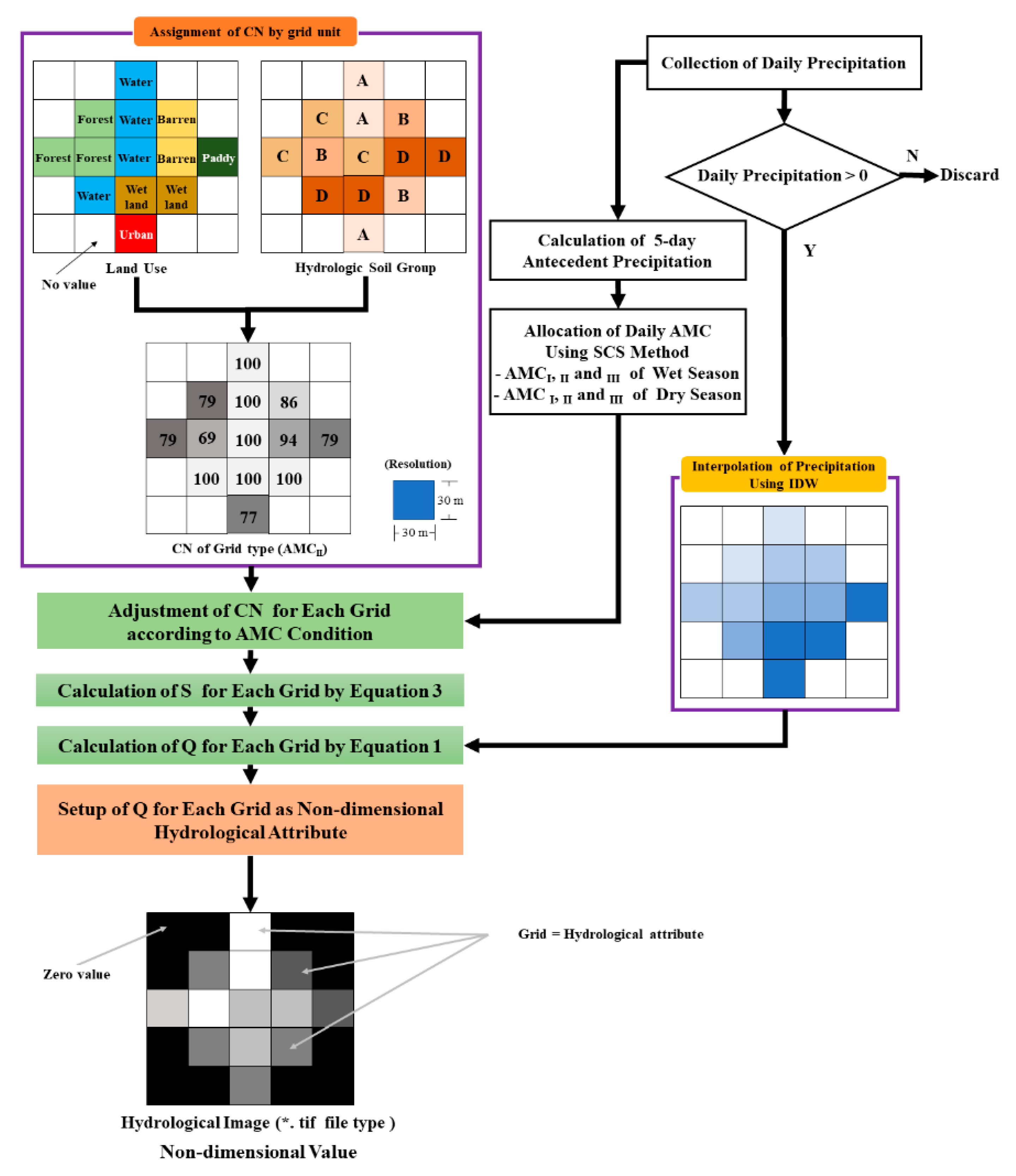
The hydrological properties of each grid point in the image was based on the hydrological curve number (CN) [29], as shown in Equations (1)–(3), published by the SCS, formerly known as the National Resource Conservation Service. The CN is a value derived using conditions such as precipitation, soil map, and land use, and it is used to simulate direct runoff (mm), as well as for evaluating hydrological effects such as direct runoff caused by land-use change [30,31].
where Q denotes the amount of direct runoff (mm), P is the amount of precipitation (mm), Ia means the initial loss (mm), and S is the amount of residual storage (mm).
The CN in Equation (3) was allocated according to the physical properties and land use of the four soils divided into hydrologic soil groups (HSGs) A, B, C, and D. In South Korea, this method can be used as it is. However, the estimated discharge had an enormous error because the proposed CN in the SCS was built using the result of an experiment in United States (US) terrain. Consequently, South Korea re-manufactured the CN for the topographic conditions of South Korea. For this reason, the CN proposed in the Design Flood Estimation Techniques [32] by the Ministry of Land, Transport, and Maritime Affairs of South Korea was used in this study. The hydrological properties of each grid to generate hydrological images were calculated using Equations (1)–(3) proposed by the SCS, where Q in Equations (1) and (2) is the proxy of hydrological property [29].
The Thiessen polygon method [33] was proposed as a method of based on measurements of precipitation. However, this method has a disadvantage of generating distortions or differences in precipitation due to the discontinuity of numerical change at the polygonal boundary. Moreover, if the same precipitation is applied to calculate the hydrological properties for each grid as done herein, the hydrological image becomes very monotonous, making it unsuitable as training data for the CNN model. In this study, two-dimensional data of precipitation in grid units were constructed using inverse distance weighting (IDW) without using the Thiessen polygon method. As IDW is an interpolation method based on Tobler’s law [34], it can estimate continuous precipitation change in grid units, thereby compensating for the disadvantages of the Thiessen polygons. In addition, the SCS proposed a modification of CN [29] considering the effect of precipitation in order to take into account the change in runoff due to antecedent precipitation. SCS introduced the concept of antecedent moisture condition (AMC), which is the cumulative precipitation for 5 days, and proposed dividing it into three stages—AMCI, II, and III—according to the dry and wet seasons. Moreover, the CN in Equation (3) represents the AMCII condition. Through this, the SCS proposed that CN can be adjusted according to conditions such as AMC changes, as shown in Equations (4) and (5). This adjustment was done and reflected in the calculation of the hydrological properties of each grid. However, in terms of the dry and wet seasons, the dry season was classified as from October to May and the wet season was classified as from June to September according to the climatic characteristics of South Korea, where precipitation is concentrated from June to September (Table 2).
where CNI is the CN for the AMCI condition and CNIII is the CN for the AMCIII condition.
As the image of the non-precipitation condition was fixed, the data were excluded from the dataset composition, and only the data in the event of precipitation were collected. The collected data were converted into a TIF format file, an image file format that has the same two-dimensional structure as the land-use and soil map to be constructed as a feature. The TIF format file was used as the runoff data, which is the property value of the grid, and it was converted into meaningful color values in the integer range of 0–255, resulting in information loss if formats such as JPG, BMG, and PNG were used.
Consequently, the building process was as shown in Figure 3. Hydrological attributes were calculated using the CN value and precipitation value of each grid. The bottom grid plot of the Figure 3 corresponds to the final hydrological image. The grid color becomes whiter as the grid value increases and becomes darker as the grid value decreases. Here, the hydrological images were built using Python 3.7 which is an open-source language.
- (2)
- Target Data
In this study, three discharge data corresponding to the entire study area—JJ, HC, and BH—were used as target data that were subsequently built into a CSV format file to be recognized by the CNN model. The target data were for supervised training of the CNN model, and the CNN model herein was trained using hydrological images. The error was calculated through the difference between the estimated value derived on this basis and the target data, and the process of reducing the error through training was iterated. In this study, the target data were the discharge data corresponding to the date of the hydrological image.
- (3)
- Dataset Setting
The previously built hydrological image and target data were used as a dataset for the prediction and training of the CNN model. Basically, the dataset was divided into an input dataset and a test dataset. The input dataset was divided into a training dataset for model training and a validation dataset for verification of model training. As a method of setting the dataset, the datasets corresponding to two watersheds were used to train the model and the datasets corresponding to one watershed were used to examine the prediction performance of the model. The datasets of the three cases were set as shown in Table 3.
2.3.2. CNN Structure Configuration
The development of the CNN algorithm was accelerated by LeCun et al. [35], mimicking the visual processing of object recognition in organisms. CNN has been applied to image classification, speech recognition, and image semantic segmentation [36]; CNN has also been very quickly evaluated as a core technology in the image classification field owing to its advantages such as reliable results and outstanding efficiency [37,38,39]. CNN can process two-dimensional or three-dimensional input data instead of the one-dimensional input data used in the conventional ANN. In particular, it learns the spatial information of the input data and can efficiently understand spatial attributes. The CNN model can be mainly divided into two parts. Part 1 comprises repetition of the convolution layer and the pulling layer, and Part 2 comprises a flatten layer, a dense layer, and an output layer in a fully connected layer connected after Part 1.
Part 1 is the core function of CNN that maintains the shape of the input/output data of each layer and spatial data of the image while effectively recognizing the attribute of the adjacent images. The convolution layer of Part 1 performs extraction of the image’s characteristics by using the image searching window called the kernel while maintaining the shape of the image. Figure 4a shows the scheme of the convolution layer. The kernel moves on the input image and makes a new image of a different size from the input image. This image is called the feature, and the size of the feature depends on the kernel’s moving distance, which is called the stride. The kernel acts like a weighted value in the ANN and is optimized by the CNN model training. The pooling layer reduces the size of the feature by down-sampling and has the function of inhibiting overfitting. Since the pooling layer also has a kernel and a stride, the size of the feature changes when the feature passes through the pooling layer (Figure 4b).
Part 2 refers to a DNN composed of several hidden layers or dense layers between the flatten layer and the output layer that derives the simulation results [40,41]. Figure 4c shows the flatten layer and the dense layer of Part 2. The flatten layer has the function of converting features into one-dimensional data as shown in Figure 4c. Furthermore, the dense layer in Figure 4c is the same as the hidden layer in ANN, where each dense layer is optimized by updating the weight of each node in dense layer.
As mentioned above, as the CNN model was operated for the purpose of solving the classification issue, the current CNN model is unsuitable for simulating unspecified continuous variables such as discharge rate. Therefore, the CNN model was improved herein as shown in Figure 5. Part 1 was designed in a structure wherein the convolution layer and the pulling layer are repeated five times, and Part 2 was designed in a structure wherein a flatten layer, two density layers, and a batch normalization layer are arranged, and a density layer is re-connected. Here, the batch normalization layer is characterized by improving the gradient vanishing and local minima, enabling stable model training [42].
The CNN model uses the Softmax or Sigmoid function as the activation function to solve classification problems. However, a linear function has frequently been used in the regression model instead of the Softmax or Sigmoid function. Because this paper aimed to simulate the discharge, the activation function in the last dense layer of this CNN model was set as a linear function. Keras [43], which uses the function of Tensorflow [44] (a machine training library released by Google), was used as the environment for CNN model design, implementation, and operation, which was subsequently implemented and experimented in Python. Keras is a high-level DNN application programming interface written in Python that supports all special functions of Tensorflow and has very high flexibility in implementing DNN models. In addition, fast experiments can be conducted as it can efficiently use the central and graphics processing units (CPU and GPU) [43].
2.3.3. Detailed Modified Configuration
CNN uses a separate 2D plane function called a kernel, a type of image filter, which is in the convolution layer and plays the role of a parameter to obtain the image features. The size of the kernel is defined in a square shape, wherein the size and number can be arbitrarily set. In this study, all kernels were set to a size of 3 × 3, and the number of kernels was set to 32, 64, 128, 256, and 512 in the order of five convolution layers. In addition, this kernel extracted image features while searching the input image. The interval of this movement is called the stride, which was set to move by one space. The image was reduced while extracting the image features via the kernel, and the method to prevent this is called padding. Padding was also set herein to prevent information loss of output data. A rectified linear unit (ReLu) function was set as the convolution layer had an activation function as shown in Equation (6). The ReLu function is commonly used in CNN models. It can avoid gradient vanishing, and the optimization efficiency of the model is high [45,46].
The pooling layer is a sub-sampling method wherein only important information is left while reducing the size of the data received from the convolution layer as input data. It has an effect of preventing overfitting as the computer memory can be efficiently used and the calculated data are reduced. There are max pooling and average pooling methods for pooling. Max pooling was used in this model as average pooling can cause loss of information. The size of the pooling can also be arbitrarily set. In this study, the size of the convolution layer was set to 3 × 3 as the kernel size. The neural network using supervised training optimizes the model by continuously updating the parameters to minimize errors between the predicted values and target values of the model derived during training. The error is called loss in neural networks, and the purpose of supervised training can be described as minimizing loss. The change in loss can be used as an index to determine the result of model training, and the change in loss can be monitored using the loss function. Mainly, the CNN model uses loss functions such as binary cross-entropy, categorical cross-entropy, and sparse categorical cross-entropy. These are loss functions for the purpose of classification and are unsuitable for a model predicting continuous variables as done herein. Therefore, mean square error (MSE), which is widely used in regression problems, was used as the loss function in this study, as shown in Equation (7), and the training degree (optimization) of the model was determined on this basis. The item to be examined together with model training was the predictive performance of the trained model. As an examination metric, the mean absolute error (MAE) was applied herein, as shown in Equation (8).
where and denote a measured value and a predicted value, respectively. In addition, as MSE and MAE converge to 0, the performance of the model can be considered to be higher. Even if the result of the loss function and the predictive performance of the model are moderate or good, it is the result of training between the input data and the target data for model training. Therefore, it should be verified that smooth prediction is derived even for new data (or unseen data) not used in model training. This is also called model generalization. In this study, some of the collected data were selected as a validation dataset to evaluate the generalization of the model. The results of model training were determined using loss, MAE, validation loss (Val loss), and validation MAE (Val MAE), where loss and MAE refer to training indices for input data, and Val loss and Val MAE refer to validation indices in the validation dataset. In terms of the algorithm for optimization, the stochastic gradient descent (SGD) [47] was considered to be the most basic methodology. Whenever the weight is updated, the SGD measures the slope through differentiation and subsequently updates toward a lower slope to reduce loss. To improve the shortcomings of SGD in recent years, optimization algorithms such as Momentum [48], Nesterov Accelerated Gradient [49], Adagrad [50], Nadam [51], AdaDelta [52], RMSProp [53], and Adam [54] were used to improve training speed and accuracy based on SGD. Adam, referring to adaptive momentum estimation, is a combination of the concepts of momentum optimization and RMSProp, which follows the exponential decaying average of the gradient similar to momentum optimization and follows the exponential decaying average of the square of the last gradient similar to RMSProp [55]. Adam with these characteristics has a function enabling stable and fast optimization of the model, leading to better results than other optimization methods. Adam was herein set as the weight optimization algorithm of the model, whereby the learning rate was set to 0.0001 and the training epoch was set to 500. The CNN model training herein was performed on a desktop using an Intel® Core™ i9-9900K CPU @ 3.60 GHz, 32 GB random-access memory (RAM), NDIVIA® GEFORCE RTX™ 2080Ti GPU, and Windows operating system (OS).
2.4. Evaluation of Model
For the evaluation of the model, its performance was determined by comparing the measured value and the predicted value. Three methods were used to evaluate the model: Pearson correlation coefficient (r), Nash–Sutcliffe efficiency (NSE), and root-mean-square error (RMSE); r ranged from −1 to 1 and was a method to examine the linearity relationship between the measured and predicted values. The value of r was measured as shown in Equation (9), with values closer to 1 denoting stronger linearity between the predicted value and the measured value, according to which the performance of the model was determined to be good.
The NSE is presented in Equation (10). NSE ranges from 0 to 1, with the model results being in perfect agreement when the measured values of NSE are 1. On the other hand, the model performance degrades as it converges to zero.
RMSE shows how close the model predicts to the measured value, as shown in Equation (11), and the value ranges from 0 to infinity within the range of the data. In general, RMSE follows the unit of the target to be simulated; thus, the RMSE of this study was equal to the discharge rate unit of m3/s. Although the evaluation criteria for the RMSE itself are not clear, a closer value to 0 denotes that the model results are closer to the measured values.
where and denote the measured values and predicted values, respectively, while and present the average measured values and predicted values.
3. Result and Discussion
3.1. Precipitation and Discharge by Watershed
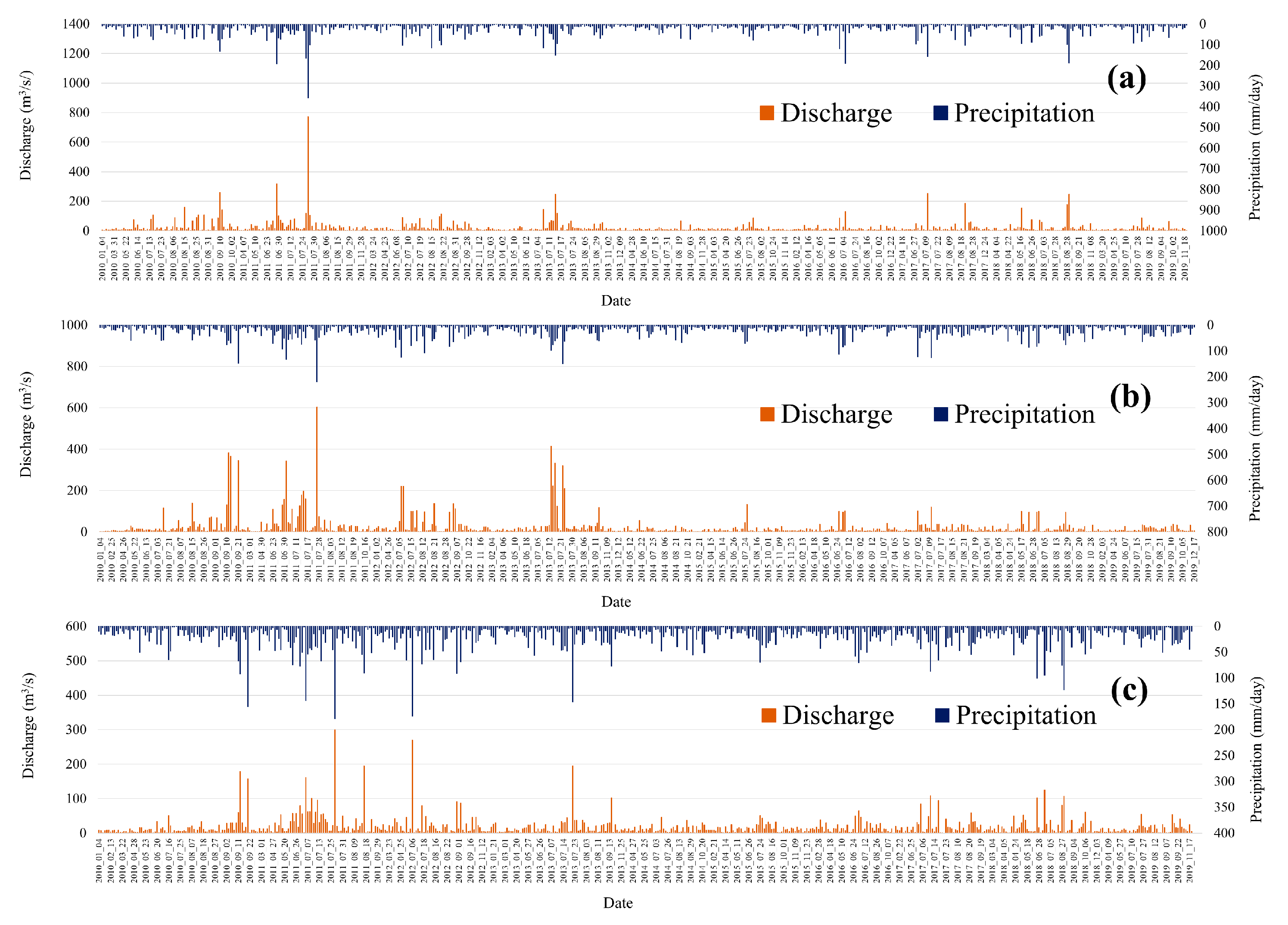
The number of precipitation events in the period of 10 years from 2010 to 2019 during the study period was 566, 571, and 554 for JJ, HC and BH, respectively. For JJ, the precipitation range was 0.5–358.0 mm, and the range of discharge was 0.8–774.0 m3/s (Figure 6a). For HC, the precipitation range was 0.3–218.6 mm, and the range of discharge was 0.2–603.2 m3/s (Figure 6b). For BH, the precipitation was 0.5–178.8 mm, and the range of discharge was 0.9–299.5 m3/s (Figure 6c). All three watersheds showed the highest discharge rate in 2011, possibly due to the highest precipitation in 2011 (1.581.6 mm) compared to other years. In addition, the average value of discharge was 18.5 m3/s for BH, 25.5 m3/s for HC, and 23.1 m3/s for JJ, which is considered to be the effect of the watershed area as shown in Table 1.
3.2. Result of Building the Hydrological Image
As explained in Section 3.1, the number of hydrological images was 554 for JJ, 571 for HC, and 566 for BH, like the number of days of precipitation in the three study areas. Figure 7 shows one of the three hydrological images of the study areas. All hydrological images of all study areas were built according to equations 1–3 using a 30 m × 30 m resolution Precipitation Image and CN Image. JJ, HC and BH were images with grids of 670 × 819, 1014 × 632 and 513 × 872, respectively. The CNN model is required to have the same size for all input data images. Hence, they cannot be used for CNN model training as each study area had a different size as shown in Figure 7b. Therefore, the hydrological images of all study areas were rebuilt to 1014 × 1014 herein based on 1014, which is the largest size of the study area as shown in Figure 7c. In terms of the method, Pillow’s linear interpolation method [56], an image module of Python, was used in this study.
Although the readjusted hydrological images were used for the training and testing of the CNN model and the data were used for training, verification, and testing of the model, there is no standard set for the data ratio. However, training and verification data were used in the ratio of 7:3 or 8:2 in several previous studies [57,58,59,60]. Therefore, the data were divided as shown in Table 4, and the model was divided into Cases 1, 2, and 3, used herein for training, verification, and testing, respectively.
3.3. Model Structure and Training Results
The CNN model used herein is as shown in Table 5. As designed, it comprised a structure wherein the convolution layer and the pooling layer were repeated five times with a structure followed by a fully connected layer. The total number of parameters, which is the number of weights in the CNN model, was 27,850,241, the number of trainable parameters was 27,849,985, and the number of nontrainable parameters was 256, as shown in Table 5. The nontrainable parameters are shown due to the batch normalization layer having 285 nodes. For the purpose of this study, only one value was allowed to be the output from the last layer, i.e., dense layer 4 of Table 5, and a linear function was set as the activation function to simulate unspecified continuous variables.
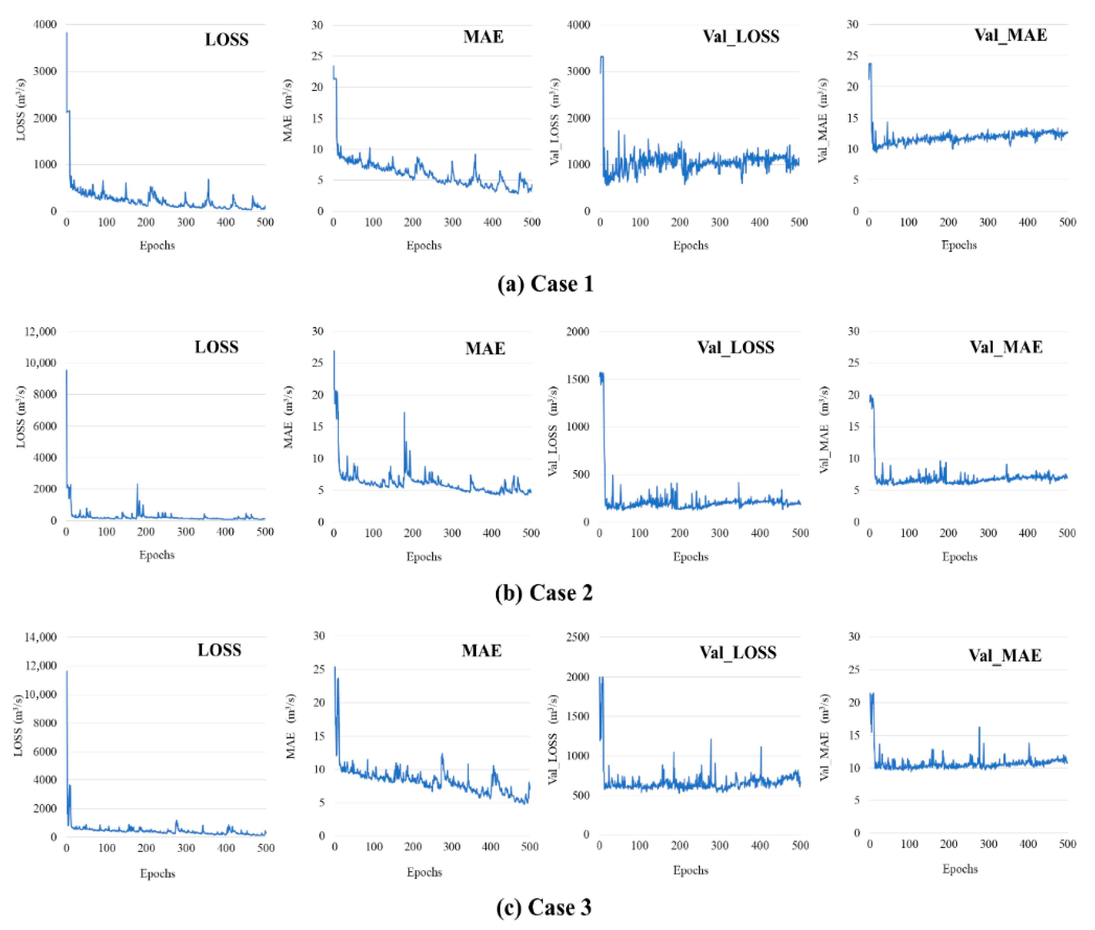
Figure 8 shows the CNN model training results of our study. Loss, MAE, Val loss, and Val MAE decreased in all three study areas. Loss in JJ reduced from 3.824.9 m3/s to 28.1 m3/s, and MAE reduced from 23.4 m3/s to 2.9 m3/s. Loss in Val reduced from 3.314.0 m3/s to 555.1 m3/s, and MAE in Val reduced from 23.7 m3/s to 9.0 m3/s (Figure 8a). Loss in HC reduced from 9.529.1 m3/s to 70.6 m3/s, and MAE reduced from 27.0 m3/s to 4.2 m3/s. Loss in Val reduced from 1.570.8 m3/s to 124.5 m3/s, and MAE in Val reduced from 20.0 m3/s to 5.8 m3/s (Figure 8b). In addition, the loss in BH reduced from 11.629.8 m3/s to 118.6 m3/s, and MAE reduced from 25.4 m3/s to 4.7 m3/s. Loss in Val reduced from 1.997.9 m3/s to 527.9 m3/s, and MAE in Val reduced from 21.5 m3/s to 9.4 m3/s (Figure 8c). Loss, MAE, Val loss, and Val MAE were referred to for determining the model training results. As mentioned above, loss and MAE refer to the training of the model for input data, and Val loss and Val MAE refer to metrics representing the degree of generalization of the model. All metrics appear as an exponential function graph with a base of 0 or less as the epoch progresses when the model is stably trained. However, the degree of training of the CNN model herein rapidly decreased at the beginning of training as shown in Figure 8. Loss and MAE should also be stably reduced, but high performance of the model can be guaranteed if the Val loss and Val MAE representing the generalization of the model are sufficiently reduced. However, as there is no clear criterion for decision, it was herein determined that both model training and model generalization were in progress as all metrics decreased with the epoch progression.
3.4. Model Prediction Results and Model Evaluation
3.4.1. Model Prediction
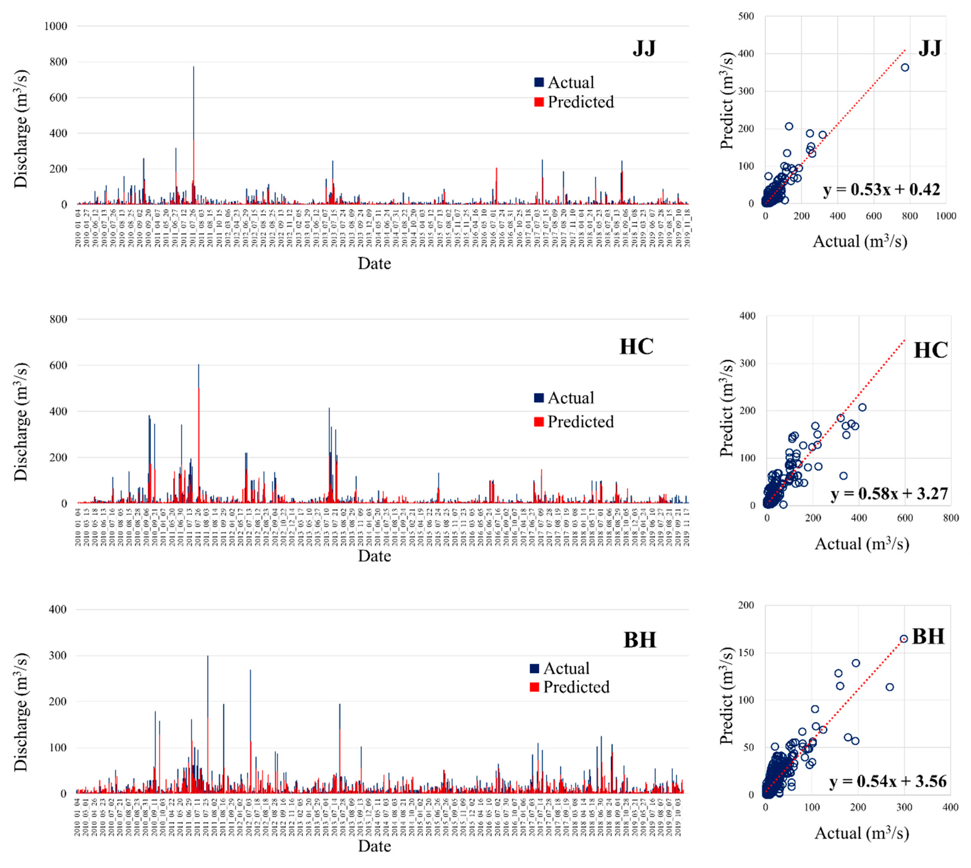
Using the classified data in Table 5 and Cases 1–3 of the model for estimating the discharge in the ungauged watershed, the prediction results of the precipitation for the entire study period are shown in Figure 9. The result of simulating the discharge of JJ using the Case 1 model, the discharge of HC using the Case 2 model, and the discharge of BH using the Case 3 model are shown in Figure 9a–c, respectively. The measured and predicted values of the discharge are as shown on the left graph in Figure 9a–c and the distribution of the measured versus predicted values is as shown on the right graph. The predicted value in Cases 1–3 tended to show a lower value than the actual value, and this can also be seen on the graphs to the right where the slope is much less than 1. However, it followed the measured value overall. In the case of the dispersion, a linear relationship between the measured value and the predicted value was shown in all models.
3.4.2. Model Evaluation
To evaluate this model, Equations (9)–(11) were used to determine r, NSE, and RMSE, as shown in Table 6. In general, when evaluating the model using r, it was seen as weak when the value of r was in the range of 0.1–0.3, as moderate in the range of 0.4–0.6, as strong in the range of 0.7–0.9, and as perfect when it was 1 [61]. When evaluating the model using NSE, it was seen as moderate if the value of NSE was in the range of 0.6–0.8 and as good if it was above 0.8 [62]. In this model, r of Cases 1–3 was 0.9, showing a strong correlation, and NSE of Cases 1–3 was 0.7, indicating that all cases were moderate. In terms of the RMSE, Case 3 was 16.1 m3/s, Case 1 was 27 m3/s, and Case 2 was 28.5 m3/s, indicating that the RMSE in Case 1 was the lowest. These results determined that the discharge simulation methodology of ungauged watershed using hydrological images and that the CNN model has moderate predictive performance overall. Case 3 had a singular point unlike other cases. The BH simulated by Case 3 showed moderate discharge prediction results similar to Cases 1 and 2, which are forest-dominant areas, even though it had more agricultural areas than forest areas compared to other study areas. This model reflected the land use of the study area through hydrological images.
This study tried to compare the results of this paper and similar papers. This was difficult because few studies were conducted on the discharge simulation of an ungauged watershed using the CNN model. Instead, this paper compared results with a previous paper using the ANN model. The CNN model using a hydrological image with spatial attribute could derive moderate results for the discharge simulation of the ungauged watershed, and the hydrological image had sufficient utility as input data for the CNN model. In addition, considering the aspect of not using the watershed data for CNN model training to simulate the discharge of ungauged watersheds, our CNN model had sufficient function as a discharge prediction model for ungauged watersheds. However, the prediction results such as the RMSE of this model were observed to be similar or lower than the results of the preceding studies mentioned in Section 1. Therefore, even if r or NSE showed moderate results, this model has limitations in terms of quantitative numerical prediction. This was attributable to the structure of the CNN model used herein designed in a relatively simple structure, and the data used depend only on hydrological images, whereby the number of images was extremely small as mentioned earlier. However, our study is meaningful in that a new methodology for estimating the discharge rate in the ungauged watershed was proposed by developing a CNN model using hydrological images, and moderate results were derived.
4. Conclusions
The CNN model is a neural network model developed to solve the classification issue; however, it is unsuitable for simulating continuous variables such as discharge rate estimation. Therefore, we improved the CNN model to simulate a continuous variable by adjusting the structure of the fully connected layer while maintaining the function of the convolution layer. In addition, a hydrological image instead of a simple RGB photograph was used as the input data of the CNN model. The discharge estimation of the ungauged watershed was performed on this basis; accordingly, the prediction performance of the model was shown to be moderate. Likewise, a new methodology for estimating the discharge in the ungauged watershed was proposed herein, and the results showed that the discharge in the ungauged watershed can be estimated through a simple model. Furthermore, this model reflected the land use of the study area through hydrological images.
However, this study could not determine if the CNN model predicted the discharge using some spatial characteristic of the hydrological image. For an improvement of this limitation, the manner in which this CNN model recognizes the attributes of land use in the study area through hydrological images will be investigated in future studies. Moreover, the accuracy of the quantitative model prediction was low owing to the use of only hydrological images as input data, unlike previous studies that used the input data of several items, and the simplicity of the CNN model structure. In addition, this study had a limitation in terms of the lag time, because this study could only present a result for the event. The lag time is an important factor associated with estimating discharge. In this regard, we would like to overcome the limitations of this study by improving the lag-time problem or by improving the hydrological image.
Nevertheless, if the CNN model structure is expanded and the hydrological image is improved, or if a new image is developed using the methodology presented throughout this study, there is room for improvement in the prediction performance of the model. The CNN model is expected to be applicable to the field of remote sensing or the field of real-time discharge simulation in a global or wide area using satellite imagery. In particular, the technology for discharge estimation using the CNN model is considered to be in its infancy. However, it is believed that not only a higher model performance can be derived but also its application range can be greatly expanded considering the speed of technological development of the current CNN algorithm.
Author Contributions
Conceptualization, C.M.S.; methodology, C.M.S.; software, C.M.S. and D.Y.K.; validation, C.M.S.; formal analysis, C.M.S. and D.Y.K.; investigation, C.M.S. and D.Y.K.; resources, C.M.S. and D.Y.K.; data curation, C.M.S. and D.Y.K.; writing—original draft preparation, C.M.S. and D.Y.K.; writing—review and editing, C.M.S. and D.Y.K.; visualization, C.M.S. and D.Y.K.; supervision, C.M.S.; project administration, C.M.S. All authors have read and agreed to the published version of the manuscript.
Funding
This research received no external funding.
Conflicts of Interest
The authors declare no conflict of interest.
References
- Biswas, A.K. Integrated water resources management: A reassessment. Water Int. 2004, 29, 248–256. [Google Scholar] [CrossRef]
- Environmental Protection Agency (US-EPA). Guidelines for Reviewing TMDLs under Existing Regulations; US-EPA: Washington, DC, USA, 2002. Available online: https://www.epa.gov/sites/production/files/2015-10/documents/2002_06_04_tmdl_guidance_final52002.pdf (accessed on 5 November 2019).
- Duan, Q.; Sorooshian, S.; Gupta, V.K. Optimal use of the SCE-UA global optimization method for calibrating watershed models. J. Hydrol. 1994, 158, 265–284. [Google Scholar] [CrossRef]
- United States Department of Agriculture, Soil Conservation Service (USDA-SCS). Chapter 10: Estimation of Direct Runoff from Storm Rainfall. In National Engineering Handbook Hydrology Chapters; USDA-SCS: Washington, DC, USA, 2004. [Google Scholar]
- Sivapalan, M.; Takeuchi, K.; Franks, S.W.; Gupta, V.K.; Karambiri, H.; Lakshmi, V.; Liang, X.; McDonnell, J.J.; Mendiondo, E.M.; O’Connell, P.E.; et al. IAHS decade on Predictions in Ungauged Basins (PUB), 2003–2012: Shaping an exciting future for the hydrological sciences. Hydrol. Sci. J. 2003, 48, 857–880. [Google Scholar] [CrossRef] [Green Version]
- US Army Corps of Engineers Hydrologic Engineering Center. HEC-RAS 2D Modeling User’s Manual; USACE: Davis, CA, USA, 2016; Available online: https://www.hec.usace.army.mil/software/hec-ras/documentation/HEC-RAS%205.0%202D%20Modeling%20Users%20Manual.pdf (accessed on 5 February 2020).
- Mastin, M.C.; Thanh, L. User’s Guide to SSARRMENU.; US Geological Survey: Tacoma, WA, USA, 2002. Available online: https://pubs.usgs.gov/of/2001/ofr01439/pdf/ofr01-439.pdf (accessed on 5 February 2020).
- Lewis, A.R. Storm Water Management Model. User’s Manual; Water Supply and Water Resources Division National Risk Management Research Laboratory: Cincinnati, OH, USA, 2004. Available online: https://www.epa.gov/sites/production/files/2019-02/documents/epaswmm5_1_manual_master_8-2-15.pdf (accessed on 12 September 2020).
- Nourani, V.; Komasi, M.; Alami, M.T.; Aalami, M.T. Hybrid wavelet-genetic programming approach to optimize ANN modeling of rainfall-runoff process. J. Hydrol. Eng. 2012, 17, 724–741. [Google Scholar] [CrossRef]
- Duan, Q.; Sorooshian, S.; Gupta, V. Effective and efficient global optimization for conceptual rainfall-runoff models. Water Resour. Res. 1992, 28, 1015–1031. [Google Scholar] [CrossRef]
- Cheng, C.; Ou, C.; Chau, K. Combining a fuzzy optimal model with a genetic algorithm to solve multi-objective rainfall–runoff model calibration. J. Hydrol. 2002, 268, 72–86. [Google Scholar] [CrossRef] [Green Version]
- Chen, Y.; Li, J.; Xu, H. Improving flood forecasting capability of physically based distributed hydrological models by parameter optimization. Hydrol. Earth Syst. Sci. 2016, 20, 375–392. [Google Scholar] [CrossRef] [Green Version]
- Huo, J.; Zhang, Y.; Luo, L.; Long, Y.; He, Z.; Liu, L. Model parameter optimization method research in heihe river open modeling environment (HOME). Int. J. Pattern Recognit. Artif. Intell. 2017, 31, 1759017. [Google Scholar] [CrossRef]
- Maier, H.R.; Jain, A.; Dandy, G.C.; Sudheer, K. Methods used for the development of neural networks for the prediction of water resource variables in river systems: Current status and future directions. Environ. Model. Softw. 2010, 25, 891–909. [Google Scholar] [CrossRef]
- Patel, A.B.; Joshi, G.S. Modeling of rainfall-runoff correlations using artificial neural network—A case study of Dharoi watershed of a Sabarmati River Basin, India. Civ. Eng. J. 2017, 3, 78–87. [Google Scholar] [CrossRef]
- Salas, F.R.; Somos-Valenzuela, M.A.; Dugger, A.; Maidment, D.R.; Gochis, D.J.; David, C.; Yu, W.; Ding, D.; Clark, E.P.; Noman, N. Towards real-time continental scale streamflow simulation in continuous and discrete space. J. Am. Water Resour. Assoc. 2018, 54, 7–27. [Google Scholar] [CrossRef]
- Akhtar, M.K.; Corzo, G.A.; Van Andel, S.J.; Jonoski, A. River flow forecasting with artificial neural networks using satellite observed precipitation pre-processed with flow length and travel time information: Case study of the Ganges river basin. Hydrol. Earth Syst. Sci. 2009, 13, 1607–1618. [Google Scholar] [CrossRef] [Green Version]
- Dahl, G.E.; Sainath, T.N.; Hinton, G.E. Improving deep neural networks for LVCSR using rectified linear units and dropout. In Proceedings of the 2013 IEEE International Conference on Acoustics, Speech and Signal Processing, Vancouver, BC, Canada, 26–31 May 2013; Institute of Electrical and Electronics Engineers (IEEE): New York, NY, USA, 2013; pp. 8609–8613. [Google Scholar]
- Deng, L.; Hinton, G.; Kingsbury, B. New types of deep neural network learning for speech recognition and related applications: An overview. In Proceedings of the 2013 IEEE International Conference on Acoustics, Speech and Signal Processing, Vancouver, BC, Canada, 26–31 May 2013; Institute of Electrical and Electronics Engineers (IEEE): New York, NY, USA, 2013; pp. 8599–8603. [Google Scholar]
- Seckin, N. Modeling flood discharge at ungauged sites across Turkey using neuro-fuzzy and neural networks. J. Hydroinformatics 2010, 13, 842–849. [Google Scholar] [CrossRef]
- Maca, P.; Pech, P.; Pavlásek, J. Comparing the selected transfer functions and local optimization methods for neural network flood runoff forecast. Math. Probl. Eng. 2014, 2014, 782351. [Google Scholar] [CrossRef] [Green Version]
- Kumar, P.; Praveen, T.V.; Prasad, M.A. Artificial neural network model for rainfall-runoff-A case study. Int. J. Hybrid. Inf. Technol. 2016, 9, 263–272. [Google Scholar] [CrossRef]
- Kashani, M.H.; Ghorbani, M.A.; Dinpashoh, Y.; Shahmorad, S. Integration of Volterra model with artificial neural networks for rainfall-runoff simulation in forested catchment of northern Iran. J. Hydrol. 2016, 540, 340–354. [Google Scholar] [CrossRef]
- Kimura, N.; Yoshinaga, I.; Sekijima, K.; Azechi, I.; Baba, D. Convolutional neural network coupled with a transfer-learning approach for time-series flood predictions. Water 2019, 12, 96. [Google Scholar] [CrossRef] [Green Version]
- KMA: Korea Meteorological Administration. Available online: https://www.kma.go.kr (accessed on 3 January 2020).
- WAMIS: Water Management Information System, National Institute of Environmental Research. Available online: https://www.water.nier.go.kr (accessed on 1 March 2019).
- EGIS: Environmental Geographic Information Service. Available online: https://www.egis.me.go.kr (accessed on 9 January 2019).
- Song, C.M. Hydrological image building using curve number and prediction and evaluation of runoff through convolution neural network. Water 2020, 12, 2292. [Google Scholar] [CrossRef]
- Natural Resources Conservation Service (NRCS). Urban. Hydrology for Small Watersheds; United States Department of Agriculture, Conservation Engineering Division, Natural Resources Conservation Service: Washington, DC, USA, 1986. Available online: https://www.nrcs.usda.gov/Internet/FSE_DOCUMENTS/stelprdb1044171.pdf (accessed on 20 May 2020).
- Li, C.; Liu, M.; Hu, Y.; Shi, T.; Zong, M.; Walter, T. Assessing the impact of urbanization on direct runoff using improved composite CN method in a large urban area. Int. J. Environ. Res. Public Health 2018, 15, 775. [Google Scholar] [CrossRef] [Green Version]
- Wang, H.; Chen, Y. Identifying key hydrological processes in highly urbanized watersheds for flood forecasting with a distributed hydrological model. Water 2019, 11, 1641. [Google Scholar] [CrossRef] [Green Version]
- Ministry of Land, Infrastructure and Transport, South Korea. Design Flood Estimation Techniques; Ministry of Land Transport and Maritime Affairs: Seoul, Korea, 2012. (In Korean)
- Schumann, A.H. Thiessen polygon. In Encyclopedia of Hydrology and Lakes. Encyclopedia of Earth Science; Springer: Dordrecht, Germany, 1998; pp. 648–649. Available online: https://doi.org/10.1007/1-4020-4497-6_220 (accessed on 11 March 2020).
- Miller, H. Tobler’s First Law and Spatial Analysis. Ann. Assoc. Am. Geogr. 2004, 94, 284–289. [Google Scholar] [CrossRef]
- LeCun, Y.; Bottou, L.; Bengio, Y.; Haffner, P. Gradient-based learning applied to document recognition. Proc. IEEE 1998, 86, 2278–2324. [Google Scholar] [CrossRef] [Green Version]
- Taravat, A.; Del Frate, F.; Cornaro, C.; Vergari, S. Neural networks and support vector machine algorithms for automatic cloud classification of whole-sky ground-based images. IEEE Geosci. Remote. Sens. Lett. 2014, 12, 666–670. [Google Scholar] [CrossRef]
- Yu, S.; Jia, S.; Xu, C. Convolutional neural networks for hyperspectral image classification. Neurocomputing 2017, 219, 88–98. [Google Scholar] [CrossRef]
- Li, Q.; Cai, W.; Wang, X.; Zhou, Y.; Feng, D.D.; Chen, M. Medical image classification with convolutional neural network. In Proceedings of the 2014 13th International Conference on Control Automation Robotics & Vision (ICARCV), Singapore, 10–12 December 2014; Institute of Electrical and Electronics Engineers (IEEE): New York, NY, USA, 2014; pp. 844–848. [Google Scholar]
- Hussain, M.; Bird, J.J.; Faria, D.R. A Study on CNN Transfer Learning for Image Classification. In Advances in Intelligent Systems and Computing; Springer Science and Business Media LLC: Berlin, Germany, 2019; pp. 191–202. [Google Scholar]
- Medina, E.; Petraglia, M.R.; Gomes, J.G.R.C.; Petraglia, A. Comparison of CNN and MLP classifiers for algae detection in underwater pipelines. In Proceedings of the 2017 Seventh International Conference on Image Processing Theory, Tools and Applications (IPTA), Montreal, QC, Canada, 28 November–1 December 2017; Institute of Electrical and Electronics Engineers (IEEE): New York, NY, USA, 2017; pp. 1–6. [Google Scholar]
- Zeiler, M.D.; Fergus, R. Visualizing and understanding convolutional networks. In Computer Vision-ECCV 2020; Springer Science and Business Media LLC: Berlin, Germany, 2014; Volume 8689, pp. 818–833. [Google Scholar]
- Ioffe, S.; Szegedy, C. Batch normalization: Accelerating deep network training by reducing internal covariate shift. In Proceedings of the 32nd International Conference on Machine Learning, Lille, France, 6–11 July 2015; Volume 1, pp. 448–456. [Google Scholar]
- Keras: The Python Deep Learning API. Available online: https://keras.io/ (accessed on 27 August 2020).
- TensorFlow. An End-to-End Open Source Machine Learning Platform. Available online: https://www.tensorflow.org/ (accessed on 27 August 2020).
- Ide, H.; Kurita, T. Improvement of learning for CNN with ReLU activation by sparse regularization. In Proceedings of the 2017 International Joint Conference on Neural Networks (IJCNN), Anchorage, Alaska, 14–19 May 2017; pp. 2684–2691. [Google Scholar] [CrossRef]
- Chen, Z.; Ho, P.-H. Global-connected network with generalized ReLU activation. Pattern Recognit. 2019, 96, 106961. [Google Scholar] [CrossRef]
- Bureau of Justice Assistance. Compstat: Its origins, evolution, and future in law enforcement agencies. In Proceedings of the COMPSTAT’ 2010, Paris, France, 22–27 August 2010; Springer Science and Business Media LLC: Berlin, Germany, 2010; Volume 16, pp. 177–186.
- Qian, N. On the momentum term in gradient descent learning algorithms. Neural Netw. 1999, 12, 145–151. [Google Scholar] [CrossRef]
- Nesterov, Y. A method for unconstrained convex minimization problem with the rate of convergence. Dokl. USSR 1983, 269, 543–547. Available online: https://www.semanticscholar.org/paper/A-method-for-unconstrained-convex-minimization-with-Nesterov/ed910d96802212c9e45d956adaa27d915f5d7469 (accessed on 18 April 2020).
- Duchi, J.; Hazan, E.; Singer, Y. Adaptive subgradient methods for online learning and stochastic optimization. J. Mach. Learn. Res. 2011, 12, 2121–2159. [Google Scholar]
- Dozat, T. Incorporating Nesterov Momentum into Adam; ICLR Workshop, (1), 2013–2016, 2016. Available online: https://openreview.net/pdf/OM0jvwB8jIp57ZJjtNEZ.pdf (accessed on 21 April 2020).
- Zeiler, M.D. ADADELTA: An adaptive learning rate method. arXiv 2012, arXiv:1212.5701v1. [Google Scholar]
- Hinton, G.; Tieleman, T. RMSprop Gradient Optimization; Lecture 6e of His Coursera Class. 2014. Available online: https://www.cs.toronto.edu/~{}tijmen/csc321/slides/lecture_slides_lec6.pdf (accessed on 10 February 2019).
- Kingma, D.; Ba, J. Adam: A Method for Stochastic Optimization. In Proceedings of the International Conference on Learning Representations (ICLR), Banff, AB, Canada, 14–16 April 2014. [Google Scholar]
- Géron, A. Hands-On Machine Learning with Scikit-Learn. and Tensor Flow: Concepts, Tools, and Techniques to Build. Intelligent Systems; O’Reilly Media: Sebastopol, CA, USA, 2017. [Google Scholar]
- Pillow. Available online: https://www.python-pillow.org (accessed on 10 February 2020).
- Lee, K.; Choi, C.; Shin, D.H.; Kim, H.S. Prediction of heavy rain damage using deep learning. Water 2020, 12, 1942. [Google Scholar] [CrossRef]
- Alsumaiei, A.A. Utility of artificial neural networks in modeling pan evaporation in hyper-arid climates. Water 2020, 12, 1508. [Google Scholar] [CrossRef]
- Lee, J.; Kim, C.-G.; Lee, J.E.; Kim, N.W.; Kim, H.-J. Medium-term rainfall forecasts using artificial neural networks with Monte-Carlo cross-validation and aggregation for the Han river basin, Korea. Water 2020, 12, 1743. [Google Scholar] [CrossRef]
- Mulualem, G.M.; Liou, Y.-A. Application of artificial neural networks in forecasting a standardized precipitation evapotranspiration index for the Upper Blue Nile basin. Water 2020, 12, 643. [Google Scholar] [CrossRef] [Green Version]
- Dancey, C.; Reidy, J. Statistics without Maths for Psychology, 5th ed.; Prentice Hall: Upper Saddle River, NJ, USA, 2011; p. 620. [Google Scholar]
- Lipiwattanakarn, S.; Saengsawang, S. Performance comparison of a conceptual hydrological model and a back-propagation neural network model in rainfall-runoff modeling. Eng. J. Res. Dev. 2005, 16, 35–42. [Google Scholar]
Figure 1.
Location map of the study area.

Figure 2.
Land use map of the study watershed.

Figure 3.
Schematic of building process of hydrological image.

Figure 4.
Scheme of the convolution neural network (CNN) model.

Figure 5.
Improvement of CNN model for simulation of the discharge.

Figure 6.
Precipitation and discharge data on the date of precipitation during the data collection period: (a) JJ; (b) HC; (c) BH.
Figure 6.
Precipitation and discharge data on the date of precipitation during the data collection period: (a) JJ; (b) HC; (c) BH.

Figure 7.
Reconstruction of the hydrological image and size for each study site: (a) image elements to build hydrological image, (b) the original hydrological image, and (c) a resized hydrological image.
Figure 7.
Reconstruction of the hydrological image and size for each study site: (a) image elements to build hydrological image, (b) the original hydrological image, and (c) a resized hydrological image.

Figure 8.
Training results of CNN model: (a) Case 1, (b) Case 2, and (c) Case 3.

Figure 9.
Changes and dispersion of the prediction results of the CNN model: (a) Case 1 (JJ discharge simulation), (b) Case 2 (HC discharge simulation), and (c) Case 3 (BH discharge simulation).
Figure 9.
Changes and dispersion of the prediction results of the CNN model: (a) Case 1 (JJ discharge simulation), (b) Case 2 (HC discharge simulation), and (c) Case 3 (BH discharge simulation).


Table 1.
Summary of study areas.
| Study Areas | Land Cover | |||||||||
|---|---|---|---|---|---|---|---|---|---|---|
| Water | Urban | Barren | Pasture | Forest | Paddy | Upland | Wetland | Total | ||
| JJ (Study area 1) | Area (km2) | 2.6 | 5.8 | 5.2 | 19.2 | 207.5 | 4.4 | 13.5 | 2.4 | 260.6 |
| Proportion (%) | 1.0 | 2.2 | 2.0 | 7.4 | 79.6 | 1.7 | 5.2 | 0.9 | 100.0 | |
| HC (Study area 2) | Area (km2) | 2.3 | 6.5 | 2.9 | 22.5 | 235.8 | 20.8 | 19.6 | 3.7 | 314.1 |
| Proportion (%) | 0.7 | 2.1 | 0.9 | 7.2 | 75.1 | 6.6 | 6.2 | 1.2 | 100.0 | |
| BH (Study area 3) | Area (km2) | 1.6 | 11.7 | 4.0 | 18.2 | 41.6 | 50.9 | 49.7 | 3.5 | 181.1 |
| Proportion (%) | 0.9 | 6.5 | 2.2 | 10.1 | 23.0 | 28.1 | 27.4 | 1.9 | 100.0 | |
Table 2.
Classification of antecedent soil moisture condition [29].
Table 2.
Classification of antecedent soil moisture condition [29].
| Antecedent Soil Moisture Condition (AMC) | Sum Pi (mm) | |
|---|---|---|
| Dry Season | Wet Season | |
| AMC I (Dry condition) | P5 < 12.7 | P5 < 35.6 |
| AMC II (Normal condition) | 12.7 ≤ P5 ≤ 27.9 | 35.6 ≤ P5 ≤ 53.3 |
| AMC III (Wet condition) | P5 > 27.9 | P5 > 53.3 |
Table 3.
Dataset setting.
| Model | Watershed | Dataset Classification |
|---|---|---|
| Case 1 | JJ, HC | Input dataset (training dataset, validation dataset) |
| BH | Test data | |
| Case 2 | JJ, BH | Input dataset (training dataset, validation dataset) |
| HC | Test data | |
| Case 3 | HC, BH | Input dataset (training dataset, validation dataset) |
| JJ | Test data |
Table 4.
Dataset for CNN model.
| Model | Dataset | Number of Data | Remark | |
|---|---|---|---|---|
| Case 1 | Input dataset | Training dataset | 735 | HC–BH |
| Validation dataset | 402 | HC–BH | ||
| Test dataset | Test date set | 554 | JJ (whole study period) | |
| Case 2 | Input dataset | Training dataset | 724 | JJ–BH |
| Validation dataset | 396 | JJ–BH | ||
| Test dataset | Test date set | 571 | HC (whole study period) | |
| Case 3 | Input dataset | Training dataset | 719 | HC–JJ |
| Validation dataset | 406 | HC–JJ | ||
| Test dataset | Test date set | 566 | BH (whole study period) | |
Table 5.
Summary of the study model.
| Convolution Layer | Output Shape (Row_Size, Column_Size, Image_Channel) | Parameter | Activation Function |
|---|---|---|---|
| Conv2D 1 | 507, 507, 32 | 320 | ReLu |
| MaxPooling 1 | 253, 253, 32 | 0 | |
| Conv2D 2 | 127, 127, 64 | 18,496 | ReLu |
| MaxPooling 2 | 63, 63, 64 | 0 | |
| Conv2D 3 | 63, 63, 128 | 73,856 | ReLu |
| MaxPooling 3 | 31, 31, 128 | 0 | |
| Conv2D 4 | 31, 31, 256 | 295,168 | ReLu |
| MaxPooling 4 | 15, 15, 256 | 0 | |
| Conv2D 5 | 15, 15, 512 | 1,180,160 | ReLu |
| MaxPooling_5 | 7, 7, 512 | 0 | |
| Fully connected layer | (Number of nodes) | ||
| Flatten layer | 25,088 | 0 | |
| Dense layer 1 | 1024 | 25,691,136 | ReLu |
| Dense layer 2 | 512 | 524,800 | ReLu |
| Dense layer 3 | 128 | 65,664 | ReLu |
| Batch normalization layer | 128 | 512 | ReLu |
| Dense layer 4 | 1 | 129 | Liner |
| Total parameters: 27,850,241 | |||
| Trainable parameters: 27,849,985 | |||
| Nontrainable parameters: 256 | |||
Optimizer function: RMSprop (training ratio = 1 × 10⁻⁴); loss function: mean square error (MSE; see Equation (7)); metrics: mean absolute error (MAE; see Equation (8)); epoch: 500 iterations.
Table 6.
Result of model evaluation.
| Contents | Predicted Study Area | r | NSE | RMSE (m3/s) |
|---|---|---|---|---|
| Case 1 | JJ (study area 1) | 0.9 | 0.7 | 27.0 |
| Case 2 | HC (study area 1) | 0.9 | 0.7 | 28.5 |
| Case 3 | BH (study area 1) | 0.9 | 0.7 | 16.1 |
Publisher’s Note: MDPI stays neutral with regard to jurisdictional claims in published maps and institutional affiliations. |
© 2020 by the authors. Licensee MDPI, Basel, Switzerland. This article is an open access article distributed under the terms and conditions of the Creative Commons Attribution (CC BY) license (http://creativecommons.org/licenses/by/4.0/).
Share and Cite
MDPI and ACS Style
Kim, D.Y.; Song, C.M. Developing a Discharge Estimation Model for Ungauged Watershed Using CNN and Hydrological Image. Water 2020, 12, 3534. https://doi.org/10.3390/w12123534
AMA Style
Kim DY, Song CM. Developing a Discharge Estimation Model for Ungauged Watershed Using CNN and Hydrological Image. Water. 2020; 12(12):3534. https://doi.org/10.3390/w12123534
Chicago/Turabian StyleKim, Da Ye, and Chul Min Song. 2020. "Developing a Discharge Estimation Model for Ungauged Watershed Using CNN and Hydrological Image" Water 12, no. 12: 3534. https://doi.org/10.3390/w12123534
Note that from the first issue of 2016, this journal uses article numbers instead of page numbers. See further details here.