Evaluation in Carbon Dioxide Equivalent and CHG Emissions for Water and Energy Management in Water Users Associations. A Case Study in the Southeast of Spain

Abstract

Agriculture is an activity linked to the environment and has a great influence on climate change. As more and more crops are producing in less time, agricultural production is intensified and water consumption and energy demand is increasing. Since the energy consumed is not renewable, greenhouse gases (GHG) are emitted and their concentration in the atmosphere increases. The objective of this article is to apply various methodologies for the precise quantification of the carbon dioxide equivalent (CO₂-eq) and GHG emissions in the management of irrigation water and energy in ten water user’s associations (WUAs) in the southeast of Spain. All the studied WUAs include irrigation facilities. This paper is based on obtained data in different water and energy audits during 2017. The concept of “irrigation water management” considered in the article covers the process from its extraction through management data to its transport and application to crops through irrigation systems, as well as the reception of water. The way in which water and energy is used to irrigate crops is taken into account. Moreover, the type of energy used for irrigation and at what moment energy is demanded influence the total amount of generated GHG emissions. The tariff periods for electricity and the water needs of the crops planted also has to be taken into account, as well as the economic emissions valuation.

1. Introduction

Climate change is a reality. Climate change includes both the global warming driven by human emissions of greenhouse gases and the resulting large-scale shifts in weather patterns. Human activity is accelerating the increase in global temperature due to the concentration of Greenhouse Gases (GHG) in the atmosphere. According to the United Nations, the world population has increased exponentially in recent years. In 2015, the global population was 7349 million people, and the forecasts for the years 2030, 2050 and 2100 are 8501, 9725 and 11,213 million people, respectively [1]. With this increase in population, transport, industry, energy demand and consumption in general will also increase, while the planet’s resources are limited. The depletion of natural resources is a worrying problem at the social level, as evidenced in the “United Nations Conference on Environment and Development” organized by the United Nations in Rio de Janeiro (Brazil) in 1992 [2], as well as in the “19th Special Session of the General Assembly to Review and Appraise the Implementation of Agenda 21” from 1997 [3]. In another United Nations study carried out by the International Resource Panel, it is detailed that globally between 1970 and 2017 the use of fossil fuels increased from 6000 to 15,000 million tons and biomass increased from 9000 to 24,000 million tons; between 1970 and 2010, it went from 2500 to 3900 km³ of water consumed; and between 2000 and 2010, the total area of cropland increased from 15.2 to 15.4 million km² [4].

406/2009/EC of the European Parliament and the Council, of 23 April, on the effort of Member States to reduce their GHG emissions in order to meet the commitments made by the Community until 2020, the aim is to reduce the GHG concentrations in the atmosphere 30% in 2020 compared to 1990 and 10% compared to 2005 [5]. The adaptation in Spain was (RD) 163/2014, where the carbon footprint registry, offsetting and carbon dioxide equivalent (CO₂e) absorption projects were created [6]. These rules are adopted for the contribution to reduce GHG emissions at a national level, increase the removal of carbon sinks in the national territory and facilitate, in this way, compliance with the international commitments assumed by Spain on climate change [7].

In irrigation systems, particularly in collective irrigation networks, efficient water management is required for water user associations (WUAs). The purpose of WUAs is to control excessive water and energy consumption and to achieve cost savings. Therefore, tools related to decision support systems, management of pump stations and energy management are used. Tools that permit the control and analysis of water and energy consumption in a WUA include performance indicators [8]. These tools were applied in several WUAs and similar systems (e.g., golf courses) all over the world [8,9,10]. Moreover, the use of different sources of water supply and renewal energy systems are additional tools for reducing the water and energy print foot in WUAs [11]. These technologies are able to reduce the carbon footprint, carbon dioxide equivalent (CO₂e) and GHG, and, in general, they can contribute to reduce emissions [12]. Using the periodical control of these performance indicators and technologies, the water and energy consumption of an irrigation system were determined, and, later, correcting measures to reduce water, energy and money were proposed. By comparing the measures of similar organizations or systems, gaps between the most efficient and poorly performing ones are highlighted and, by identifying the best practices, guidelines to improve performance can be established.

In relation to GHG emissions, energy types can be categorized as renewable or non-renewable [13]. Renewable energies are traditionally defined as the energy obtained from the inexhaustible resources of nature, such as biomass, solar radiation or wind, among others [14]. On the other hand, there are fossil energy sources (such as oil and its derivatives or coal), whose use generates GHG emissions that enhance the greenhouse effect and contribute to climate change [15]. The unit of measurement for GHG emissions is CO₂e. There are six GHGs found under the Kyoto Protocol to the United Nations Framework Convention on Climate Change. Each gas has a different global warming potential (GWP) (

Table 1. Global warming potential greenhouse gases.

Greenhouse Gas	Global Warming Potential
Carbon dioxide (CO2)	1
Methane (CH4)	25
Nitrous oxide (N2O)	298
Hydrofluorocarbons (HFCs)	124–14,800
Perfluorocarbons (PFCs)	7390–12,200
Sulfur hexafluoride (SF6)	22,800

) [16]. The GWP is the contribution to the greenhouse effect that a given GHG has over 100 years in proportion to CO₂. The GHG emissions of any of these six gases are transformed into CO₂e units and the total value of GHG emissions of an activity is expressed as a single CO₂e value.

CO₂ emissions are mainly due to the consumption of fossil fuels in thermal power plants, vehicles, industries, businesses and homes. CO₂ is the most significant long-lived greenhouse gas in Earth’s atmosphere. Since the industrial revolution, anthropogenic emissions—primarily from use of fossil fuels and deforestation—have rapidly increased its concentration in the atmosphere, leading to global warming. CH₄ emissions are due to enteric fermentation, manure management, landfills, coal mining, fugitive emissions from oil and natural gas and wastewater. The Earth’s atmospheric methane concentration has increased by about 150% since 1750, and it accounts for 20% of the total radiative forcing from all of the long-lived and globally mixed greenhouse gases.

N₂O emissions are due to fertilizers applied to agricultural soils, the energy sector, manure management, wastewater and the chemical industry. N₂O occurs in small amounts in the atmosphere but has been found to be a major scavenger of stratospheric ozone, with an impact comparable to that of chlorofluorocarbons (CFCs). It is estimated that 30% of the N₂O in the atmosphere is the result of human activity, chiefly agriculture and industry. Being the third most important long-lived greenhouse gas, nitrous oxide substantially contributes to global warming. HCFCs are compounds containing carbon, hydrogen, chlorine and fluorine. Industry and the scientific community view certain chemicals within this class of compounds as acceptable temporary alternatives to chlorofluorocarbons. HFCs are used primarily in refrigeration and air conditioning equipment, fire extinguishers and aerosols. HFCs have replaced the ozone-depleting CFCs and include HFC-23, HFC-32, HFC-125, HFC-134A, HFC-143A, HFC-227ea and HFC-236fa. Almost all PFC emissions are due to the production of aluminum; they include CF4, C2F6, C3F8 and C4F10. SF₆ is an extremely potent and persistent manmade greenhouse gas that is primarily utilized as an excellent electrical insulator and arc suppressant. It is inorganic, colorless, odorless, non-flammable and non-toxic. SF₆ is used in electrical equipment. SF₆ is the most potent greenhouse gas that has been evaluated, with a global warming potential of 23,900 times that of CO₂ when compared over a 100-year period. SF₆ is inert in the troposphere and stratosphere and is extremely long-lived, with an estimated atmospheric lifetime of 800–3200 years.

Great efforts have been made to determine the carbon footprint in agriculture, such as the “GHG Protocol Agriculture Guidance” [17], which is subject to a constant process of improvement. Other European projects that have developed methodologies and tools for this purpose include the “LIFE AgriClimateChange” project [18], in which the “ACCT” tool (AgriClimateChange Tool) was developed for the calculation of the carbon footprint in agriculture. Some current research has developed an exhaustive analysis of the calculation of the carbon footprint in irrigation [19]. In this case, the calculation and improvement of the water footprint and the carbon footprint was integrated.

The use of fossil fuels in agricultural production has contributed significantly to food production in recent decades. Examples of processes in food production where the use of fossil fuels has contributed the most are mechanization, fertilizer production, processing and transportation. The dependence of the food sector on fossil fuels according to the projections of the Food and Agriculture Organization of the United Nations (FAO) will increase in the coming years, since by 2050 they forecast that food production will increase by 70% to meet demand [20].

Another concern associated with agricultural production is the scarcity of water, especially in arid or semi-arid areas where agricultural activity occupies a representative area, promoting the adaptation of agriculture to the limitation of water resources. In areas where surface water resources is scarce, agriculture must be supplied from underground water bodies, which entails a considerable increase in the energy demand for water extraction. The use of pressurized irrigation systems, due to its high application efficiency, is a trend that has been imposed as an alternative to traditional gravity irrigation in these areas with scarce water resources since greater control of the volume of water applied allows considerable water savings. The application efficiency of gravity irrigation is around 65%, while irrigation using pressurized systems is between 75% (sprinkling) and 90% (trickle). However, a new threat appears which is the energy consumption of this type of pressurized systems, increasing their carbon footprint [21,22].

The energy demanded by an irrigation system can be generated by different sources. The transformation index is a numerical factor that relates the energy consumed by an activity with the amount of GHG emissions associated with its generation, e.g., kgCO₂e/kWh. Each country has a different energy endowment, a consequence of the type and quantity of power plants or generators installed in its territory. The generation mix does not remain stable over time. The generation mix of a country is the set of energy sources used to produce energy in a given time. Analyzing the variation of the electricity generation index to estimate the carbon footprint associated with water management in irrigation is a useful tool to obtain more precise results, since very general fixed transformation indices have traditionally been used, which do not conform to reality [23].

The precise estimation of the carbon footprint associated with the management of water in irrigation is essential for making decisions that help reduce it. Previously, it is necessary to answer different questions: What amount of GHG emissions are generated by the management of water in irrigation? What methodology is used to quantify this carbon footprint? What transformation indices are used [7,24,25,26,27]?

Current projections indicate that the demand for fresh water, energy and food will increase significantly in the coming decades, all under pressure from population growth, technological and economic development, diversification of diets, urbanization and climate change. According to a report by the Organization for Economic Cooperation and Development (OECD), food production is expected to increase by 60% by 2050; it is expected that world energy consumption will grow by 80%; and it estimates that total global water withdrawals will increase by 55%. In this context, the water–energy–food nexus has emerged as a comprehensive concept that seeks to describe and address the complex nature of the interrelationships among these resources, on which achieving different social, economic and environmental objectives depends. In practical terms, it presents a concept to better understand and analyze the interactions between the natural environment and human activities, and thus work towards a more coordinated management and use of natural resources at all sectors and scales. In this way, a procedure to incorporate water source information at the inventory level and evaluate the influence of that profile on the environmental impact assessment level is described in [28]. The inclusion of the water mix in the inventory level (irrigation profile) as well as in the impact assessment level (water stress index) is straightforward to apply by life cycle assessment (LCA) practitioners, resulting in a more realistic assessment of the impacts of freshwater consumption associated to crops. Its implementation allows the quantification of promoting alternative water sources in a region suffering from significant water stress as well as to improve knowledge on the environmental impact associated to freshwater consumed by one of the irrigated crops grown (e.g., Mediterranean countries). Moreover, water supply mix (WSmix) is another perspective of the water–energy nexus [29]. The relevance of including the WSmix in Life Cycle Inventory (LCI) databases for proper water-use impact assessment is demonstrated with a case study in this publication. The paper finally concludes on the need of using the regionalized WSmix in routine LCA, which is just as straightforward as the use of the regionalized electricity supply mix. Besides, the developed WSmix provided interesting insights beyond the LCA scope to support the strategic management of water sources at various scales including the global scale. This was located in the case of Spain.

Moreover, an irrigation network is a special type of water supply network. Several energy assessment methodologies for water supply systems were developed in the last years. The sensitivity of predicted irrigation-delivery performance in a case study is developed in [30]. This methodology combines a model of steady spatially-varied canal network flow with statistical models that generate possible realizations of the random hydraulic and hydrologic parameters. Another assessment methodology is included in [31]. For this purpose, a case study in Portugal was modeled. A flow-driven analysis approach, performing the analysis for multiple flow regimes was developed. The energy consumption for crop irrigation in Southeast Spain is analyzed in [32]. In this case, the most influential factor for energy consumption was the water source. In addition, deficit irrigation, precision agriculture, wastewater reuse, conveyance efficiency improvement and their combinations were evaluated. For each one, a cost-effectiveness (CE) was developed in a case study in Greece [33]. The application of a software model was used to simulate the water flows, taking into account irrigation return flows and reservoir operations in the case study located in South Korea [34]. Another case study in India is described in [35]. Here, farmers were using a partial border strip irrigation technique with supply pipe and riser. Several tools, such as telemetry and remote control, were applied in water–energy management for irrigation systems [36]. The results provide a detailed overview of these systems in Spain, characterizing WUAs in which they are installed, their technological traits, their maintenance, the problems they face in their daily operation, their current use, the factors limiting wider use and the willingness of the WUAs to continue bearing the costs to use TM/RC features in the future. The use of simultaneous simulation tools for the location of hydro power plants (HPP) and the potential energy generated were applied [37]. These tools represented a positive competitive advantage for agricultural production reducing the carbon footprint and therefore improving the sustainability of the agricultural production. Alternative tools for water and energy management for irrigation systems were used in Southern California [38]. In this case, the potential of remotely sensed data in addressing spatially distributed irrigation equity, adequacy and sustainability was studied. Moreover, the extensive network of open drains was also found to be functioning at an optimal level according to the results of two performance indicators based on the magnitude and uniformity of groundwater depth. The study of the drainage network, as a part of an irrigation system, is cited in [39]. An integrated on-farm drainage management (IFDM) system, as an effective method of treatment by successively irrigating zones with drainage water, was applied in Greece. A complementary economical study was included. In [40], Supervisory Control and Data Acquisition systems (SCADA), combined with high-frequency irrigation, are applied in the design and management of an irrigation network. These tools are used for assessing the relative flow reduction in networks under a rotation schedule. Finally, the water–energy management in irrigation reservoirs is presented in [41]. The performance of different evaporation machine learning models that were regressed on a very small dataset and for restrictive scenarios was applied in Brazil.

In this paper, two methodologies developed in current publications are applied [19], to determine GHG emissions due to irrigation water management in several WUAs, located in southeast Spain. To show the feasibility of the methodology developed, it was applied to ten case studies with different characteristics, thus evaluating the applicability of the proposed methodologies to two different scales. This paper is oriented to estimate the potential of improvement of corrective measures in water user associations. First, a description of the used methodologies for calculation of carbon footprint in WUAs is presented. Next, the results of these indicators and the methodology for data gathering are discussed. Finally, the results of the comparison between the studied WUAs are reported to demonstrate the suitability of using these values to establish the strengths and weaknesses of the installations and propose future corrective actions.

2. Materials and Methods

The information related to the energy consumption of the irrigation system was obtained from ten WUAs located in southeast Spain during 2017, and several visits with data collection in the area and interviews with technicians and managers of the irrigated area were performed. Information on monthly energy consumption was collected of each transformer, broken down into tariff periods (valley, flat and peak). The nominal energy consumption of the boreholes and the pumping station was registered. Moreover, the power and the flow supply of each pump was obtained. These data were related to the energy consumption of each entire irrigation system. The other obtained data were the potential water consumption depending on the water demands of the implanted crops. The water needs of the crops [42] were calculated from the climatic data of the Agroclimatic Information System for the Irrigation (IVIA) of the Conselleria de Agricultura from Valencian Community (Spain) [43].

Before the determination of the proposed calculations, different audits for the WUAs were developed. The methodology described by several authors [44,45,46] to improve water and energy management was used in all WUAs. This methodology permitted the determination of several descriptive indicators and water and energy use indicators from the management data and measured field data. In these audits, the management data were obtained, and the values for an annual average period were calculated. The collective irrigation networks of the WUAs all consisted of a branched network with diversions that supply water to numerous hydrants for drip irrigation. These collective irrigation systems also count with water storage systems, which are taken into account for this study. The water source can vary in the function of the WUA, with it primarily as surface water, ground water or sewage water, in some cases.

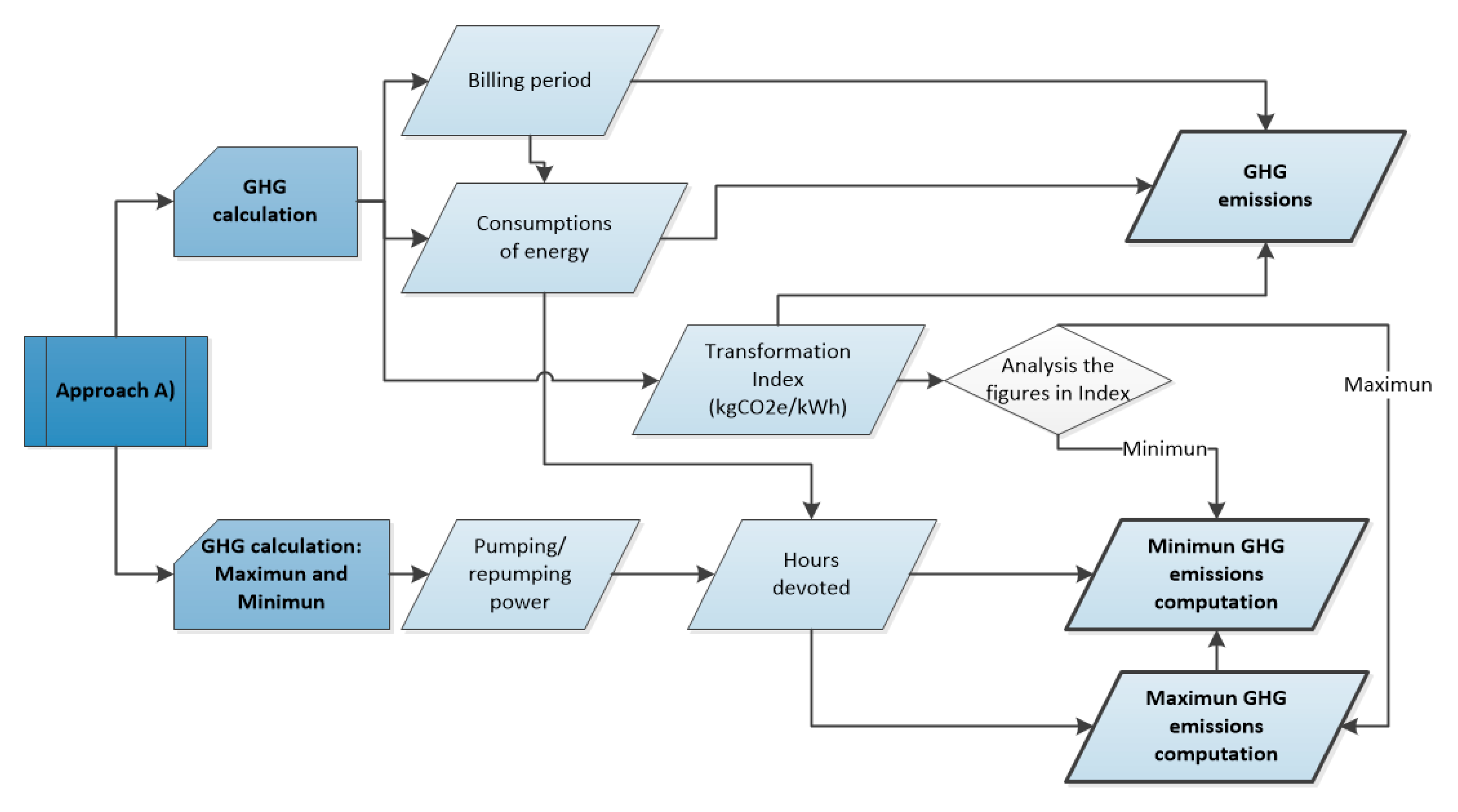
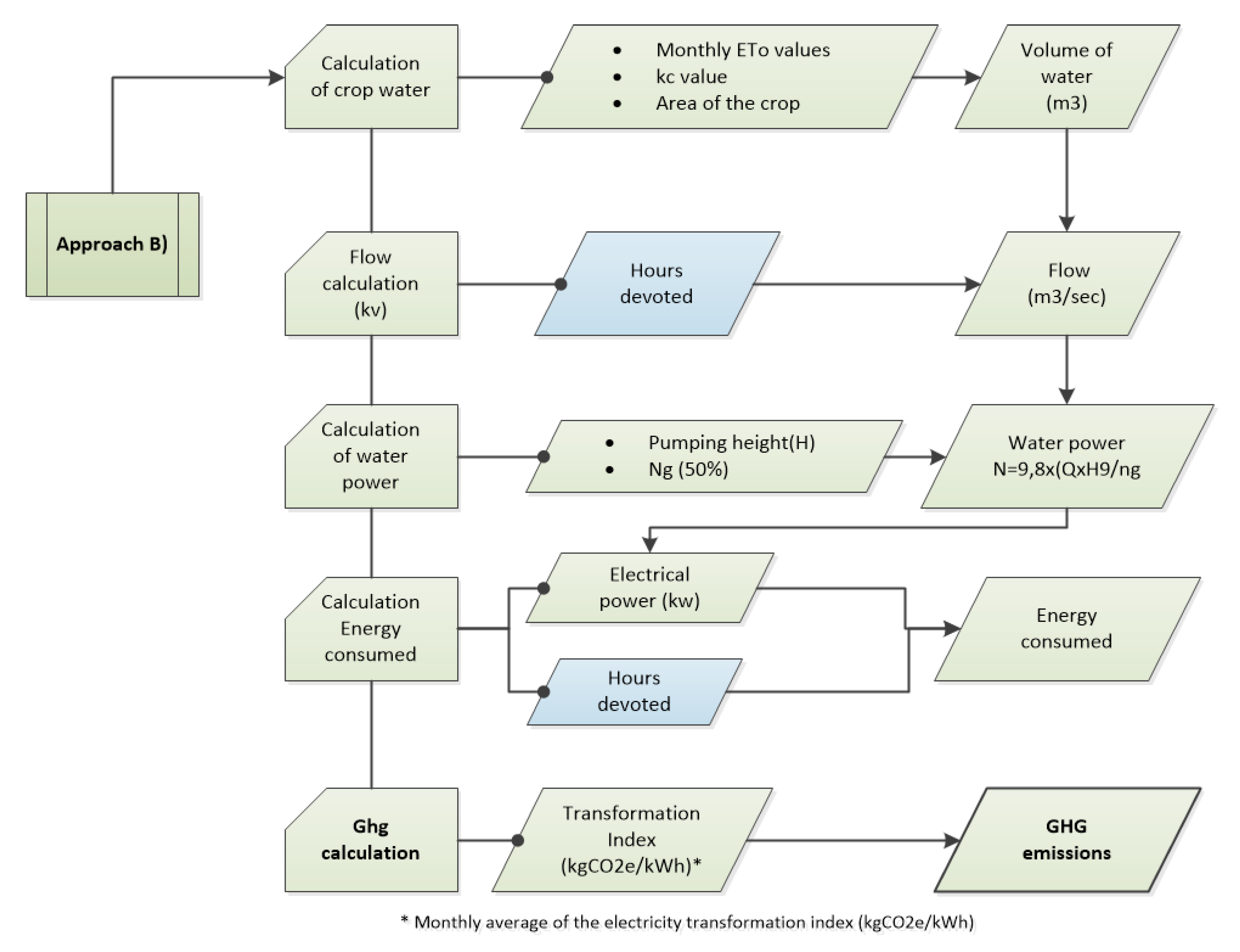
Two methodologies were proposed based on the available starting information: (1) if the electrical consumptions of the equipment involved in water management are available irrigation, Approach A was used; and (2) if there is not enough information or it is not up to date or detailed, then it is proposed to calculate GHG emissions based on the needs crop water levels (Approach B), available on the SIAR website of Spanish MAPAMA [47].

Approach A is the most accurate procedure for calculating the CO₂-eq and CHG emissions in driving of irrigation water based on measured energy consumption, since, even though irrigation recommendations come from reference public institutions such as the SIAR of the MAPAMA, they are not guaranteed to apply. Therefore, when using the energy consumption, measured uncertainty is reduced. Finally, the results of both procedures (Approaches A and B) were compared (Figure 1 and Figure 2).

For the calculation of GHG emissions through Approach A, two transformation indices were used: annual transformation index of the National Commission for Markets and Competition (in Spanish CNMC) (kgCO₂e/kWh) [48] depending on the year and monthly transformation indices, according to the tariff periods. The monthly transformation index, differentiating between tariff periods, is the best adapted to the water management of irrigation that is traditionally carried out, since it is governed mainly by the price of the energy, which is established by tariff period, which varies monthly.

In the case of the agricultural data, information was obtained on the area occupied by each cultivation in 2017. In the case of the WUAs, by having energy consumption in 2017 and without significantly modifying the distribution of crops in the set of varied surfaces of each WUA in this year, by the hypothesis of transferring energy demand, GHG emissions were calculated by applying the corresponding transformation indices and analyzing the results.

After calculating the amount of GHG emissions caused by the management of irrigation water, its economic cost was estimated. For this, we used the results of the GHG emissions estimates and the price of GHG emission rights (€/tCO₂e) that, for the analyzed year, was obtained from the website of the European CO₂ Trading System [5,25]. The average price during the studied time frame (2010–2018) was 8.85 €/tCO₂e. In 2018, it reached the maximum of this series, 15.88 €/tCO₂e. This value is practically the double of the average price. The minimum value was reached in 2013 (4.45 €/tCO₂e), a quarter of that reached in 2018. From 2018, the average price has been increasing significantly, reaching the value of 24.84 €/tCO₂e in 2019 and 23.94 €/tCO₂e in 2020 (three times the average value in 2018). The variability of the prices is answering to the different strategies and reforms in commercial relations in the energy market.

The starting data were the net needs provided by the IVIA [43].

Table 2. Characteristics of the WUAs.

WUAs	Pump Motor	Electric Meter	Power of Pump Motor (kW)	Manometric Height (m)	Irrigable Surface (he)	Crops
WUA 1					1796.78	Citrus
	1	Global	648	59.16		(100%)
	2		55	41.71
	3		162	71.73
WUA 2					778.37	Citrus
	1	Global	177	106.57		(100%)
	2		365.2
	3	Independent	90	22.39
	4	Independent	182	71.41
WUA 3					1747	Citrus (97.5%),
	1	Independent	160	52.39		Potato (1.25%),
	2	Independent	666	74.55		Artichoke (1.25%)
WUA 4					1400	Citrus,
	1	Global	566	128.74		(97.5%)
	2		41.5	21.92		Pomegranate (2.5%)
WUA 5					1130	Grape
	1	Global	150	160.50		(100%)
	2		90	60.00
WUA 6					1085	Citrus (25%),
	1	Independent	510	44.20		Potato (25%), Peach (25%), Olive (25%)
WUA 7					2000	Grape (95%);
	1	Global	496.6	91.00		Cereals (1.65%),
	2			14.30		Potatoes (1.65%),
	3			45.00		Olive (1.7%)
WUA 8					310	Citrus
	1	Independent	258.18			(100%)
	2	Independent	240
	3	Independent	45.39
	4	Independent	375
WUA 9					1730	Potato (20%),
	1	Independent	102.92	51.43		Olive (20%),
	2	Independent	140.7	171.73		Vineyard (20%)
	3	Independent	290.13	145.665		Almond tree,
	4	Independent	397.02	171.6		(20%)
	5	Independent	375.05	283.00		Peach (20%)
	6	Independent	190.77	262.79
WUA 10					593	Citrus (30%)
	1	Independent	75	35.00		Peach (20%),
	2	Independent	75	35.00		Kaki (30%)
	3	Independent	75	80.30

Global electric meter, one for all pumps; independent electric meter, one electric meter per pump. Source: Own elaboration.

shows the data related to the extension occupied by each crop on the farm. The cultivated crops in the studied WUAs were the next: citrus, potato, artichoke, pomegranate, vineyard, peach, olive grape and Persimmon [49,50,51,52,53,54,55]. Considering that the distribution of crops did not vary considerably annually, the average percentage of the total surface area occupied by each crop in 2017 is used, which was obtained from each WUA. Moreover, the characteristics of the pumping stations, number of pumps, contracted power (kW) and manometric height above the sea level, in meters, are included in Table 2.

To calculate GHG emissions related to water extraction, the volume of water to be extracted was calculated first. For this, an application efficiency of irrigation systems of 95% and an addition water extraction of 10% to compensate for evaporation losses in reservoirs and water losses in the distribution network were used [56]. The total water volume was divided between the number of boreholes, assuming each borehole draws the same amount of water.

To calculate the total hours of operation for each borehole, the energy consumed was divided for each one by the power of its engine. Irrigation scheduling is based on using the majority of the energy during the valley period (P1,

Table 3. GHG emissions (kgCO₂e) according to active and reactive power per WUAs and potential emission de emissions. Maximum and minimum GHG (Approach A).

WUAs	Active GHG			Reactive GHG	Total GHG (kgCO2e)	Min GHG (kgCO2e)	Max GHG (kgCO2e)
	P1	P2	P3
WUA 1	81,769	134,690	223,235	259,239	698,932	681,461	717,073
WUA 2	192,604	100,507	804,859	554,682	1,652,652	1,596,074	1,690,063
	189,128	78,778	608,234	381,812	1,257,952	1,216,525	1,287,801
	622	1301	8735	12,033	22,691	21,859	23,240
	2854	20,428	187,890	160,837	372,009	357,690	379,022
WUA 3	283,216	109,816	139,732	190,615	723,379	706,887	748,739
	95,234	19,217	54,671	57,546	226,668	222,292	232,092
	142,490	81,420	139,732	133,069	496,711	484,595	516,647
WUA 4	80,297	238,831	162,027	262,321	743,476	725,209	769,034
WUA 5	6256	23,252	85,170	49,584	164,262	158,752	177,133
WUA 6	12,508	26,863	28,948	11,500	79,819	77,121	84,175
WUA 7	48,323	126,936	193,860	195,037	564,156	537,027	602,113
WUA 8	27,075	51,776	58,860	48,933	186,644	182,301	192,463
	1383	3455	5703	2928	13,469	13,223	13,969
	18,448	35,438	42,279	37,563	133,728	130,690	137,982
	986	2023	2441	1414	6864	6701	7098
	6258	10,860	8437	7028	32,583	31,687	33,414
WUA 9	154,571	237,192	1,423,560	771,588	2,586,911	2,548,322	2,695,537
	1005	14,760	34,514	13,897	64,176	63,184	67,167
	87,766	105,041	304,064	241,279	738,150	722,500	767,943
	61,196	93,430	266,169	149,465	570,260	560,052	590,274
	2742	10,142	208,791	120,838	342,513	338,459	358,180
	942	8857	410,407	153,611	573,817	568,818	600,136
	920	4962	19,915	92,498	297,995	295,309	311,837
WUA 10	72,698	85,379	75,569	28,150	196,366	191,816	204,363
	895	32,382	32,795	1772	67,844	66,097	70,090
	1849	44,367	31,479	5505	83,200	81,420	86,910
	4524	8630	11,295	20,873	45,322	44,299	47,363

Source: Own elaboration. P1, peak hour; P2, flat hour; P3, valley hour.

). If it is not possible, then the flat period (P2) is used. The last option is using the peak period (P3). According to this, total operating hours were calculated for each pump and were distributed according to the irrigation schedule. Through Order ITC/3801/2008, the number of hours corresponding to each rate period was determined (assuming that each month has 4 full weeks they would be: 304 off-peak h, 248 flat h and 120 peak h). From the hours of operation in each rate period, the energy consumed, using the power of the pump motor of each borehole, and the GHG emissions generated, the monthly transformation indices were used, differentiating between tariff periods.

Once the GHG emissions related to the extraction of groundwater were determined, GHG emissions generated by the application of water to crops were calculated. To determine how much energy was consumed in each tariff period, total operating hours were calculated. To calculate the monthly operating hours of the pumping equipment, the following procedure was performed:

In the case of the agricultural exploitation, the volume of water to be applied to each crop was divided by the flow rate that the corresponding irrigation system was able to provide (drip irrigation).

In the case of the WUAs having several pumping stations with varied pumps each which start up depending on the flow rate defendant at each moment, the number of hours worked by each station at a certain power was calculated. For this, 4000 h of operation were started for each sector based on the data provided by the managers and technicians of the WUAs. This estimate was contrasted from the total volume applied to crops and the frequency of supply of flows typical of irrigation networks to the demand. It was also drawn from the data of the variable speed pump (flow, manometric head and performance). These data are relative to each sector. As each pumping station is equipped with several pumps of the same characteristics and assuming that no there are significant differences in irrigation management between sectors, the results were applied to each one.

The total hours per year (4000 h) was obtained as the average number of the WUAs and the flow frequency of the power related to each flow demanded to finally determine the number of hours associated with a given power. For this, a graph was constructed of the performance associated with the demanded flow of pumping stations, and data on the characteristics of the pumps were collected from the manufacturer (Table 2).

The powers were grouped in intervals of 50 kW. The 4000 total h were distributed monthly based on the monthly proportion of the total annual water requirements (including all crops and their extent). From the frequency associated with each flow, the hours of monthly operation of each pumping station in each power interval were calculated.

To calculate the hours of operation in each rate period, it was determined that 75% were distributed to the valley period, 20% to the flat period and 5% to the peak period, based on the estimates of the irrigation network managers and technicians.

According to Approach B, the GHG emissions are related to crop water needs. As presented in Figure 2, the final obtained value is a potential digit. The obtained value by Approach A is a measured digit, based on the use of the pumping station equipment of each WUA.

3. Results and Discussion

Table 3 shows the value of GHG emissions calculated with respect to the management of irrigation water by WUAs and in each one of them by meters. This depends on the different tariff periods, based on the electrical energy consumption record. The data presented are annual data (although the calculations were carried out for months and the transformation rate per month was considered). This table shows the emissions corresponding to active power (active GHG), distinguishing among peak, valley and flat periods, and reactive power. On the other hand, the total GHG values obtained (kgCO₂e) are compared, with the smallest and largest possible carbon footprint, covering the water needs of the crops, in both case study.

Thus, the minimum GHG is obtained, if electricity consumption is adjusted to the periods in which the transformation rate is lower and the maximum GHG is higher.

Table 3 allows understanding the handling of the installation according to tariff periods (peak, flat and valley hours). In it, it is observed that the consumption by active power in the WUAs causes 70% of the total emissions and that the average distribution by tariff period is 52% in off-peak hours, 31% in flat hours and 17% in peak hours. The foregoing is consistent since the WUAs try to consume energy when its cost is lower, hence the emissions in off-peak periods are higher than peak hours. In WUAs 2, 5 and 9, these figures are higher since they reach 75% off-peak hours and only 10% peak hours. On the contrary, WUA 3 presents a very high GHG emission (kgCO₂e) in the peak hour rate period, more than 53% of the total and double that in off-peak hours. Regarding the economic management of the WUAs installation, it is not the most appropriate since energy consumption at peak hours is higher.

Emissions from reactive power account for almost 30% of total emissions. This means that these WUAs are losing a very important part of the total used energy. The emission rate can be decreased (reducing theCO₂-eq emissions) by correcting the power factor. The placement of a capacitor bank and a proper handling in the energy system can contribute to the reduction of reactive power and the subsequent GHG emissions. According to this, WUAs 6 and 10 are the best managed, since the reactive power emission is reduced by half (14%).

On the other hand, if the relationship between the total GHG per WUAs and the potential minimum and maximum CO₂-eq emissions is analyzed, it can be observed that the emissions average volume could be reduced by 3%. If the use of energy is not optimized in the less polluting periods, emissions would increase by 4.3%. The maximum GHG represents an average higher value of 4.3% with respect to the total GHG.

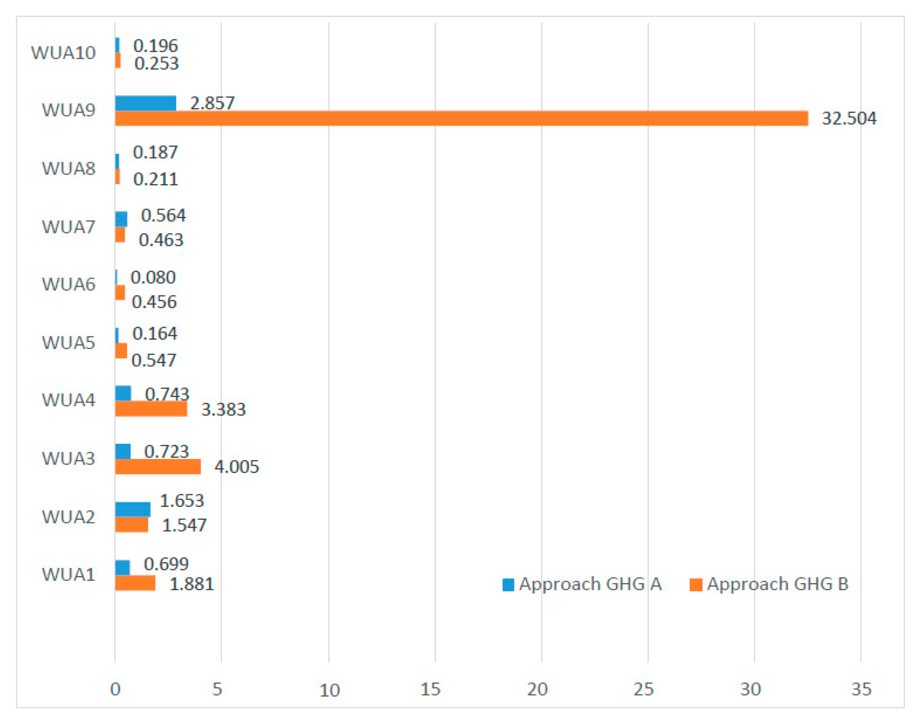
The comparison of emissions according to Approaches A and B (

Table 4. Comparative GHGs emissions/methodologies and GHGs cost (€/tCO₂e).

WUAs	Approach A (kgCO2e)	Approach B (kgCO2e)	GHG Cost (Approach A)	GHG Cost (Approach B)
WUA 1	698,932	1,881,096	3,921,049	10,592,784
WUA 2	1,652,652	1,547,013	9,662,283	8,722,866
	1,257,952	677,196	7,337,905	3,815,716
	22,691	126,462	134,035	714,792
	372,009	743,355	2,190,343	4,192,358
WUA 3	723,379	4,004,835	4,204,389	22,514,099
	226,668	1,654,215	1,337,465	9,298,159
	496,711	2,350,621	2,866,924	13,215,940
WUA 4	743,476	3,382,884	4,513,451	19,079,867
WUA 5	164,262	547,264	929,467	3,080,739
WUA 6	79,819	456,440	502,127	2,967,688
WUA 7	564,156	462,787	3,762,490	2,883,768
WUA 8	186,644	211,012	1,075,423	1,188,009
	13,469	147,267	78,765	826,100
	133,728	30,981	770,558	176,937
	6864	7556	39,376	43,341
	32,583	25,208	186,724	141,631
WUA 9	2,586,911	32,503,714	14,648,714	185,911,984
	64,176	1,019,386	348.903	5,718,755
	738,150	11,210,263	4,264,986	64,010,602
	570,260	6,524,128	3,286,365	36,730,841
	342,513	4,104,375	1,922,024	24,010,594
	573,817	5,900,837	3,169,931	33,044,687
	297,995	3,744,725	1,656,505	22,396,505
WUA 10	196,366	252,597	1,028,890	1,281,326
	67,844	136,283	344,523	690,271
	83,200	85,440	437,816	433,906
	45,322	30,874	246,551	157,149

Source: Own elaboration.

and Figure 3) shows the kgCO₂e values emitted by the studied WUAs. Although Approach B results the GHG emissions, it is observed how these values are globally double the emitted by the pumping stations. However, if an individual analysis of each WUA is considered, it is found that only WUAs 2, 8 and 10 present similar values (Figure 3). This can be interpreted as the WUAs are being endowed and irrigated according to the water needs for each crop. In the other WUAs, water deficit is very important since the amount they receive is a third of their water needs. The values of the deficit are highest in WUAs 3, 5 and especially 9.

WUAs are emitting less GHG than they could if they were well equipped. The scarcity of water in this area results in less GHG emissions.

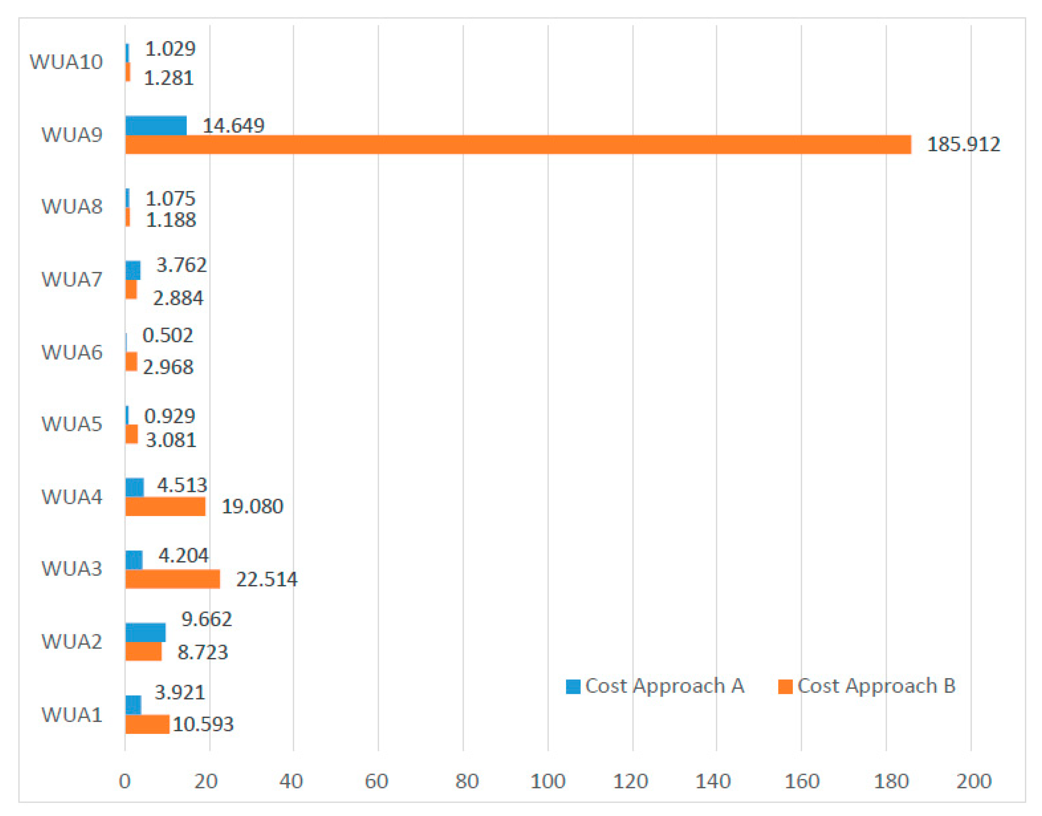
Finally, according to both methodologies, the economic impact of the emissions generated by the management of irrigation water in the studied WUAs is quantified (Figure 4). In 2017, in accordance with from the website of the European CO₂ Trading System [5], the average value is €5.83/tCO₂e. This average value, which is provided monthly, shows that in that year it was higher in the months of October to December, exceeding €7.3/tCO₂e, and lower in April and May with a value of €4.7/tCO₂e.

The information shown in Table 4 and Figure 3 and Figure 4 was timed based on the energy consumption according to the monthly operation of each equipment.

A breakdown report of the total GHG emissions based in both methods was developed for all WUAs (Table 3 and Table 4). Estimating the carbon footprint in CO₂e and CHG emissions of any activity is a difficult and complex task. It is a great step that several authors have decided to make a first approach to the calculation of GHG emissions related to the management of water in irrigation, since it is an aspect that has hardly been addressed. Although it is necessary to continue advancing to perfect the methodology carried out, the great effort made is evident.

As these are an application of recent methodologies, there are still aspects that must continue to be improved to achieve greater consistency and precision. In this sense, the lack of information has been detected in some analyzed studies, such as the origin of the water used in irrigation, the type of pumps used and their energy efficiency or the irrigation system installed and its application efficiency. In some studies, given the impossibility of measuring factors, estimates were applied, which, being a pragmatic solution, the choice of these variables has not always been justified in detail. The object of each study is specific, and the precision and detail of the indices used varies depending on the objective to be met.

In this paper, two methodologies for estimating GHG emissions are presented, and the results, units used and conclusions obtained are heterogeneous. In some studies, the results of GHG emissions related to the volume of water applied have been exposed, while, in other studies, they have been related to the yields of the crops, the use of energy, the area of cultivation and even in a general way without associating them to any other factor. In addition, different units have been used when expressing the volume of water applied, the energy demanded or the GHG emissions, another factor that shows the lack of consensus when expressing the results. Therefore, comparing the results of the studies is a confusing task that requires a previous step to adapt these units to the same expression.

In some studies, the energy demanded by the irrigation system has been included with the other electrical inputs (lighting, ventilation, heating, etc.). There should be a consensus to determine GHG emissions and establish a clear division of each component or aspect, since this way the associated CO₂-eq emissions with each part of the water management system could be more precisely determined.

In general, a reduction in the water footprint associated with irrigation leads to a reduction in the carbon footprint associated with this activity. This synergy achieves the maximum results when the irrigation water comes from underground, since the less water to be extracted, the less GHG emissions are generated, as the extraction of groundwater is the activity with the highest demand for conventional electrical energy in the irrigation. The improvement and modernization of the equipment that intervenes in the management of water in irrigation entails a reduction in the CO₂-eq emissions since energy and water application efficiency increases considerably.

To carry out strategies to reduce the water and carbon footprint associated with the management of water for irrigation, an economic injection is needed in agricultural holdings, from both single owners and communities of irrigators of several users. Public administrations are playing an important role when offering financing facilities or technical advice, since, in many cases, due to both ignorance and lack of financial means, no changes are made for this purpose.

In the case of electrical energy, the transformation index is varied due to the generation mix used in each study area. This has been a key factor in calculating GHG emissions from irrigation water management, so it is important to delve into this aspect, analyzing and taking into account the variations that occur in the transformation rate of the electrical energy, and thus calculating the GHG emissions generated in a more precise way. Although the carbon footprint has a global effect, its calculation procedure must consider local aspects that, nowadays, are easier to obtain by increasing the possibility of monitoring irrigation systems.

The incorporation of the irrigation activity in life cycle analysis, which will be a fundamental requirement in the near future, demands systems for monitoring, accounting and validating the energy consumption in quasi-real time that allow determining the CO₂-eq and CHG emissions associated with this exercise.

4. Conclusions

The theoretical calculation of the minimum and maximum potential GHG emissions is very useful as a tool for quantifying the possible extremes of the minimum and maximum CO₂-eq and CHG emissions generated in the management of irrigation water. Although the positioning of the GHG emissions calculated between the maximum and minimum potential depends on the transformation index and when the consumption occurs, affecting the dispersion of data, the necessary knowledge is generated to establish the minimum and maximum thresholds of these GHG emissions and thus having a reference on which to compare the current management mode.

The studied Southeast Spanish WUAs are under-endowed in terms of water resources. The demand for irrigation water is much higher than what they actually are receiving.

In the agricultural sector, WUAs play an important role in energy savings. Most of the energy consumption of this sector is managed by these organizations, which also manage water resources for irrigation during the year. Therefore, a suitable water and energy control is necessary, and the investment in CO₂ emissions is considered a low-cost one against the obtained environmental benefits. The applied methodology compares the irrigation systems of several WUAs, allowing the critical points of the irrigation systems of the WUAs to be analyzed. This methodology was validated in a different location than the previous case studies in the literature.

According to the analysis of the studies that are part of this work, a series of measures are proposed to to reduce the GHG emissions related to the management of water in irrigation. In areas where groundwater for irrigation is representative, controlling piezometric levels, as well as their evolution throughout an irrigation campaign, is decisive to accurately estimate the CO₂-eq and CHG emissions associated with this activity, which is the first step to reduce it. Old facilities should be replaced with low water and energy application efficiency with modern facilities. For this type of improvement to spread throughout the territory, financial support from public administrations in the form of incentives or financing, as well as in the form of technical advice, is essential. Pressurized irrigation systems should be used when the applied water is of underground origin, since most of the energy demand is needed in the extraction process. By pressurizing irrigation systems, it is possible to reduce losses in transport and a more efficient application in the field, which reduces the volume of water extracted. The knowledge of the optimal time and volume of irrigation water, avoiding water percolation. In addition, a controlled deficit irrigation should be carried out, so that the productions are the largest possible with the least amount of water applied. Technical support is essential to carry out controlled deficit irrigation.

Having a more precise knowledge of the emission factor of electrical energy at all times is necessary in this kind of studies. This is related to the suitable determination of the period in which the emission factor is low, in order to schedule irrigation based on this information. It is a measure that concerns other factors, such as the price of energy in each tariff period, breakdowns, etc., in addition to the involvement of public administrations. The great variability in the methodologies used leads to obtaining different results. Using different energy transformation indices, without stopping to justify the choice in each case or establishing different scopes of GHG emissions to be included in the studies, makes it difficult to compare the results obtained. Therefore, it is necessary to unify the methodology, establishing a procedure that covers different situations and making it as universal and precise as possible.