Evaluation of the Impact of Climate Change on Runoff Generation in an Andean Glacier Watershed
by
 , and
, and
Rossana Escanilla-Minchel
1,* ,
,
Hernán Alcayaga
1,
Marco Soto-Alvarez
1,
Christophe Kinnard
2 and
Roberto Urrutia
3 1
Escuela de Ingeniería en Obras Civiles, Universidad Diego Portales, Santiago 8370109, Chile
2
Department of Environmental Sciences, University of Québec at Trois-Rivières, Trois-Rivières, QC G8Z 4M3, Canada
3
Facultad de Ciencias Ambientales/Centro EULA-Chile de la Universidad de Concepción, Concepción 409541, Chile
*
Author to whom correspondence should be addressed.
Water 2020, 12(12), 3547; https://doi.org/10.3390/w12123547
Submission received: 18 August 2020
/
Revised: 27 October 2020
/
Accepted: 15 December 2020
/
Published: 17 December 2020
(This article belongs to the Special Issue Whither Cold Regions Hydrology under Changing Climate Conditions)
Abstract
:Excluding Antarctica and Greenland, 3.8% of the world’s glacier area is concentrated in Chile. The country has been strongly affected by the mega drought, which affects the south-central area and has produced an increase in dependence on water resources from snow and glacier melting in dry periods. Recent climate change has led to an elevation of the zero-degree isotherm, a decrease in solid-state precipitation amounts and an accelerated loss of glacier and snow storage in the Chilean Andes. This situation calls for a better understanding of future water discharge in Andean headwater catchments in order to improve water resources management in glacier-fed populated areas. The present study uses hydrological modeling to characterize the hydrological processes occurring in a glacio-nival watershed of the central Andes and to examine the impact of different climate change scenarios on discharge. The study site is the upper sub-watershed of the Tinguiririca River (area: 141 km2), of which nearly 20% is covered by Universidad Glacier. The semi-distributed Snowmelt Runoff Model + Glacier (SRM+G) was forced with local meteorological data to simulate catchment runoff. The model was calibrated on even years and validated on odd years during the 2008–2014 period and found to correctly reproduce daily runoff. The model was then forced with downscaled ensemble projected precipitation and temperature series under the RCP 4.5 and RCP 8.5 scenarios, and the glacier adjusted using a volume-area scaling relationship. The results obtained for 2050 indicate a decrease in mean annual discharge (MAD) of 18.1% for the lowest emission scenario and 43.3% for the most pessimistic emission scenario, while for 2100 the MAD decreases by 31.4 and 54.2%, respectively, for each emission scenario. Results show that decreasing precipitation lead to reduced rainfall and snowmelt contributions to discharge. Glacier melt thus partly buffers the drying climate trend, but our results show that the peak water occurs near 2040, after which glacier depletion leads to reducing discharge, threatening the long-term water resource availability in this region.
1. Introduction
Water from glacier melt plays a vital role as a water resource for population located downstream in high mountain watersheds [1]. This natural water storage is being affected by climate change, as the reduced volume of glacier causes net losses in water storage, leading to significant but ephemeral increases in runoff during the ablation period [2]. Worldwide glacier retreat is threatening the sustainability of water resources in mountain regions, demonstrating the need to quantify the effects of climate change in these areas [3].
The central Andes are the main source of freshwater in Chile. The Andean cryosphere acts as a natural reservoir, storing large volumes of water in solid state. As such, high mountain watersheds exert a significant control on the production of runoff during the summer ablation period [4,5,6]. This, along with the constant population increase and urban expansion towards higher elevations areas, has led to an increase in water consumption [7]. Therefore, pressure on water resources from different users and consumption sector (sanitary, agricultural, mining, hydroelectrical, tourism, etc.), along with climatic disturbances, has significantly increased the uncertainty regarding the availability of future water and its management [8].
Climate change has become one of the greatest challenges facing society [9], especially due to the uncertainty caused by impacts on water resources. Worldwide projections indicate an increase in average temperature, while average precipitations are projected to decrease in the dry regions of mid, subtropical latitudes [10]. These climate projections should lead to an increase in the elevation of the zero-degree isotherm, which will cause a decrease in solid precipitation [11], generating significant glacier retreat accompanied by calving and melting of important glacier masses. Therefore, watersheds with significant glacier and snow cover will be highly exposed to variations caused by climate change [12]. From a hydrological perspective, warming temperatures in nivo-glacial watersheds can cause a decrease in solid-state precipitation, which reduces snow accumulation and translates into variations of maximum discharges and changes in overall water balance [13]. In the context of the central Andes, a general drying trend has been observed over the last century especially over the last decade [14], along with warming temperatures [15] and rising snowlines [16]. Glaciers in the northern and central Andes have been retreating over the 20th century [17,18,19], and shifted from a slightly positive (2000–2009) to a strongly negative mass balance in 2009–2018 [20], in line with the mega drought occurring in Chile since 2010 [14]. However, the response of river discharge to ongoing and future climate and cryosphere changes can be highly catchment specific and requires detailed modeling at the catchment scale [21].
A central concept on the consequences of climate change on runoff from glacierized basins is that of the peak water: warming will typically cause a transient increase in runoff from increased glacial melt, until a point where the depletion of glacier mass causes the runoff to decrease [3]. The timing of the peak water depends on the climate trajectory, so that it is essential to determine the peak water timing for different emission scenarios in order to establish mitigation measures against the long-term decrease in glacial runoff and its consequences on ecosystems and access to fresh water [22].
In this context, analyzing the consequences of climate change becomes crucial in areas where a glacial and snow regime predominates [23]. Hydrological models are a key tool for this task, as they are capable of simulating the response of hydrological processes to climate, allowing possible changes in runoff generation to be projected and assessed [24]. There is a wide range of modelling strategies and approaches, the most common model classification being based on the level of spatial simplification (spatially distributed, semi-distributed and lumped) and model complexity (physically based and conceptual), among others [24]. The level of spatial simplification depends on the amount of data available in the study, while model complexity reflects the detail of process representation within the model. Complex models require more input data and require specifying many unknown parameters, leading to equifinality uncertainties that add up to structural uncertainties and climate scenarios uncertainties [25,26,27].
The main objective of this study was to evaluate the impact of climate change on surface runoff generation in an Andean glacial watershed. To this end, the semi-distributed Snowmelt Runoff Model [28] was coupled with the Glacier module proposed by Ismail and Bogacki [29], calibrated and validated against runoff observations. Subsequently, outputs from seventy ensemble GCM climate scenarios under two emission scenarios, RCP 4.5 and RCP 8.5, were used to generate the precipitation and temperature time series through statistical downscaling. These time series where used to force the hydrological model, generating an ensemble of seventy discharge projections, providing a range of variations from present to the end of the century and allowing to estimate the impact of future climate conditions on the hydrological regime of the watershed.
2. Study Area
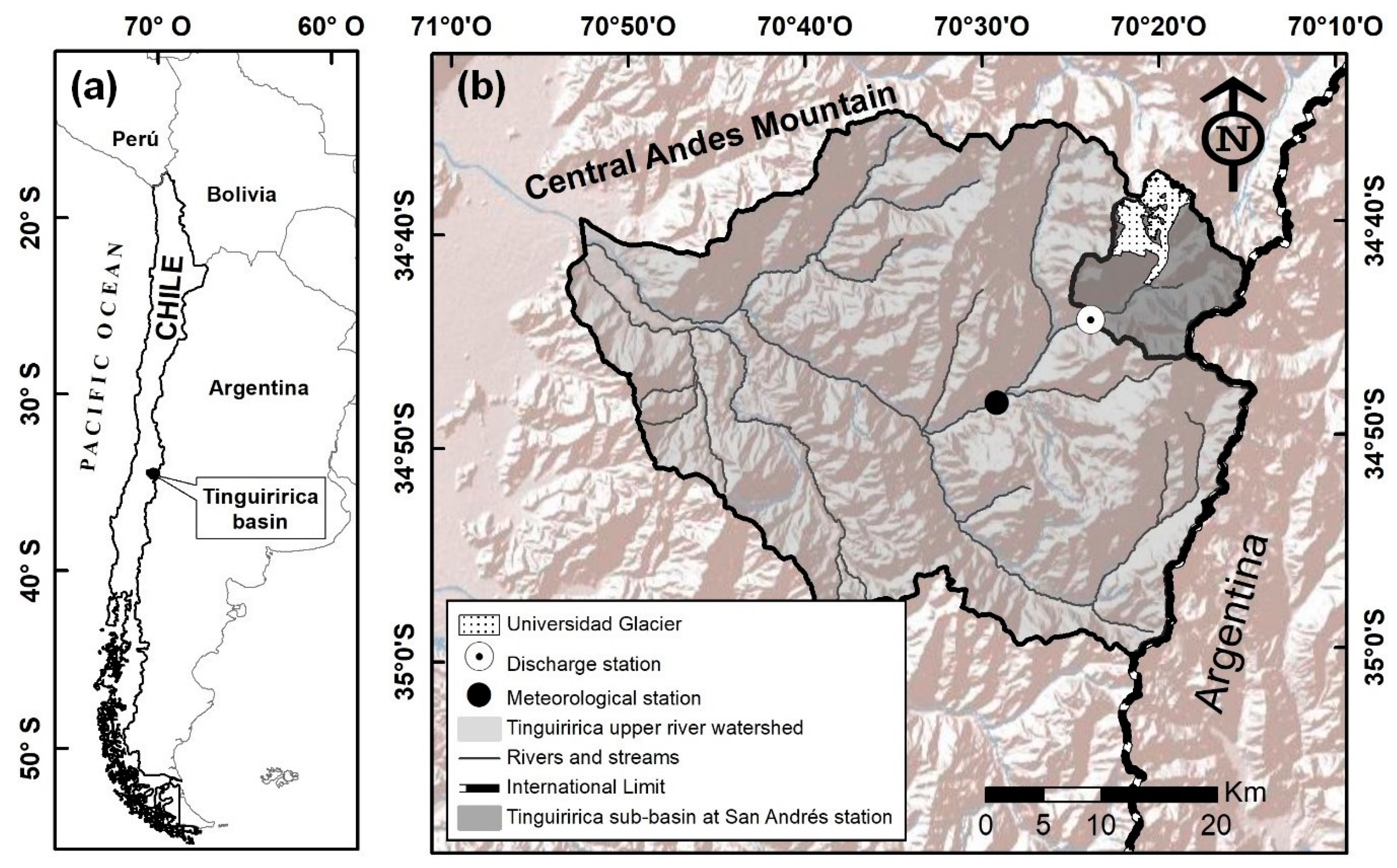
The study area is located in the central Chilean Andes in the O’Higgins Region (Figure 1a). It is a headwater sub-watershed of the Tinguiririca River watershed, which contains Universidad Glacier, the largest glacier in Chile outside Patagonia [30]. The Tinguiririca River (14,177 km2) is characterized by a mixed rain-snow hydrological regime, with two maximum discharge peaks each year. The first maximum occurs during winter (April to October) in response to increased rainfall at lower elevations, while the second peak occurs during the ablation period (November to March) in response to the melting of snow and glacier ice. The Universidad Glacier contributes between 20 and 25% of the total river runoff, based on available runoff observations [31].
The sub-watershed was delimited based on the location of the San Andrés discharge monitoring station, which belongs to the hydroelectric plant of the same name, approximately 1500 m downstream of the glacier front at an altitude of 1724 m.a.s.l. (Figure 1b). This sub-watershed has an area of 140.73 km2, 19.6% of which is glacier cover.
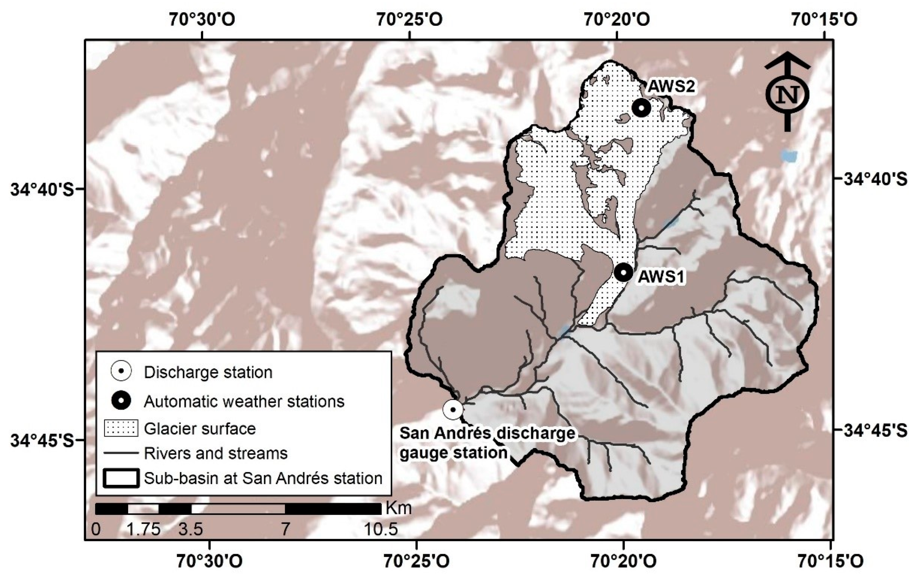
The Universidad Glacier is classified as a valley glacier and has a total area of 27.44 km2, with an altitude range of 2427 to 4944 m.a.s.l. It has two main accumulation zones (Figure 2), which join in the ablation zone, located below 2790 m.a.s.l. Due to the enormous precipitation deficit resulting from dry summers and the ongoing drought in Central Chile [14], the runoff contribution of the glacier is vital for the region [32], whose consumptive water use is mainly for agricultural irrigation.
In 2012, the Environmental Science Center EULA-Chile installed two automatic weather stations on Universidad Glacier (Figure 2) [30]. The first station (AWS1) is located in the ablation zone at 2790 m.a.s.l., while the second (AWS2) is located in the accumulation zone at 3629 m.a.s.l. [33]. These stations collected hourly data from November 2012 to November 2014. The closest permanent weather station is the Río Tinguiririca aguas abajo junta Río Azufre, hereafter denoted ‘Río Tinguirirca station’, located 18 km downstream of the San Andrés g auging station (Figure 1b) and in operation since 1980. EULA-Chile also collected glaciological information on Universidad Glacier. Mass balance was calculated for 2012–2014 using the glaciological method at a network of stakes and snow pits along the glacier centerline of the two glacier subbasins, and displacement was monitored at the stakes [30]. Mass-balance observations were used as a reference to project the future area of the glacier through a volume–area relationship.
3. Methods
3.1. Hydrological Model
3.1.1. Model Structure
The Snowmelt Runoff Model + Glacier is a semi-distributed hydrological model for simulating runoff on a daily scale in watersheds where snow and glacier melt dominate the runoff generation process. It has been successfully applied in over 100 snow-affected watersheds around the world, with areas up to 900,000 km2 and elevations up to 8840 m.a.s.l. [28]. The standard version has two runoff components, i.e., snow and rain; therefore, for this study a third module was used to add the glacier component [29]. The model has been used in other studies to simulate the hydrological response of watersheds in Chile. The effectiveness of the model has been notably verified in the Tinguiririca River at Bajo Briones, downstream of the studied sub-watershed, where a correlation coefficient of 0.88 was found between observed and simulated streamflow [34].
The model estimates the total quantity of water produced by glacier melt and snow, along with liquid precipitation in the watershed, with a daily time step through Equation (1):
where Q is the average daily discharge (m3 s−1); M, R and G are average daily snowmelt, liquid precipitation, and glacier melt (cm day−1), respectively; k is the recession coefficient (dimensionless); n is the index of the current day; i and m are the indices and total number of elevation bands. The expression represents a conversion factor to obtain the daily discharge units (m3 s−1).
Daily runoff due to snowmelt (M), glacier melt (G) and precipitation (R) in cm day−1 is calculated using Equations (2)–(4):
where S, G and R indices refer to the snow, glacier and rain components of runoff; A represents the areas dominated by the different components in km2; c is the runoff coefficient in these areas; ddf represents the degree-day factor for snow and aG for glacier ice (cm °C−1 day−1); T is the number of positive degree days of air temperature (°C day) and P is liquid precipitation (cm). The SRM+G calculates snow and glacier melt based on positive temperatures; therefore, no glacier or snowmelt occurs when air temperatures are negative.
In this study, discharge observations available at the San Andrés station for the hydrological years from April 2008 to March 2014 were used for model calibration and validation, using the even years for calibration and odd years for validation, to reduce climatic dependence in the calibration [35]. The data from the on-glacier automatic weather stations, available from November 2012 to November 2014, were used to determine the precipitation and temperature gradients on the watershed. Daily precipitation and temperatures from the permanent Río Tinguirirca weather station were used to force the model.
3.1.2. Model Parameters
In watersheds such as the one studied here, the runoff modelled by SRM+G depends on air temperature, the degree-day factors for snow and glacier melt, and the snow and glacier areas in the watershed [29]. The degree-factor for snowmelt is calculated following the relationship established by Rango and Martinec (1996) [36], as shown in Equation (5):
where is the snow density and is water density, both in kg m−3. The degree-day factors for snow varies during the ablation months (November to March), with a maximum value of 0.55 cm °C−1 day−1 derived from Equation (5) in March, with a snow density of 500 kg m−3, and a minimum value of 0.10 cm °C−1 day−1 in November. The minimum value and the intermediate values (for December to February) are calibrated through density in order to better adjust the representation of the model during the thaw period. The seasonality in the snow ddf accounts for the unaccounted seasonal variation in incoming solar radiation and snow aging, the latter of which leads to increasing snow density, decreasing albedo and increased ablation [37,38,39,40]. The value of ddf is set to zero on the coldest winter months (April to October) to account for reduced incoming solar radiation and limited or no melting in winter. Unlike snow, glacial ice does not have significant albedo variations during the year [40]. Furthermore, this particular glacier has few debris on its surface, which are only located in the lower ablation zone); therefore, a constant degree-day factor for glacier melt () was used based on the study by Bravo et al. (2017) [31] at Universidad Glacier, who used a value of 0.8 cm °C−1 day−1 based on values for glacier ice from Hock (2005) [37]. Constant values have also been used in the Himalayas [29,41] and in other basins of central and southern Andes [42,43,44].
Constant runoff coefficients were used for snow, glacier, and rain areas. The values used in this work for the snow and ice runoff coefficients were taken from Ismail and Bogacki (2018) [29], for glacial watersheds in India, where cS = 0.8 and cG = 0.7. The runoff coefficient for rain area was adjusted as part of the model calibration. The recession coefficient k was calculated according to Rango and Martinec (1996) [36] using Equation (6):
where k is the recession coefficient; x and y are constants that must be determined for the analyzed watershed and Q is the observed discharge. The recession coefficient varies on a daily time step, while the values of x and y are established as constants. Here, one pair of values (x, y) was used for the ablation period (November to March) and another for the precipitation period (April to October). The x and y values were set as model calibration parameters and determined through an optimization method using genetic algorithms. The automatic calibration method using genetic algorithms [45] seeks values for the calibration parameter that optimize the statistical indicators of model fit, which are presented in Section 3.2.
Air temperature was distributed to the catchment using a mean altitudinal temperature gradient of −6.8 °C km−1 calculated from the two weather stations located on the glacier (Figure 2). Precipitation were distributed over the catchment on each elevation band with a precipitation gradient, expressed by Equation (7):
where PPi represents a percentage of precipitation measured at the Río Tinguiririca meteorological station in elevation band i; Zi is the mean height in meters above sea level of the band i. This precipitation gradient was obtained through the relationship between the rainfall measured in AWS1 in summer months (Figure 2) (at 2790 m.a.s.l.) and the Río Tinguiririca meteorological station (at 1134 m.a.s.l.) for a one-year period of analysis. The obtained parameter for this study are consistent with those calculated by Ragettli et al. (2014) in the central Andes [46]. Four elevation bands were used to distribute precipitation and to calculate snow and glacier melt over the catchment, based on the precipitation and temperature gradients. A threshold temperature of 0 °C was used to separate liquid and solid precipitation. The parameters used in the model are listed in Table 1.
Glacierized areas were obtained from the public glacier inventory available from the Dirección General de Aguas (hereafter denoted DGA) in 2014 [47]. According to DGA (2014), Universidad Glacier retreated by 0.03 km2 year−1 during de 1945–2011 period, reaching an area of 27.44 km2 in April 2013. The snow cover area was determined on a daily scale using the Moderate Resolution Imaging Spectroradiometer (MODIS) Snow Cover Daily L3 Global 500-m grid satellite product (MOD10A1) [48,49]. This product provides the normalized difference snow index (NDSI), calculated using Equation (8):
where MODISB4,B6 are bands 4 and 6 of the sensor. Grid cells with a NDSI index larger than 0.4 were classified as snow [50]. A filter was applied to discard the whole daily grid when cloud cover was greater than 20%, and the missing grid was interpolated using the previous and next day with available information through nearest neighbor interpolation. Finally, the area of liquid precipitation is determined with the temperature lapse rate; if precipitation occurs within an elevation band with temperature greater than zero, then the area of that band not covered by snow or ice is contributes liquid precipitation.
3.2. Model Effiency Indicators
For both the calibration and validation periods, four statistical fit indicators were used to measure the model efficiency, based on the comparison between the observed (O) and simulated discharges (P).
The coefficient of determination (r2) is defined as the squared Pearson’s correlation coefficient [51] and is calculated according to Equation (9):
where is the average of the observed values and is the average of the simulated values.
The Nash–Sutcliffe Efficiency (NSE), proposed by Nash and Sutcliffe (1970) is a normalized statistic that estimates the relative magnitude of the residual variance compared to the measured data variance [52]. A score of NSE = 1 indicates a perfect simulation, NSE = 0 indicates that the simulation is not better that using mean observations as sole predictor, and NSE < 0 indicates that the simulation is worse than using mean observations (Equation (10)):
The root mean square error (RMSE) is estimated through the square root of the difference between the observed and simulated values over the total number of data [52] and is calculated according to Equation (11):
where N is the total amount of data.
The modified Kling–Gupta Efficiency (KGE’) is an improvement on the Nash–Sutcliffe Efficiency proposed by Kling and Gupta (2009) [53], in which the correlation, deviation and variability components are weighted equally, solving systematic problems of maximum value underestimation [54]. The modified version [55] is calculated according to Equation (12):
where r is the Pearson’s correlation coefficient; α is the ratio of the coefficient of variation of the observed and simulated values; δ is the ratio between mean simulated and observed discharges.
The r2, NSE and KGE′ indicators have an optimum of 1, while RMSE has an optimum of 0.
3.3. Climate Change Scenarios
In accordance with the Fifth Assessment Report (AR5) [10], this study focused on two of the four climate change scenarios, better known as Representative Concentration Pathways, RCP 4.5 and RCP 8.5. The first represents a stable scenario where the emission of greenhouse gas increases until the mid-21st century [56,57], while the second is a more unfavorable and high-emission scenario where emissions keep increasing exponentially to the end of the 21st century [58].
Based on the selected emission pathways, ensemble simulations from 18 global circulation models (GCMs) were selected from the Coupled Model Inter-Comparison Project Phase 5 (CMIP5) [59], providing a total of 70 future climate simulations. The ensembles are a set of simulations that characterize climate projections, where the differences in the initial conditions and the formulation of the models give rise to different evolutions of the climate system that can contribute information on the uncertainty associated with the error of each model [10]. The GCMs used in this study for climate simulations are presented in Table 2.
Downscaling
The GCMs have a spatial resolution that varies between approximately 1.5° and 2.5°, which is inadequate for the spatial scale of this study because the representativeness of the involved climate phenomena is lost, preventing characterizations at the watershed level [60]. As a result of this issue, there has been increasing use of regional climate models (RCMs), which transform the spatial scale of GCMs to a finer scale that is more applicable to watershed-level studies, with study areas under 40,000 km2 [61]. The approaches used to downscale GCMs can be dynamic (use of regional climate models) or statistical. In both cases it is sought to eliminate the systematic bias in global models and transform the coarse GCM climate outputs towards at a reduced spatial resolution [62]. The dynamic methods have demanding computational requirements, such that the use of statistical methods is more common. In this study, the Quantile Mapping Bias Correction method was used to downscale the GCMs outputs to the watershed. This method uses as distinct bias correction for the percentiles of the cumulative distribution function (CDF) of the GCMs, with respect to the percentiles of the observed data. That is, for each GCM climate datum a CDF is determined, through which an occurrence probability is obtained. Subsequently, the GCM CDF is adjusted to the observed CDF, removing the bias and allowing it to be quantified in order to eliminate it in the projection phase [63]. The foregoing is defined according to Equation (13):
where Po is an observed climate variable; Pm is a variable simulated by the GMCs; Fm is the CDF of Pm and Fo−1 is the inverse CDF corresponding to Po.
In the case of precipitation, a two-parameter Gamma probability distribution was used, as expressed in Equations (14)–(16) [60], while for temperature a normal distribution was used, according to Equation (17) [64].
where X is the variable to evaluate, µ is the average of the total time series of data, and σ is the standard deviation of the series.
Three periods were defined for the downscaling process. The first period is associated with observed climate data (temperature and precipitation) from 1980 to 2005 and is referred to as the observed historical period. Historical climate data were obtained from the meteorological station Río Tinguirica. The second period covers the same period (1980–2005), but includes the climate data simulated by the GCMs, and is referred to as the simulated historical period. Lastly, the third period extends from 2006 to 2100 and corresponds to climate data projected by the GCMs and is referred to as the projected period.
3.4. Projections
Future discharge was projected by forcing the hydrological model with the downscaled GCM precipitation and temperature, extrapolating from the weather station to the rest of the basin, using the model parameters in Table 1. To estimate future glacier area, a volume-area scaling approach was used, following the empirical relation in Equation (18) [65]:
where V is the glacier volume in km3, S is the glacier area in km2, and γ and c are constants. In this case, γ was set to 1.357 following Bahr et al. (1997) [66], and k is derived from Universidad glacier’s initial volume V(t=2009) = 1.67 km w.e.3 and initial area S(t=2009) = 29.03 km2, which results in k = 0.017 km3−2γ. These initial volume comes from an interpolation of radio-echo soundings carried out on the glacier for that year [67]. Knowing these constants, it is possible to project the area of the glacier from the simulated volume changes, through Equation (19) [68]:
where is the volume change, bn is the simulated net glacier mass balance and S is the glacier area. Computed negative (positive) changes in area are removed (added) starting from the lowest elevation band in the model. To estimate the future snow cover area, multiple regression models that relate the snow cover area to temperature and precipitation were used [69], following Equation (20):
where AS is the snow cover area in km2; T is the daily temperature in ºC and PP is daily precipitation in mm. The values of Tfactor, PPfactor and CI were determined for this study from multiple regression, using the same methodology used by Khadha et al. (2014) [69] for a two-year period and used on a daily scale. The seasonal snow area relationships were determined with Equation (20), as shown in Table 3.
This relationship, for all the seasons results in a coefficient of determination of r2 = 0.89, where the observed snow areas are compared with those simulated using Equation (20) for the years with data availability. Finally, the distribution of the calculated snow area among the four elevation bands was carried out by filling from the highest band to the lowest.
4. Results
4.1. Hydrological Model
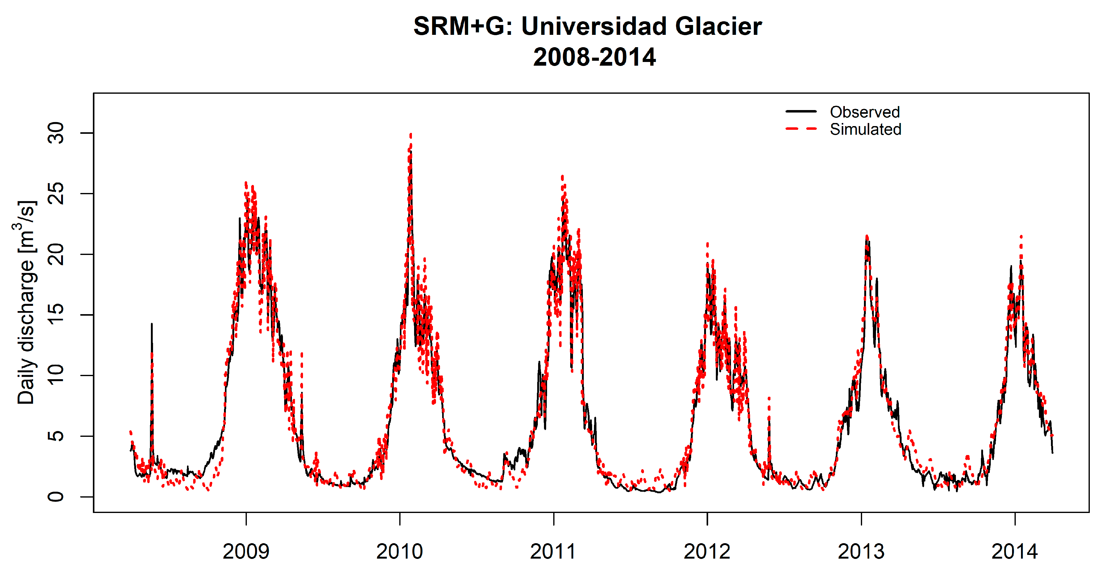
The hydrological model (SRM+G) results for the analyzed period (2008–2014) are presented in the hydrograph in Figure 3, while the correlations between observed and simulated discharges for the calibration and validation periods are shown in Figure 4a,b. Table 4 shows the model efficiency measures for the two subperiods. In the hydrograph in Figure 3, it can be observed that the SRM+G model better represents the observed discharge during the melting month (November–March), on runoff peaks. During the winter period, the model has more difficulties representing the observed low discharge.
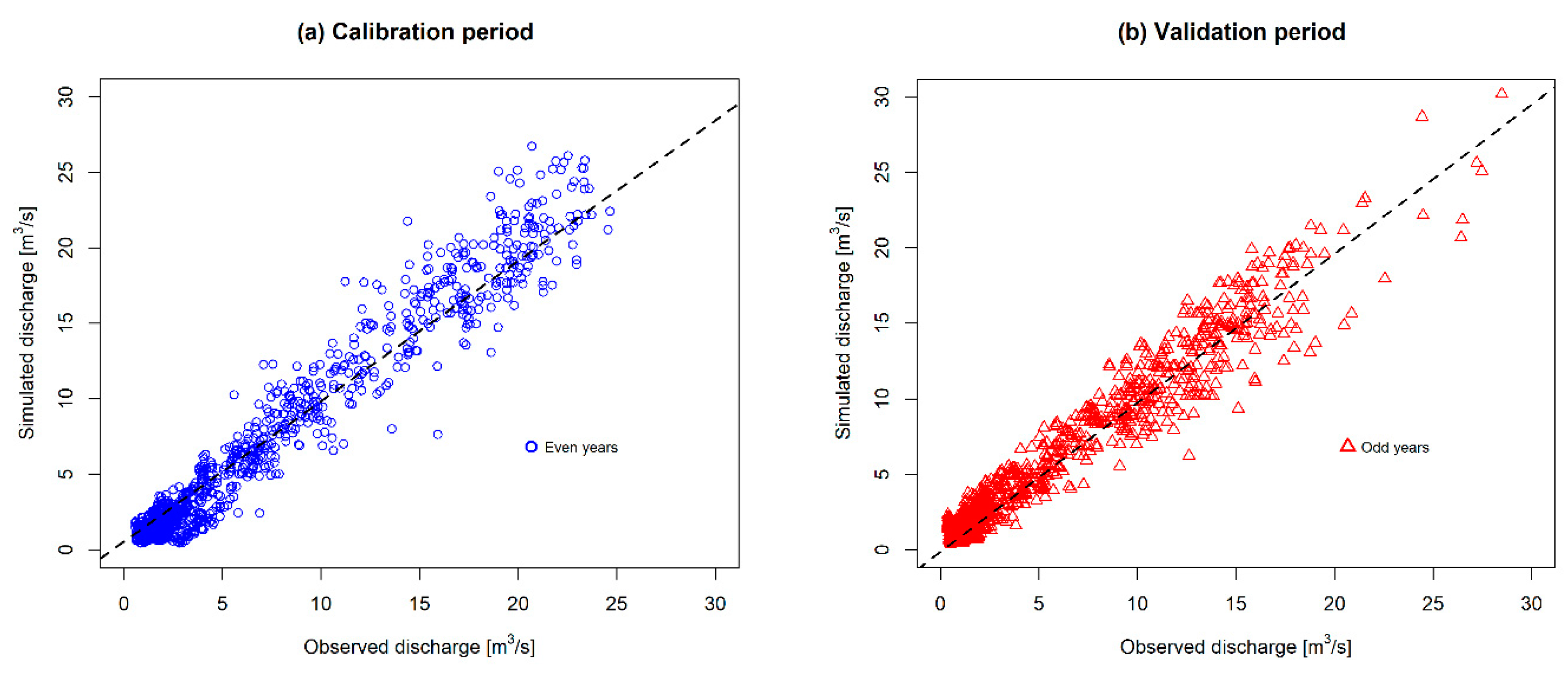
The scatterplots in Figure 4 show more dispersion for the validation periods than for the calibration period; however, both cases have a correlation trend consistent with the hydrograph in Figure 3, with more dispersion for discharges greater than 20 m3/s. The r2, NSE and KGE are above 0.70 and in some cases close to 1 (Table 4). Usually, a value of 0.7 or more for these indicators indicates efficient modeling [70].
4.2. Climate Change
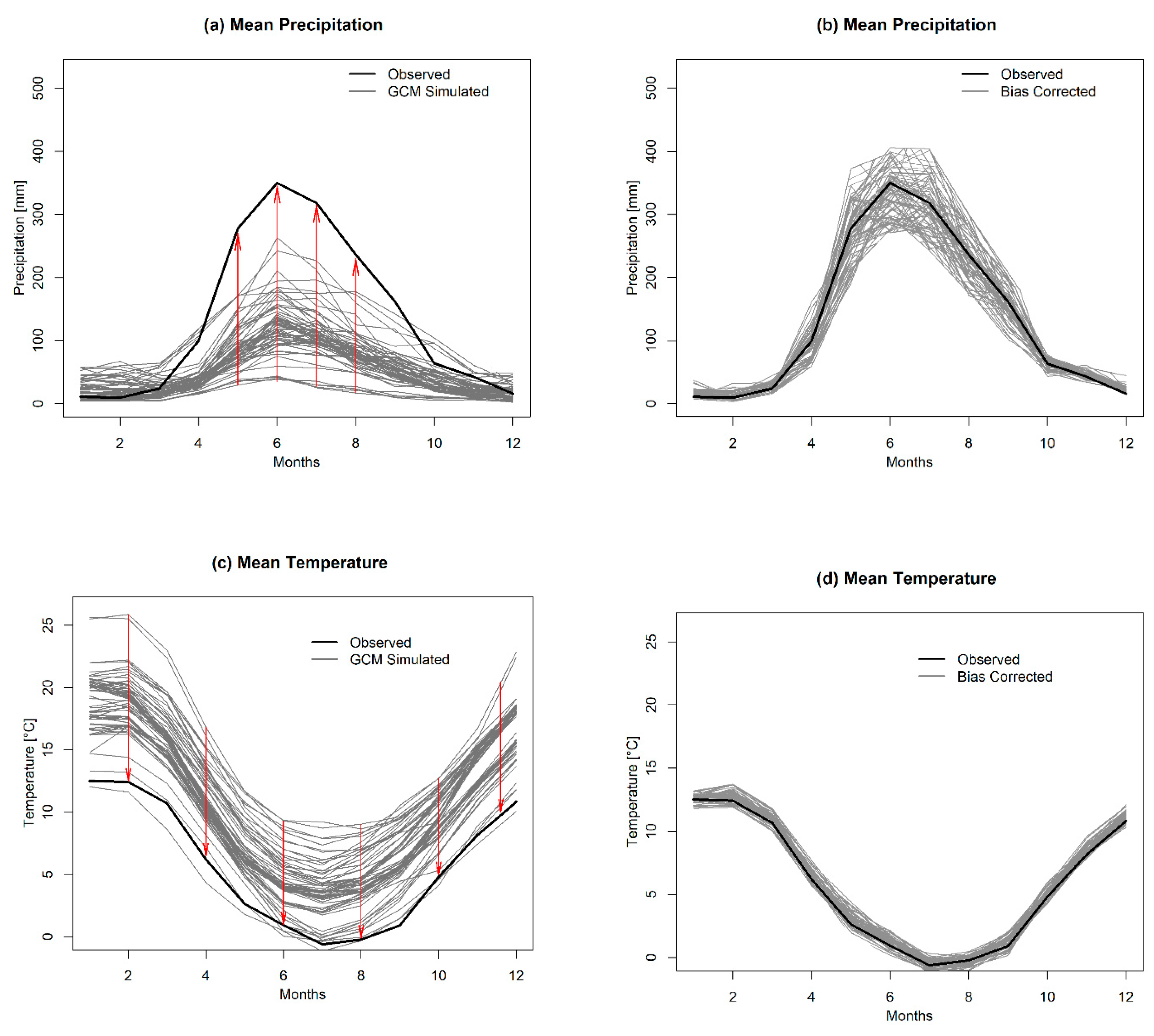
In Figure 5, the result of the statistical downscaling of the monthly averages of both precipitation (Figure 5a) and temperature (Figure 5c) are shown. The methodology was applied for both emission scenarios (RCP 4.5 and RCP 8.5) and the bias of the 70 GCMs used in this study was corrected (Figure 5b,d).
In Figure 5a, it can be observed that precipitation is overestimated in summer by some models, while it is underestimated by all models in the winter months. The red arrows indicate the expected effect of the bias correction procedure, i.e., bringing the models with greater dispersion closer to the expected mean. Figure 5b shows how the bias correction produces a better fit with the mean value of historical precipitation, although it generates a remaining dispersion around the observed values which is greatest in winter, reaching over 100 mm. In the case of temperature (Figure 5c) the same behavior is observed, with most of the models overestimating temperature, but in this case throughout the year. After the downscaling, little scatter remains and time series of temperatures correctly fit the observed historical period obtained (Figure 5d).
4.3. Projections
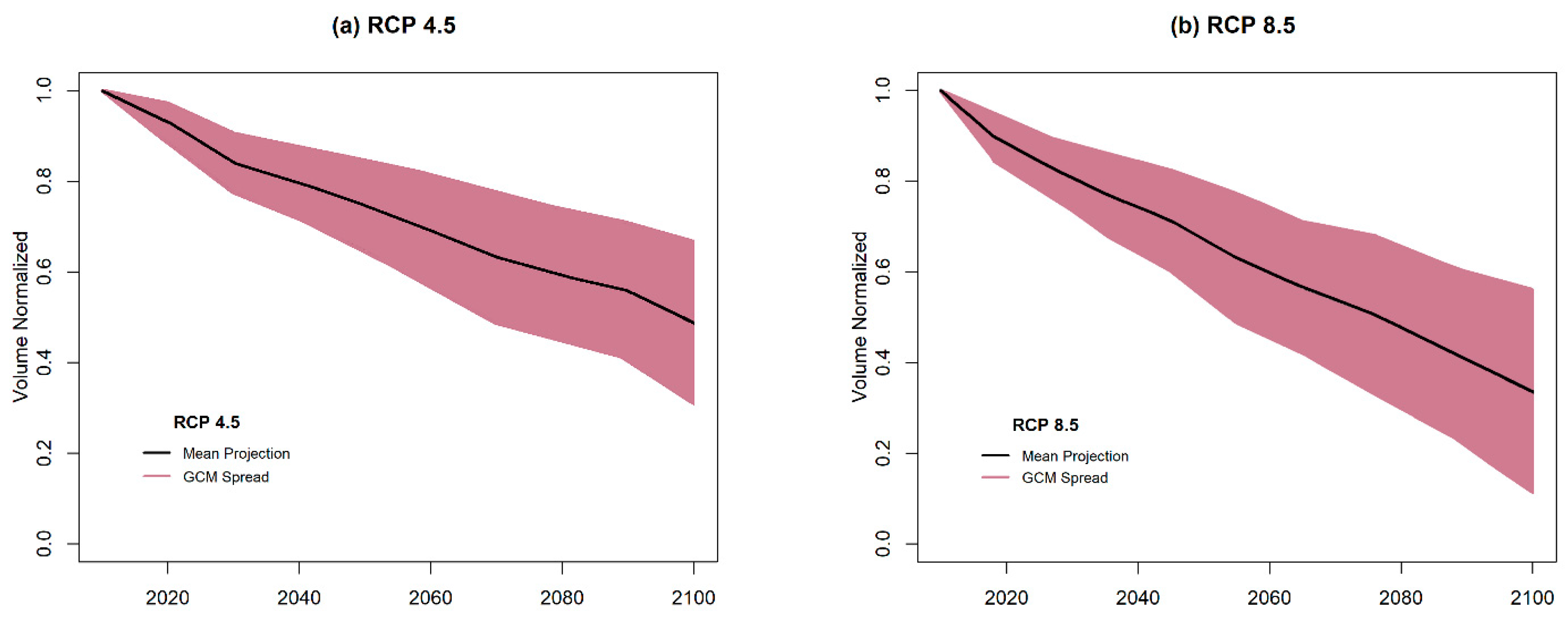
The simulated glacier mass balance for all GCMs analyzed shows a significant loss of glacier mass under both scenarios of climate change (Figure 6). Under the RCP 4.5 scenario, the ensemble of projected glacier volumes shows decreases ranging from 12 to 37% by 2050, while by the end of the century the ensemble volume loss trajectory reaches from 25 to 68%. The volume loss is greater under the RCP 8.5 scenario, decreasing between 20 and 48% by 2050 and reaching 51 to 84% by the end of the century.
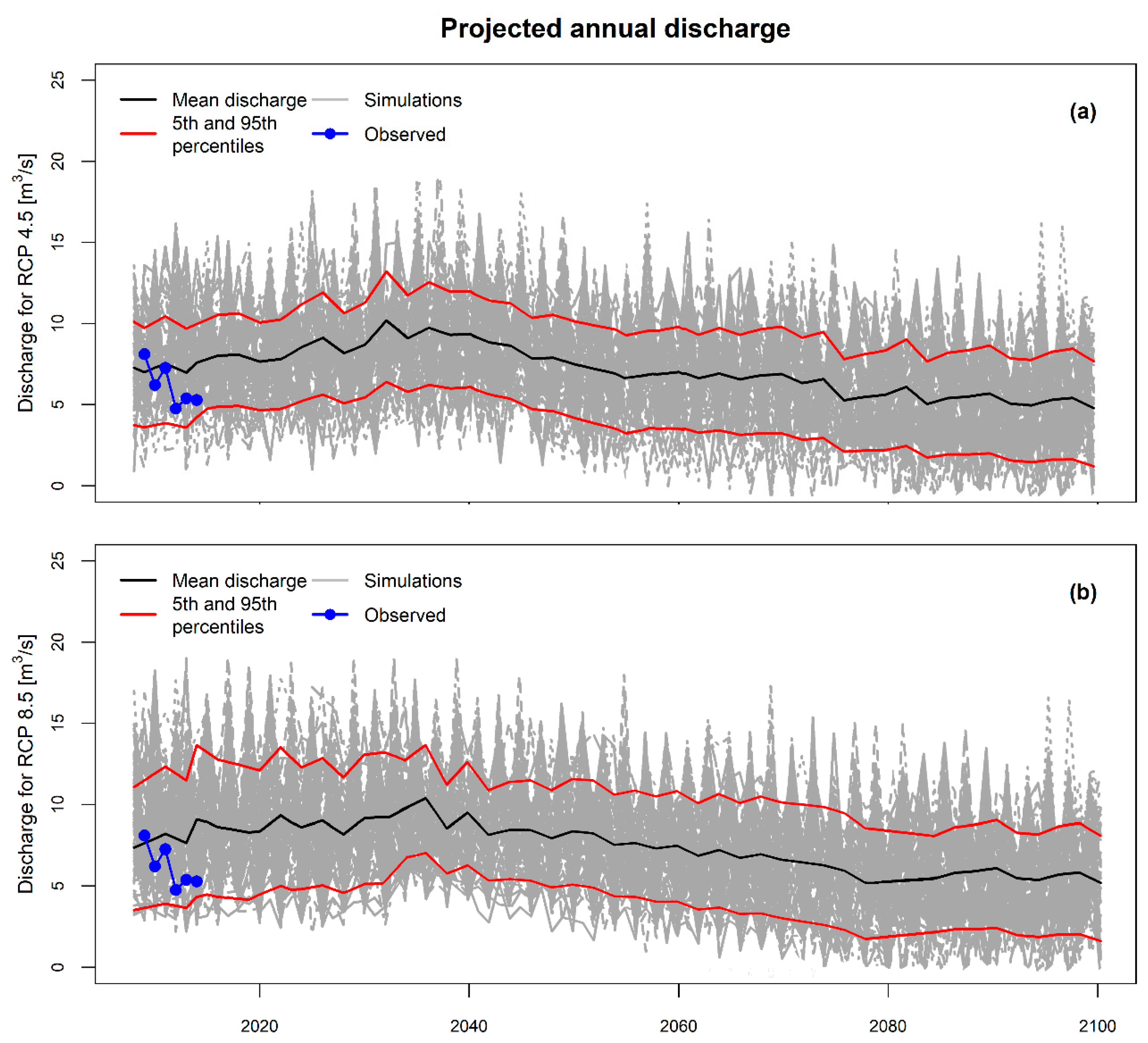
Table 5 shows the spread in downscaled GCM projections of climate variables for both emission scenarios in 2050 and 2100. There is a progressive decrease in precipitation and an increase in temperature for both scenarios, by 2050, with increasing differences between scenarios by the end of the century. The projected negative precipitation trend is particularly worrying in light of the mega drought that currently affects the area and which caused serious impacts on water resource availability. Based on the projections in Table 5, the simulated discharges using the downscaled precipitation and temperature under RCP 4.5 and RCP 8.5 scenarios are shown in Figure 7.
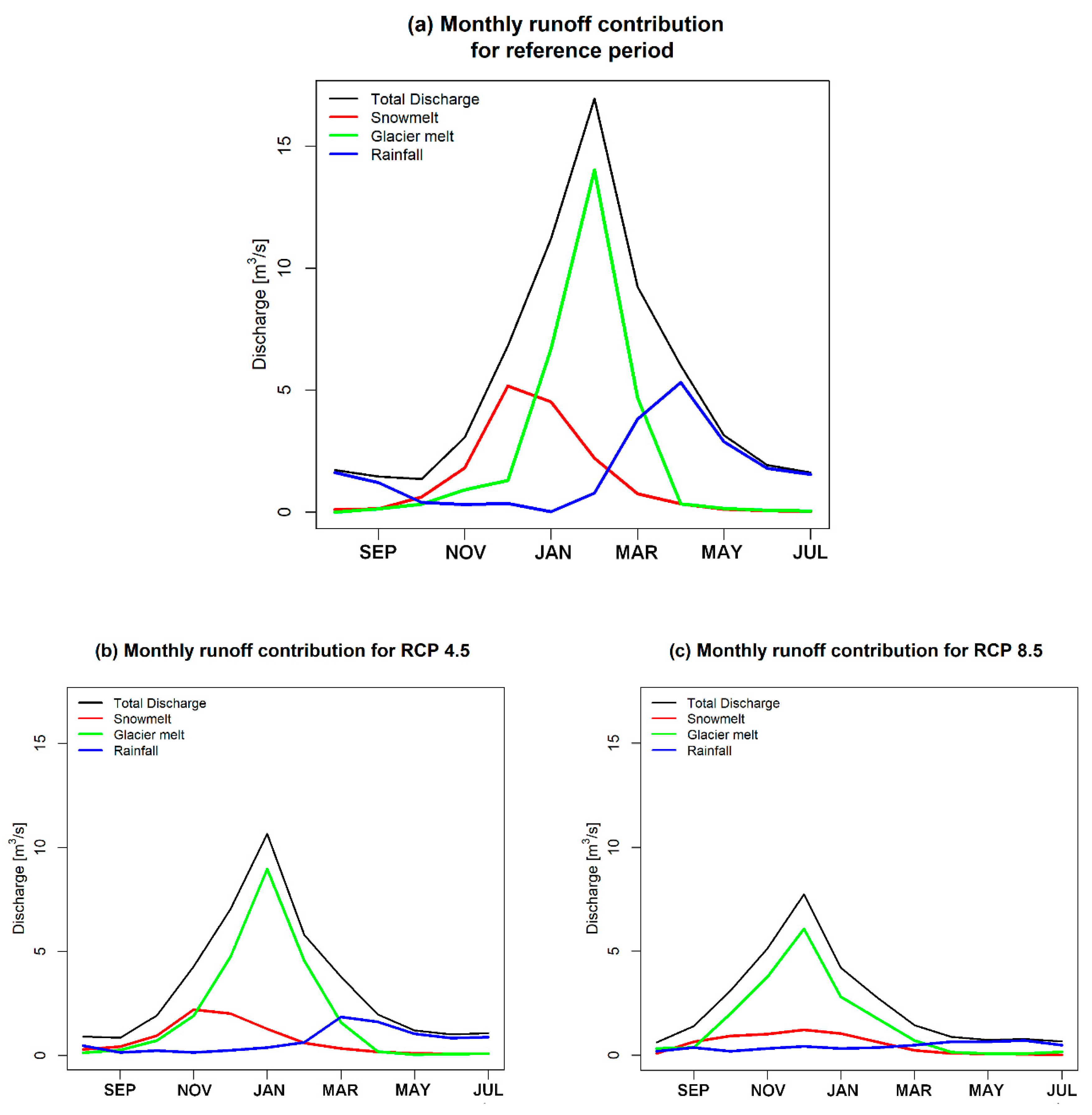
In both cases, there are 70 discharge series estimates, associated with each GCM and their ensemble members. An increase in runoff is observed for both scenarios, which reaches a peak around 2040, after which the runoff begins to decline. These results hence suggest that the peak water in this basin has not yet been reached and that increased glacier melting in response to warming will increase discharge until the peak water is reached around 2040. The decreasing discharge trend afterward is mainly due to decreasing glacier mass and the associated reduced contribution to runoff. A comparison of the two scenarios (RCP 4.5 and RCP 8.5) shows that in the first case, there is a sustained increase in mean annual discharge (MAD) over time until 2040, after which the MAD begins to decline. The peak water is better pronounced under scenario RCP4.5 and more subdued under RCP8.5. Increased mass loss under RCP8.5 depletes glacier volume faster (Figure 6), which restricts the contribution of glacial runoff by 2040 compared to RCP4.5. The changing runoff contributions are examined in Figure 8, where the contribution of the monthly average runoff for the year 2100 is shown under both emission scenarios RCP 4.5 and RCP 8.5.
The contribution of rainfall during the winter months (April–August) decreases by 2100 under both scenarios, due to the projected decreases in precipitation, as shown in Table 5. The reduced precipitation also explains part of the decreased snowmelt contributions in the future, which is further exacerbated by the conversion of snowfall to rain under warming temperatures. The decreasing snowmelt and rain contribution to streamflow are particularly worrying for the long-term sustainability of water resources downstream. Figure 8 shows that the bulk of discharge in this headwater catchments originates from glacier melt, and that the relative contribution of glacier melt to discharge increases in the future as runoff from snowmelt and rain decrease. As such, the flow remains dominated by glacial melt in the warmest months during the ablation period (October to March) under both scenarios but the peak contribution is much reduced an occurs earlier, by one month under RCP4.5 (in January) and by two months under RCP8.5 (in December). Hence, glacier melt constitutes a key buffer for the drying and warming trend projected in this region. However, and as seen in Figure 7, the peak water is reached around 2040 and the progressive depletion of glacier volume leads to decreasing glacier runoff onward, threatening the long-term sustainability of meltwater resources in this region.
5. Discussion and Conclusions
The Snowmelt Runoff Model + Glacier hydrological model was able to efficiently simulate the hydrological response of the studied watershed. Values above 0.8 were obtained for the four statistical indicators used to measure efficiency, indicating reliable simulations [70]. In comparison, the performance of the hydrological modeling of the Tinguiririca River at Bajo Briones for 1987–1988 by Escobar [34], which had a r2 of 0.88, was surpassed, even taking into account that the relative glacier cover is smaller within the contributing area of the Bajo Briones station. This increase in performance is attributed to the addition of the glacier module, which expectedly improves the hydrological response of the watershed. While the model has a greater percentage error during low-water periods, it correctly simulates melting periods when the water supply is greater. At an annual scale, the observed and simulated mean discharge values differ by only 7%. SRM+G is a hydrological model that can adequately represent runoff in basins with an area smaller than 500 km2. The model is thus particularly flexible for data-scarce regions where there is insufficient information to apply a fully-distributed model. The increased error observed in winter simulated discharge is due to the sensitivity of the model in distinguishing between liquid and solid precipitation. Another aspect that could improve the representation and efficiency of the model in the future would be to incorporate the effect of the debris on the lowermost glacier of the Universidad Glacier has, which could influence the spatial–temporal variation of the degree-day factor for ice and thus better represent the associated glacier ice melt processes [71,72,73]. It must be stressed that, for studies related to climate change, a greater number of years to calibrate and validate the selected hydrological model is recommended [74]. However, this is often difficult or impossible to achieve in high altitude, remote glacierized catchments such as the one studied here. Still, the good performance obtained in this limited data context suggests that the parsimonious modelling approach used is useful to project future discharge in response to climate change scenarios.
The bias correction procedure based on the quantile mapping method resulted in rescaled GCM precipitation that closely approach the observed values of the historical period, but with greatest remaining dispersion during winter, over 100 mm. This remaining scatter causes large positive discharge deviations that exceed the 95% confidence range (Figure 7). According to the downscaled projections, there will be a decrease in mean annual discharges with respect to current conditions. Mean annual discharge are projected to decrease by 18.1 and 43.3% by 2050 for RCP 4.5 and RCP 8.5, respectively, while by 2100, the projected decreases reach 31.4 and 54.2%. Similar responses have been projected in Chile, but with an even greater decrease, in the upper Juncal River basin [75], where mean annual discharge was projected to decrease by 62% for the RCP 8.5 scenario for 2100. Omani et al. (2016) show similar results [76] for a glacierized basin located in the central Andes, where they report a decrease in MAD of 17% for RCP 4.5 and 30% for RCP 8.5, by mid-century.
While according to the projections there will be an increase in water supply from the catchment until around 2040, it must be stressed that this increase will occur at the cost of a progressive and irreversible depletion in glacier volume, which will drive the reducing discharge trend from 2040 onward. The results of this work on glacier volume loss are consistent with other similar studies in Southern Andes, which reported losses around 25 and 68% for RCP 4.5 and 51 to 84% for RCP 8.5, both at the end of the century [3,77,78].
It has been shown that climate change has a negative impact in Andean zones because it increases the retreat of glacier masses and thus causes the irreversible loss of natural reservoirs, putting the sustainability of ecosystems into jeopardy and intensifying conflicts among stakeholders [23,79]. The projected ephemeral increase in meltwater outflux until 2040 simulated in this study thus represents a nonrenewable water source, as glacier depletion leads to reduced glacial runoff afterward. It has been estimated that the mega drought currently affecting central Chile will intensify by 2100 [80]. As such, the heavy dependence on water from the cryosphere may become a conflict scenario in various parts of the country near the end of this century. The temporary increase in water availability resulting from increased glacier melting could also have other consequences such as an increase in erosion and a reduction in infiltration time, which would affect aquifer recharge and the hydrological regime of downstream rivers [22]. Adaptation plans are highly recommended amid changes in the hydrological regime in these types of watersheds [81], especially those with intensive agricultural and industrial uses.
Author Contributions
Conceptualization, R.E.-M. and H.A.; Methodology, R.E.-M., H.A., C.K.; software, R.E.-M.; Formal Analysis, R.E.-M. and H.A.; Investigation, R.E.-M., H.A., M.S.-A., C.K.; Data Curation, R.E.-M. and R.U.; writing—original draft preparation, R.E.-M. and H.A.; writing—review and editing, H.A., R.U. and C.K.; visualization, R.E.-M., C.K.; supervision, H.A. All authors have read and agreed to the published version of the manuscript.
Funding
This research received no external funding.
Acknowledgments
This research was supported by project ANID/FONDAP/15130015, Water Research Center for Agriculture and Mining (CRHIAM).
Conflicts of Interest
The authors declare no conflict of interest.
References
- Migliavacca, F.; Confortola, G.; Soncini, A.; Senese, A.; Diolaiuti, G.A.; Smiraglia, C.; Barcaza, G.; Bocchiola, D. Hydrology and potential climate changes in the Rio Maipo (Chile). Geogr. Fis. E Din. Quat. 2015, 32, 155–168. [Google Scholar]
- Huh, K.; Baraër, M.; Mark, B.; Ahn, Y. Evaluating Glacier Volume Changes since the Little Ice Age Maximum and Consequences for Stream Flow by Integrating Models of Glacier Flow and Hydrology in the Cordillera Blanca, Peruvian Andes. Water 2018, 10, 1732. [Google Scholar] [CrossRef] [Green Version]
- Huss, M.; Hock, R. Global-scale hydrological response to future glacier mass loss. Nat. Clim. Chang. 2018, 8, 135–140. [Google Scholar] [CrossRef] [Green Version]
- Ayala, A.; Pellicciotti, F.; MacDonell, S.; McPhee, J.; Vivero, S.; Campos, C.; Egli, P. Modelling the hydrological response of debris-free and debris-covered glaciers to present climatic conditions in the semiarid Andes of central Chile. Hydrol. Process. 2016, 30, 4036–4058. [Google Scholar] [CrossRef]
- Bown, F.; Rivera, A.; Acuña, C. Recent glacier variations at the Aconcagua basin, central Chilean Andes. Ann. Glaciol. 2008, 48, 43–48. [Google Scholar] [CrossRef] [Green Version]
- Gascoin, S.; Kinnard, C.; Ponce, R.; Lhermitte, S.; MacDonell, S.; Rabatel, A. Glacier contribution to streamflow in two headwaters of the Huasco River, Dry Andes of Chile. Cryosphere 2011, 5, 1099–1113. [Google Scholar] [CrossRef] [Green Version]
- Aitken, D.; Rivera, D.; Godoy-Faúndez, A.; Holzapfel, E. Water scarcity and the impact of the mining and agricultural sectors in Chile. Sustainability 2016, 8, 128. [Google Scholar] [CrossRef] [Green Version]
- Valdés-Pineda, R.; Pizarro, R.; García-Chevesich, P.; Valdés, J.B.; Olivares, C.; Vera, M.; Balocchi, F.; Pérez, F.; Vallejos, C.; Fuentes, R.; et al. Water governance in Chile: Availability, management and climate change. J. Hydrol. 2014, 519, 2538–2567. [Google Scholar] [CrossRef]
- Rössler, O.; Fischer, A.M.; Huebener, H.; Maraun, D.; Benestad, R.E.; Christodoulides, P.; Soares, P.M.M.; Cardoso, R.M.; Pagé, C.; Kanamaru, H.; et al. Challenges to link climate change data provision and user needs: Perspective from the COST-action VALUE. Int. J. Climatol. 2019, 39, 3704–3716. [Google Scholar] [CrossRef] [Green Version]
- IPCC. Fifth Assessment Report Synthesis Report: Climate Change; Intergovernmental Panel on Climate Change: Geneva, Switzerland, 2014; ISBN 978-92-9169-343-6. [Google Scholar]
- Araya-Osses, D.; Casanueva, A.; Román-Figueroa, C.; Uribe, J.M.; Paneque, M. Climate change projections of temperature and precipitation in Chile based on statistical downscaling. Clim. Dyn. 2020, 54, 4309–4330. [Google Scholar] [CrossRef]
- Pellicciotti, F.; Ragettli, S.; Carenzo, M.; McPhee, J. Changes of glaciers in the Andes of Chile and priorities for future work. Sci. Total Environ. 2014, 493, 1197–1210. [Google Scholar] [CrossRef] [PubMed]
- Hayat, H.; Akbar, T.A.; Tahir, A.A.; Hassan, Q.K.; Dewan, A.; Irshad, M. Simulating Current and Future River-Flows in the Karakoram and Himalayan Regions of Pakistan Using Snowmelt-Runoff Model and RCP Scenarios. Water 2019, 11, 761. [Google Scholar] [CrossRef] [Green Version]
- Garreaud, R.D.; Boisier, J.P.; Rondanelli, R.; Montecinos, A.; Sepúlveda, H.H.; Veloso-Aguila, D. The Central Chile Mega Drought (2010–2018): A climate dynamics perspective. Int. J. Climatol. 2020, 40, 421–439. [Google Scholar] [CrossRef]
- Falvey, M.; Garreaud, R.D. Regional cooling in a warming world: Recent temperature trends in the southeast Pacific and along the west coast of subtropical South America (1979–2006). J. Geophys. Res. 2009, 114, D04102. [Google Scholar] [CrossRef]
- Carrasco, J.F.; Casassa, G.; Quintana, J. Changes of the 0 °C isotherm and the equilibrium line altitude in central Chile during the last quarter of the 20th century/Changements de l’isotherme 0 °C et de la ligne d’équilibre des neiges dans le Chili central durant le dernier quart du 20ème siècle. Hydrol. Sci. J. 2005, 50. [Google Scholar] [CrossRef]
- Kinnard, C.; Ginot, P.; Surazakov, A.; MacDonell, S.; Nicholson, L.; Patris, N.; Rabatel, A.; Rivera, A.; Squeo, F.A. Mass Balance and Climate History of a High-Altitude Glacier, Desert Andes of Chile. Front. Earth Sci. 2020, 8. [Google Scholar] [CrossRef]
- Le Quesne, C.; Acuña, C.; Boninsegna, J.A.; Rivera, A.; Barichivich, J. Long-term glacier variations in the Central Andes of Argentina and Chile, inferred from historical records and tree-ring reconstructed precipitation. Palaeogeogr. Palaeoclimatol. Palaeoecol. 2009, 281, 334–344. [Google Scholar] [CrossRef]
- Masiokas, M.H.; Christie, D.A.; Le Quesne, C.; Pitte, P.; Ruiz, L.; Villalba, R.; Luckman, B.H.; Berthier, E.; Nussbaumer, S.U.; González-Reyes, Á.; et al. Reconstructing the annual mass balance of the Echaurren Norte glacier (Central Andes, 33.5° S) using local and regional hydroclimatic data. Cryosphere 2016, 10, 927–940. [Google Scholar] [CrossRef] [Green Version]
- Dussaillant, I.; Berthier, E.; Brun, F.; Masiokas, M.; Hugonnet, R.; Favier, V.; Rabatel, A.; Pitte, P.; Ruiz, L. Two decades of glacier mass loss along the Andes. Nat. Geosci. 2019, 12, 802–808. [Google Scholar] [CrossRef]
- Ragettli, S.; Immerzeel, W.W.; Pellicciotti, F. Contrasting climate change impact on river flows from high-altitude catchments in the Himalayan and Andes Mountains. Proc. Natl. Acad. Sci. USA 2016, 113, 9222–9227. [Google Scholar] [CrossRef] [Green Version]
- Gleick, P.H.; Palaniappan, M. Peak water limits to freshwater withdrawal and use. Proc. Natl. Acad. Sci. USA 2010, 107, 11155–11162. [Google Scholar] [CrossRef] [PubMed] [Green Version]
- Casassa, G.; López, P.; Pouyaud, B.; Escobar, F. Detection of changes in glacial run-off in alpine basins: Examples from North America, the Alps, central Asia and the Andes. Hydrol. Process. 2009, 23, 31–41. [Google Scholar] [CrossRef]
- Hrachowitz, M.; Clark, M.P. HESS Opinions: The complementary merits of competing modelling philosophies in hydrology. Hydrol. Earth Syst. Sci. 2017, 21, 3953–3973. [Google Scholar] [CrossRef] [Green Version]
- Arsenault, R.; Brissette, F.P. Continuous streamflow prediction in ungauged basins: The effects of equifinality and parameter set selection on uncertainty in regionalization approaches. Water Resour. Res. 2014, 50, 6135–6153. [Google Scholar] [CrossRef]
- Ficklin, D.L.; Barnhart, B.L. SWAT hydrologic model parameter uncertainty and its implications for hydroclimatic projections in snowmelt-dependent watersheds. J. Hydrol. 2014, 519, 2081–2090. [Google Scholar] [CrossRef] [Green Version]
- Nemri, S.; Kinnard, C. Comparing calibration strategies of a conceptual snow hydrology model and their impact on model performance and parameter identifiability. J. Hydrol. 2020, 582, 124474. [Google Scholar] [CrossRef]
- Martinec, J.; Rango, A.; Roberts, R. Snowmelt runoff model (SRM) user’s manual. Agric. Exp. Stn. Spec. Rep. 2008, 100, 180. [Google Scholar] [CrossRef]
- Ismail, M.F.; Bogacki, W. Scenario approach for the seasonal forecast of Kharif flows from the Upper Indus Basin. Hydrol. Earth Syst. Sci. 2018, 22, 1391–1409. [Google Scholar] [CrossRef] [Green Version]
- Kinnard, C.; MacDonell, S.; Petlicki, M.; Mendoza Martinez, C.; Abermann, J.; Urrutia, R. Mass Balance and Meteorological Conditions at Universidad Glacier, Central Chile. In Andean Hydrology; CRC Press: Boca Raton, FL, USA, 2018; pp. 102–123. [Google Scholar]
- Bravo, C.; Loriaux, T.; Rivera, A.; Brock, B.W. Assessing glacier melt contribution to streamflow at Universidad Glacier, central Andes of Chile. Hydrol. Earth Syst. Sci. 2017, 21, 3249–3266. [Google Scholar] [CrossRef] [Green Version]
- Podgórski, J.; Kinnard, C.; Pętlicki, M.; Urrutia, R. Performance Assessment of TanDEM-X DEM for Mountain Glacier Elevation Change Detection. Remote Sens. 2019, 11, 187. [Google Scholar] [CrossRef] [Green Version]
- EULA. Establecimiento de Red de Estaciones Nivo-Glaciales de Cordillera de la Región de O´Higgins y Desarrollo de un Modelo para la Gestión Integrada de los Recursos Hídricos de la Cuenca del Río Rapel; Universidad de Concepción: VI Región, Chile, 2017. [Google Scholar]
- Escobar, C. Aplicacion del Modelo “SRM 3-11” en Cuencas de los Andes Centrales. Segudas Jornadas de Hidráulica Francisco Javier Domínguez; Department of Hydrology, Ministry of Public Works: Santiago, Chile, 1992; pp. 283–295. [Google Scholar]
- Arsenault, R.; Brissette, F.; Martel, J.-L. The hazards of split-sample validation in hydrological model calibration. J. Hydrol. 2018, 566, 346–362. [Google Scholar] [CrossRef]
- Rango, A.; Martinec, J. Revisiting the Degree-Day Method for Snowmelt Computations. JAWRA J. Am. Water Resour. Assoc. 1995, 31, 657–669. [Google Scholar] [CrossRef]
- Hock, R. Glacier melt: A review of processes and their modelling. Prog. Phys. Geogr. Earth Environ. 2005, 29, 362–391. [Google Scholar] [CrossRef]
- Xie, S.; Du, J.; Zhou, X.; Zhang, X.; Feng, X.; Zheng, W.; Li, Z.; Xu, C.-Y. A progressive segmented optimization algorithm for calibrating time-variant parameters of the snowmelt runoff model (SRM). J. Hydrol. 2018, 566, 470–483. [Google Scholar] [CrossRef]
- Adnan, M.; Nabi, G.; Kang, S.; Zhang, G.; Adnan, R.M.; Anjum, M.N.; Iqbal, M.; Ali, A.F. Snowmelt Runoff Modelling under Projected Climate Change Patterns in the Gilgit River Basin of Northern Pakistan. Pol. J. Environ. Stud. 2017, 26, 525–542. [Google Scholar] [CrossRef]
- Hock, R. Temperature index melt modelling in mountain areas. J. Hydrol. 2003, 282, 104–115. [Google Scholar] [CrossRef]
- Ismail, M.F.; Bogacki, W.; Muhammad, N.; Bagacki, W. Degree Day Factor Models for Forecasting the Snowmelt Runoff for Naran Watershed. Sci. Int. 2015, 27, 1961–1969. [Google Scholar]
- Schneider, C.; Kilian, R.; Glaser, M. Energy balance in the ablation zone during the summer season at the Gran Campo Nevado Ice Cap in the Southern Andes. Glob. Planet. Chang. 2007, 59, 175–188. [Google Scholar] [CrossRef]
- Brock, B.W.; Burger, F.; Rivera, A.; Montecinos, A. A fifty year record of winter glacier melt events in southern Chile, 38°–42° S. Environ. Res. Lett. 2012, 7, 045403. [Google Scholar] [CrossRef]
- Fernández, A.; Mark, B.G. Modeling modern glacier response to climate changes along the Andes Cordillera: A multiscale review. J. Adv. Model. Earth Syst. 2016, 8, 467–495. [Google Scholar] [CrossRef]
- Pino Vargas, E.; Cornejo Navarretty, L.; Román Arce, C. Uso de Algoritmos Genéticos para la Calibración de un Modelo Hidrológico Precipitación Escorrentia en la Cuenca del Caplina. Cienc. Desarro. 2019, 18, 45–50. [Google Scholar] [CrossRef]
- Ragettli, S.; Cortés, G.; McPhee, J.; Pellicciotti, F. An evaluation of approaches for modelling hydrological processes in high-elevation, glacierized Andean watersheds. Hydrol. Process. 2014, 28, 5674–5695. [Google Scholar] [CrossRef]
- Dirección General de Aguas. Inventario Nacional de Glaciares; Dirección General de Aguas: Santiago, Chile, 2014. [Google Scholar]
- Arsenault, K.R.; Houser, P.R.; De Lannoy, G.J.M. Evaluation of the MODIS snow cover fraction product. Hydrol. Process. 2014, 28, 980–998. [Google Scholar] [CrossRef] [Green Version]
- Hall, D.K.; Riggs, G.A. MODIS/Terra Snow Cover Daily L3 Global 500 m SIN Grid, Version 6. [NDSI]; NASA National Snow and Ice Data Center Distributed Active Archive Center: Boulder, CO, USA, 2016. [Google Scholar]
- Salomonson, V.V.; Appel, I. Development of the Aqua MODIS NDSI fractional snow cover algorithm and validation results. IEEE Trans. Geosci. Remote Sens. 2006, 44, 1747–1756. [Google Scholar] [CrossRef]
- Krause, P.; Boyle, D.P.; Bäse, F. Comparison of different efficiency criteria for hydrological model assessment. Adv. Geosci. 2005, 5, 89–97. [Google Scholar] [CrossRef] [Green Version]
- Ritter, A.; Muñoz-Carpena, R. Performance evaluation of hydrological models: Statistical significance for reducing subjectivity in goodness-of-fit assessments. J. Hydrol. 2013, 480, 33–45. [Google Scholar] [CrossRef]
- Gupta, H.V.; Kling, H.; Yilmaz, K.K.; Martinez, G.F. Decomposition of the mean squared error and NSE performance criteria: Implications for improving hydrological modelling. J. Hydrol. 2009, 377, 80–91. [Google Scholar] [CrossRef] [Green Version]
- Thiemig, V.; Rojas, R.; Zambrano-Bigiarini, M.; De Roo, A. Hydrological evaluation of satellite-based rainfall estimates over the Volta and Baro-Akobo Basin. J. Hydrol. 2013, 499, 324–338. [Google Scholar] [CrossRef]
- Kling, H.; Fuchs, M.; Paulin, M. Runoff conditions in the upper Danube basin under an ensemble of climate change scenarios. J. Hydrol. 2012, 424–425, 264–277. [Google Scholar] [CrossRef]
- Wise, M.; Calvin, K.; Thomson, A.; Clarke, L.; Bond-Lamberty, B.; Sands, R.; Smith, S.J.; Janetos, A.; Edmonds, J. Implications of Limiting CO2 Concentrations for Land Use and Energy. Science 2009, 324, 1183–1186. [Google Scholar] [CrossRef]
- Smith, S.J.; Wigley, T.M.L. Multi-Gas Forcing Stabilization with Minicam. Energy J. 2006, SI2006. [Google Scholar] [CrossRef]
- Riahi, K.; Rao, S.; Krey, V.; Cho, C.; Chirkov, V.; Fischer, G.; Kindermann, G.; Nakicenovic, N.; Rafaj, P. RCP 8.5—A scenario of comparatively high greenhouse gas emissions. Clim. Chang. 2011, 109, 33–57. [Google Scholar] [CrossRef] [Green Version]
- Taylor, K.E.; Stouffer, R.J.; Meehl, G.A. An Overview of CMIP5 and the Experiment Design. Bull. Am. Meteorol. Soc. 2012, 93, 485–498. [Google Scholar] [CrossRef] [Green Version]
- Teutschbein, C.; Seibert, J. Bias correction of regional climate model simulations for hydrological climate-change impact studies: Review and evaluation of different methods. J. Hydrol. 2012, 456–457, 12–29. [Google Scholar] [CrossRef]
- Teutschbein, C.; Seibert, J. Regional Climate Models for Hydrological Impact Studies at the Catchment Scale: A Review of Recent Modeling Strategies. Geogr. Compass 2010, 4, 834–860. [Google Scholar] [CrossRef] [Green Version]
- Li, H.; Sheffield, J.; Wood, E.F. Bias correction of monthly precipitation and temperature fields from Intergovernmental Panel on Climate Change AR4 models using equidistant quantile matching. J. Geophys. Res. 2010, 115, D10101. [Google Scholar] [CrossRef]
- Gudmundsson, L.; Bremnes, J.B.; Haugen, J.E.; Engen Skaugen, T. Technical Note: Downscaling RCM precipitation to the station scale using quantile mapping—A comparison of methods. Hydrol. Earth Syst. Sci. Discuss. 2012, 9, 6185–6201. [Google Scholar] [CrossRef] [Green Version]
- Fang, G.H.; Yang, J.; Chen, Y.N.; Zammit, C. Comparing bias correction methods in downscaling meteorological variables for a hydrologic impact study in an arid area in China. Hydrol. Earth Syst. Sci. 2015, 19, 2547–2559. [Google Scholar] [CrossRef] [Green Version]
- Chen, J.; Ohmura, A. Estimation of Alpine glacier water resources and their change since the 1870s. Hydrol. Mt. Reg. 1990, 193, 127–135. [Google Scholar]
- Bahr, D.B.; Meier, M.F.; Peckham, S.D. The physical basis of glacier volume-area scaling. J. Geophys. Res. Solid Earth 1997, 102, 20355–20362. [Google Scholar] [CrossRef]
- Científicos, C.; De Aguas, D.G. Dirección General de Aguas. In Estimación de Volúmenes de Hielo Mediante Radio Eco Sondaje en Chile Central; General Water Authority: Santiago, Chile, 2012. [Google Scholar]
- Radić, V.; Hock, R. Modeling future glacier mass balance and volume changes using ERA-40 reanalysis and climate models: A sensitivity study at Storglaciären, Sweden. J. Geophys. Res. Earth Surf. 2006, 111. [Google Scholar] [CrossRef]
- Khadka, D.; Babel, M.S.; Shrestha, S.; Tripathi, N.K. Climate change impact on glacier and snow melt and runoff in Tamakoshi basin in the Hindu Kush Himalayan (HKH) region. J. Hydrol. 2014, 511, 49–60. [Google Scholar] [CrossRef]
- Moriasi, D.N.; Arnold, J.G.; van Liew, M.W.; Bingner, R.L.; Harmel, R.D.; Veith, T.L. Model Evaluation Guidelines for Systematic Quantification of Accuracy in Watershed Simulations. Trans. ASABE 2007, 50, 885–900. [Google Scholar] [CrossRef]
- Parajuli, A.; Chand, M.B.; Kayastha, R.B.; Shea, J.M.; Mool, P.K. Modified temperature index model for estimating the melt water discharge from debris-covered Lirung Glacier, Nepal. Proc. Int. Assoc. Hydrol. Sci. 2015, 368, 409–414. [Google Scholar]
- Chand, M.B.; Kayastha, R.B.; Parajuli, A.; Mool, P.K. Seasonal variation of ice melting on varying layers of debris of Lirung Glacier, Langtang Valley, Nepal. Proc. Int. Assoc. Hydrol. Sci. 2015, 368, 21–26. [Google Scholar] [CrossRef] [Green Version]
- Braithwaite, R.J. Encyclopedia of snow, ice and glaciers. In Encyclopedia of Snow, Ice and Glaciers; Springer: Dordrecht, The Netherlands, 2011; pp. 186–190. [Google Scholar]
- Klein Tank, A.; Zwiers, F. Guidelines on Analysis of Extremes in a Changing Climate in Support of Informed Decisions for Adaptation; Climate Data and Monitoring, WCDMP-No. 72, WMO-TD No. 1500; World Meteorological Organization: Geneva, Switzerland, 2009. [Google Scholar]
- Ragettli, S.; Pellicciotti, F.; Immerzeel, W. Contrasting response of glacierized catchments in the Central Himalaya and the Central Andes to climate change. In Proceedings of the EGU General Assembly, Vienna, Austria, 12–17 April 2015. [Google Scholar]
- Omani, N.; Srinivasan, R.; Karthikeyan, R.; Venkata Reddy, K.; Smith, P.K. Impacts of climate change on the glacier melt runoff from five river basins. Trans. ASABE 2016, 59, 829–848. [Google Scholar]
- Radić, V.; Hock, R. Regionally differentiated contribution of mountain glaciers and ice caps to future sea-level rise. Nat. Geosci. 2011, 4, 91–94. [Google Scholar] [CrossRef]
- Radić, V.; Bliss, A.; Beedlow, A.C.; Hock, R.; Miles, E.; Cogley, J.G. Regional and global projections of twenty-first century glacier mass changes in response to climate scenarios from global climate models. Clim. Dyn. 2014, 42, 37–58. [Google Scholar] [CrossRef]
- Aldunce, P.; Araya, D.; Sapiain, R.; Ramos, I.; Lillo, G.; Urquiza, A.; Garreaud, R. Local Perception of Drought Impacts in a Changing Climate: The Mega-Drought in Central Chile. Sustainability 2017, 9, 2053. [Google Scholar] [CrossRef] [Green Version]
- Penalba, O.C.; Rivera, J.A. Regional aspects of future precipitation and meteorological drought characteristics over Southern South America projected by a CMIP5 multi-model ensemble. Int. J. Climatol. 2016, 36, 974–986. [Google Scholar] [CrossRef] [Green Version]
- Carey, M.; Huggel, C.; Bury, J.; Portocarrero, C.; Haeberli, W. An integrated socio-environmental framework for glacier hazard management and climate change adaptation: Lessons from Lake 513, Cordillera Blanca, Peru. Clim. Chang. 2012, 112, 733–767. [Google Scholar] [CrossRef]
Figure 1.
Location of study watershed, Universidad Glacier: (a) Geographic location of the Tinguiririca River watershed and international borders; (b) location of the upper Tinguiririca River watershed and studied sub-basin.
Figure 1.
Location of study watershed, Universidad Glacier: (a) Geographic location of the Tinguiririca River watershed and international borders; (b) location of the upper Tinguiririca River watershed and studied sub-basin.

Figure 2.
Delimitation of the sub-watershed upstream of the San Andrés discharge gauging station, as well the surface of Universidad Glacier, the water network and on-glacier automatic weather stations (AWS1 and AWS2).
Figure 2.
Delimitation of the sub-watershed upstream of the San Andrés discharge gauging station, as well the surface of Universidad Glacier, the water network and on-glacier automatic weather stations (AWS1 and AWS2).

Figure 3.
Hydrogram of the SRM+G hydrological model at the San Andrés discharge station. The calibration period corresponds to the even years and the validation period to the odd years. The high discharge periods extend from November to March, during which the melting period can be recognized.
Figure 3.
Hydrogram of the SRM+G hydrological model at the San Andrés discharge station. The calibration period corresponds to the even years and the validation period to the odd years. The high discharge periods extend from November to March, during which the melting period can be recognized.

Figure 4.
Comparison between observed and simulated values: (a) For the calibration period for even years; (b) For the validation period for odd years. The dashed line indicates the correlation trend.
Figure 4.
Comparison between observed and simulated values: (a) For the calibration period for even years; (b) For the validation period for odd years. The dashed line indicates the correlation trend.

Figure 5.
Statistical scaling results for precipitation and temperature, applied to the 70 GCM simulations used in this study; (a,c): Indicate the observed value curves in contrast to the values simulated by the GCMs. (b,d): Show the observed value curves along with the bias-corrected curves.
Figure 5.
Statistical scaling results for precipitation and temperature, applied to the 70 GCM simulations used in this study; (a,c): Indicate the observed value curves in contrast to the values simulated by the GCMs. (b,d): Show the observed value curves along with the bias-corrected curves.

Figure 6.
Volume changes on the Universidad Glacier; (a): Under RCP 4.5. (b): Under RCP 8.5. The volume is normalized by the initial glacier volume.
Figure 6.
Volume changes on the Universidad Glacier; (a): Under RCP 4.5. (b): Under RCP 8.5. The volume is normalized by the initial glacier volume.

Figure 7.
Results of the 70 simulations for two emission scenarios. (a) RCP 4.5 scenario; (b) RCP 8.5 scenario. The confidence intervals associated with the 5th and 95th percentiles are indicated in red, along with the mean of the discharges simulated by the 70 GCM simulations under the two scenarios (in black). Blue dots indicate the observed mean annual discharges (2008–2014).

Figure 8.
Monthly runoff contributions: (a) For the reference period (2008–2014); (b) For 2100 under emission scenario RCP 4.5 and (c) For 2100 under emission scenario RCP 8.5.
Figure 8.
Monthly runoff contributions: (a) For the reference period (2008–2014); (b) For 2100 under emission scenario RCP 4.5 and (c) For 2100 under emission scenario RCP 8.5.


Table 1.
SRM+G model parameters for Universidad Glacier watershed.
| Parameters | Symbol | Value | Units | Remarks |
|---|---|---|---|---|
| Runoff Coefficient-Rain | CR | 0.6 | - | Constant |
| Runoff Coefficient-Snow | CS | 0.8 | - | Constant |
| Runoff Coefficient-Glacier | CG | 0.7 | - | Constant |
| Degree-day Factor-Snow | ddf | 0.10–0.55 | cm °C−1 d−1 | November–March |
| Degree-day Factor-Glacier | aG | 0.80 | cm °C−1 d−1 | Constant |
| Recession Coefficient | x | 1.0248 | - | November–March |
| 0.9251 | - | April–October | ||
| y | 0.0892 | - | November–March | |
| 0.0180 | - | April–October | ||
| Temperature Lapse Rate | α | −6.8 | °C km−1 | Constant |
Table 2.
Base GCMs used in this study.
| GCM | Climate Modeling Center and Location | Ensemble | GCM | Climate Modeling Center and Location | Ensemble |
|---|---|---|---|---|---|
| ACCESS1 | Centre for Australian Weather and Climate Research, Australia | r1i1p1 | GFDL | NOAA Geophysical Fluid Dynamics Laboratory, USA | r1i1p1, r2i1p1, r3i1p1 |
| BNU-ESM | College of Global Change and Earth System Science, Beijing Normal University, China | r1i1p1 | GISS-E2 | NSA Goddard Institute for Space Studies, USA | r1i1p1, r2i1p1, r3i1p1, r4i1p1, r5i1p1 |
| CanESM2 | Canadian Centre for Climate Modelling and Analysis, Canada | r1i1p1, r2i1p1, r3i1p1, r4i1p1, r5i1p1 | HadGEM2-AO | National Institute of Meteorological Research, Korea Meteorological Administration, Korea | r1i1p1, r2i1p1, r3i1p1 |
| CCSM4 | National Centre for Atmospheric Research, USA | r1i1p1, r2i1p1, r3i1p1, r4i1p1, r5i1p1, r6i1p1, r7i1p1, r8i1p1 | HadGEM2-CC | Met Office Hadley Centre, UK | r1i1p1, r2i1p1, r3i1p1, r4i1p1, r5i1p1 |
| CESM1 | Community Earth System Model Contributors | r1i1p1, r2i1p1, r3i1p1 | IPSL-CM5A | Institut Pierre Simon Laplace, France | r1i1p1, r2i1p1, r3i1p1, r4i1p1 |
| CMCC-CM | Centro Euro-Mediterrano per I Cambianmenti Climatici, Italy | r1i1p1, r2i1p1, r3i1p1, r4i1p1, r5i1p1 | MIROC-ESM | Japan Agency for Marine Earth Science and Technology, Atmosphere and Ocean Research Institute (The University of Tokyo), and National Institute for Environmental Studies, Japan | r1i1p1 |
| CSIRO-MK3 | Commonwealth Scientific and Industrial Research Organization in collaboration with Queensland Climate Change Centre of Excellence, Australia | r1i1p1, r2i1p1, r3i1p1, r4i1p1, r5i1p1, r6i1p1, r7i1p1, r8i1p1, r9i1p1, r10i1p1 | MPI-ESM | Max Planck Institute for Meteorology, Germany | r1i1p1, r2i1p1, r3i1p1 |
| EC-EARTH | EC-EARTH consortium, Europe | r2i1p1, r8i1p1, r9i1p1, r12i1p1 | MRI-CGCM3 | Meteorological Research Institute, Japan | r1i1p1, r2i1p1, r3i1p1, r4i1p1, r5i1p1 |
| FGOALS | LASG, Institute of Atmospheric Physics, Chinese Academy of Sciences and CESS, Tsinghua University, China | r1i1p1 | NorESM1 | Norwegian Climate Centre, Norway | r1i1p1, r2i1p1, r3i1p1 |
Table 3.
Multiple regression parameter for the snow area projections.
| Season | T_Factor | PP_Factor | CI |
|---|---|---|---|
| Summer | 38.375 | 5.586 | −47.032 |
| Autumn | −22.68 | −4.667 | 48.575 |
| Winter | −5.404 | 1.263 | 43.616 |
| Spring | 34.734 | 5.037 | −3.468 |
Table 4.
Statistical efficiency indicator.
| Indicator | Values | |
|---|---|---|
| Calibration | Validation | |
| r2 | 0.93 | 0.90 |
| NSE | 0.92 | 0.88 |
| RMSE | 1.32 | 1.15 |
| KGE’ | 0.90 | 0.89 |
Table 5.
Climate data projections for the two emission scenarios used in this study.
| Precipitation [mm] | ||||||
| Emission Scenario | 2050 | 2100 | ||||
| 5% | Mean | 95% | 5% | Mean | 95% | |
| RCP 4.5 | −7% | −16% | −25% | −12% | −24% | −35% |
| RCP 8.5 | −10% | −20% | −30% | −21% | −40% | −58% |
| Temperature [°C] | ||||||
| Emission Scenario | 2050 | 2100 | ||||
| 5% | Mean | 95% | 5% | Mean | 95% | |
| RCP 4.5 | 1.5 | 1.8 | 2.1 | 2.3 | 2.9 | 3.4 |
| RCP 8.5 | 2.3 | 2.9 | 3.4 | 3.2 | 3.9 | 4.6 |
Publisher’s Note: MDPI stays neutral with regard to jurisdictional claims in published maps and institutional affiliations. |
© 2020 by the authors. Licensee MDPI, Basel, Switzerland. This article is an open access article distributed under the terms and conditions of the Creative Commons Attribution (CC BY) license (http://creativecommons.org/licenses/by/4.0/).
Share and Cite
MDPI and ACS Style
Escanilla-Minchel, R.; Alcayaga, H.; Soto-Alvarez, M.; Kinnard, C.; Urrutia, R. Evaluation of the Impact of Climate Change on Runoff Generation in an Andean Glacier Watershed. Water 2020, 12, 3547. https://doi.org/10.3390/w12123547
AMA Style
Escanilla-Minchel R, Alcayaga H, Soto-Alvarez M, Kinnard C, Urrutia R. Evaluation of the Impact of Climate Change on Runoff Generation in an Andean Glacier Watershed. Water. 2020; 12(12):3547. https://doi.org/10.3390/w12123547
Chicago/Turabian StyleEscanilla-Minchel, Rossana, Hernán Alcayaga, Marco Soto-Alvarez, Christophe Kinnard, and Roberto Urrutia. 2020. "Evaluation of the Impact of Climate Change on Runoff Generation in an Andean Glacier Watershed" Water 12, no. 12: 3547. https://doi.org/10.3390/w12123547
Note that from the first issue of 2016, this journal uses article numbers instead of page numbers. See further details here.