Trend and Variance of Continental Fresh Water Discharge over the Last Six Decades

Abstract

Trend estimation of river discharge is an important but difficult task because discharge time series are nonlinear and nonstationary. Previous studies estimated the trend of discharge using a linear method, which is not applicable to nonstationary time series with a nonlinear trend. To overcome this problem, we used a recently developed wavelet-based method, ensemble empirical mode decomposition (EEMD), which can separate nonstationary variations from the long-term nonlinear trend. Applying EEMD to annual discharge data of the 925 world’s largest rivers from 1948–2004, we found that the global discharge decreased before 1978 and increased after 1978, which contrasts the nonsignificant trend as estimated by the linear method over the same period. Further analyses show that precipitation had a consistent and dominant influence on the interannual variation of discharge of all six continents and globally, but the influences of precipitation and surface air temperature on the trend of discharge varied regionally. We also found that the estimated trend using EEMD was very sensitive to the discharge data length. Our results demonstrated some useful applications of the EEMD method in studying regional or global discharge, and it should be adopted for studying all nonstationary hydrological time series.

1. Introduction

River discharge to the world oceans is an important component of the global hydrological cycle. In a steady state, the amount of global river discharge is roughly balanced by land precipitation that originates from ocean evaporation. As a result of climate change, increasing atmospheric CO₂, land-use change, and so on, both the regional and the global water cycle deviated from the steady state [1,2,3,4]. Accurately quantifying the trend of global river discharge is important for understanding how various external factors, climate change, land-use change, atmospheric CO₂, and water availability on land influenced the hydrological cycle. However, the estimated trends of global river discharge have not been consistent among different studies, ranging from a significant increase [5] to no significant trend [6,7]. The reason for this discrepancy can be explained by the differences in the number of gauging stations used, in the period of investigation, or in the method used to estimate trends [8].

Using the constructed runoff time series of the 221 largest rivers over the 20th century, Labat et al. [5] found that global river discharge increased significantly at a rate of 4% increase per 1° global warming. However, the result was questioned by other studies [6,9,10]. On the other hand, Dai et al. [6] collected observations from multiple sources and used Community Land Model (CLM) Version 3 in offline mode to fill the gaps in the observed discharge time series. According to the dataset of historical monthly streamflow at the farthest downstream stations for the world’s 925 largest rivers from 1948–2004, Dai et al. [6] found that only about one-third of rivers showed statistically significant trends during 1948–2004, with the rivers having downward trends outnumbering those with upward trends. Their conclusion is also consistent with some other studies [8,11,12].

Trend identification is an important and difficult task in hydrological time-series analysis [13]. The trend is often taken as the tendency over the whole data span, and it is often estimated by fitting a preselected function to the data. However, mathematically, the trend is an intrinsically monotonic function only when there can be at most one extremum within a given data span [14]. Even using the same dataset, an inaccurate trend computing method can lead to erroneous results. Following Wu et al. [14], here, we define trend as the residue of data after removing the components of the data with frequency higher than a threshold frequency. If the functional form of the trend is not preselected, the processes of determining the trend must be adaptive to accommodate for nonstationary and nonlinear properties in the time series.

To quantify the trend of discharge, the rank-based nonparametric Mann–Kendall (MK) [15,16] method is often used [17,18]. The MK method assumes that the time series is stationary and that the trend is linear over the data span, which may not be true for most discharge time series. As defined by Sun et al. [19], a time series is considered to be stationary only if (1) the mean is constant, and (2) autocorrelation depends only on the relative position in the time series. Using this definition, we found that nearly all time series of river discharge we studied here are nonstationary. However, there are some modification versions of the MK method [17,18,20,21], for example, the MK test uses a pre-whitening process to account for significant autocorrelation or to take long-term persistence into account using Hurst coefficient [21,22]. These modifications still cannot overcome the difficulties of the MK method with a nonlinear trend of nonstationary time series. To overcome this issue of nonstationarity of global river discharge, we used a recently developed ensemble empirical mode decomposition (EEMD) [23,24] method in this study. The main benefits of EEMD are that it can separate nonstationary variations from the long-term trend, and the trend is estimated empirically without any prior assumption about the shape of the trend [25].

Recently, the EEMD method was applied to hydro-meteorological studies. Ji et al. [26] used the EEMD method to compute the global land surface air temperature trend from 1901–2009. They demonstrated that warming accelerated over most of the 20th century and the acceleration was much greater after 1980 than that calculated using a linear method. Chen et al. [25] used the EEMD method to calculate the increasing rate of global mean sea-level rise (GMSL) from 1993–2014. The results show that GMSL has been rising at a greater rate than previous decades and is expected to accelerate further over the coming century. More recently, Pan et al. [27] used multidimensional EEMD to compute vegetation trends and found that they were spatially and temporally nonuniform during 1982–2013. Their results showed that most vegetated areas exhibited greening trends in the 1980s. Both these studies had some new findings based on the EEMD method beyond the linear trend estimation methods used before. To our best knowledge, the EEMD method has not been used to compute a global discharge trend.

In this study, we used a recently developed wavelet-based EEMD method to compute the global and regional discharge trend of the 925 largest rivers in the world from 1948–2004. We then decomposed the river discharge time series into its trend and variance and quantified how much the trend and variance of discharge of six major continents or globally were correlated with precipitation or surface air temperature. The objectives of this study were to (1) compare the differences in the estimated trends of regional and global river discharges using EEMD and the linear MK method, (2) quantify the influences of precipitation and surface air temperature on the trend or variance of regional and global river discharges, and (3) analyze the sensitivity of the estimated trend using EEMD to the length of river discharge data. This paper is organized as follows: Section 2 lays out methods and datasets used in this study; Section 3 provides the results; discussions and conclusions are summarized in Section 4 and Section 5.

2. Method and Dataset

2.1. Ensemble Empirical Mode Decomposition

Empirical mode decomposition (EMD) is an adaptive method that decomposes a time series of data x(t) locally into a few oscillatory components (so-called intrinsic mode functions, IMFs, c_j(t)) and a residual component [28] as follows:

$$x\left(t\right)={\sum }_{j=1}^n{c}_j\left(t\right)+r_n\left(t\right)+\epsilon .$$

An IMF, $c_i$, must satisfy two conditions: (1) in the whole dataset, the number of extrema and the number of zero-crossings must either be equal or differ at most by one; (2) at any point, the mean value of the upper and lower envelopes is zero. Each IMF is associated with different oscillatory modes embedded in the original series [29]. The residual component, r_n, can be a constant, a monotonic function, or a function that contains only one extremum [14]. By definition, the residual in the EMD can be considered as an estimator of the trend of the original time series [14]. ε is the error term.

The ensemble EMD or EEMD is an extension of EMD by adding multiple white noise realizations to the original time series x(t) before decomposition to reduce likely discrepancy caused by random errors. In this study, we perturbed the original time series by adding 10 white-noise random realizations with zero mean and a standard deviation of ε, and we used EMD to obtain the estimates of different IMFs for each of the 10 perturbed time series. We then obtained the ensemble average of respective IMFs using 10 different estimates. As compared to EMD, EEMD reduces the effects of random data errors on the estimated IMFs and estimates low-frequency IMFs more accurately [25].

2.2. Global Discharge Dataset

In this study, we used the monthly streamflow data at the farthest downstream stations for the world’s 925 largest ocean-reaching rivers from 1948–2004 as compiled and gap-filled by Dai et al. [6] (http://www.cgd.ucar.edu/cas/catalog/surface/dai-runoff/). Figure S1 (Supplementary Materials) shows the distribution of the gauge stations included in this study. The river runoff data in the dataset cover ~80% of global ocean-draining land areas and amount to about 73% of global total land runoff on average. The dataset consists of harmonized observations from several data centers, including the Global Runoff Data Center (GRDC; http://grdc.bafg.de), the National Center for Atmospheric Research (NCAR; http://dss.ucar.edu/catalogs/ranges/range550.html), the University of New Hampshire (UNH; http://www.r-arcticnet.sr.unh.edu/v3.0/index.html), the United States (US) Geological Survey (http://nwis.waterdata.usgs.gov.nwis/), the Water Survey of Canada (http://www.wsc.ec.gc.ca/hydat/H2O/), the Hydrologic Cycle Observation System for West and Central Africa (AOSHYCOS; http://aochycos.ird.ne/INDEX/INDEX/HTM), and the Brazilian Hydro Web (http://hidroweb.ana.gov.br/). For most rivers, the records for 1948–2004 are fairly complete. The remaining gaps were filled using the Community Land Model Version 3 (CLM3) forced with observed precipitation and other atmospheric forcing.

The dataset also adjusted the original observed data to account for the effect of gauge location when the gauges were located some distance away from the river outlets to the oceans. For example, the farthest downstream stations for many rivers are often hundreds of kilometers away from the river mouths; thus, the observed discharge was corrected by multiplying the observed station flow by a ratio of the flow rates at the river mouth and the station simulated by a river routing model forced by the observation-based estimates. To our best knowledge, the data of Dai et al. [6] are the most complete dataset of global river discharge at present and were, therefore, chosen for this study. We found that the constructed time series faithfully reproduced the observed discharge rates for all 925 rivers. Figure S2 (Supplementary Materials) shows the constructed discharge time series of the 10 largest rivers (sorted by annual mean discharge volume) in the world, along with the gauge observed discharge values.

2.3. Global Precipitation and Surface Air Temperature Datasets

As global datasets of precipitation (P) and surface air temperature (T) are very important for understanding global discharge changes, we used two P products (Global Precipitation Climatology Centre, GPCC and Climatic Research Unit Time series 4.0, CRU TS4.0) and two T products (Climate Research Unit Temperature, CRUTEM4 and Goddard Institute for Space Studies Temperature, GISTEMP) in this study to quantify their relationships with the discharge variation and trend in global and regional scale. The reason that two sets of P and T datasets were used was to understand the effect of data uncertainty on the subsequent analysis results. The monthly GPCC rainfall data were derived from a large number of quality-controlled station data (https://www.esrl.noaa.gov/psd/data/gridded/data.gpcc.html) from 1901 to present. The monthly CRU TS4.0 rainfall dataset is based on the analysis of over 4000 individual weather station records (https://crudata.uea.ac.uk/cru/data/hrg/) from 1902 to 2016. Both data products we used were gridded to 0.5° by 0.5° spatial resolution.

The monthly CRUTEM4 data product developed by the Climate Research Unit in conjunction with the Hadley Center includes land air temperature anomalies on a 5° by 5° spatial resolution [30] from 1850 to present. Raw station data used to produce CRUTEM4 are available from the Met Office website (https://www.metoffice.gov.uk/hadobs/crutem4/). The monthly GISTEMP data product produced by Goddard Institute for Space Studies includes estimates of global land surface temperature change [31] (https://www.esrl.noaa.gov/psd/data/gridded/data.gistemp.html) with a spatial resolution of 2° by 2° from 1880 to present.

3. Results

3.1. Global Continental Discharge Trend

A time series is considered stationary if (1) the mean is constant and (2) the autocorrelation only depends on the relative position in the time series [19]. Using this definition of stationarity, we evaluated all 925 river discharge data from 1948 to 2004 and found that none of the discharge time series were found to be strictly stationary.

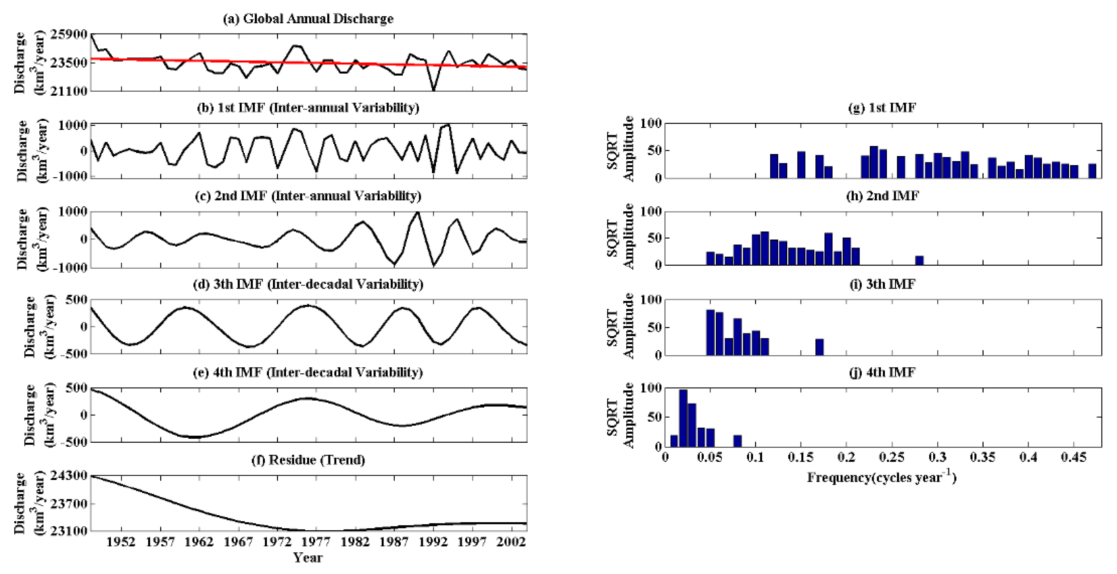
Using the total discharge from 925 river basins to approximate the global river discharge, we decomposed the global discharge time series into four IMFs and one trend component using EEMD (see Figure 1). The first IMF mode had a wide spectrum and represented synoptic oscillations with periods ranging from 2 years (1/0.47) to 8 years (1/0.12) (see Figure 1g). The second IMF represented variance with periods from 5 years (1/0.2) to 20 years (1/0.05) and centered at around 9 years (see Figure 1h). The third IMF contained mostly interdecadal variations with periods between 9years (1/0.11) and 20 years (1/0.05) (see Figure 1i). The 20 year to 50 year interdecadal variations were mostly captured by the fourth IMF (see Figure 1j). The differences between original time series and the sums of all four IMFs represented the trend (see Figure 1f).

Results from Figure 1f show that global river discharge decreased from 1948 to 1978, and then increased after 1978. This contrasts the result of no significant trend as estimated by the MK method that imposes a linear fit to a nonlinear trend (see Figure 1a). The estimated trend using the EEMD method in this study is consistent with previous studies that found significant shifts in global discharge trend around the 1970s from 1901 to 2002 [1,32,33].

Another advantage of EEMD is its ability to quantify the contribution of variance at different timescales to total variance of the observed time series. Using the results in Figure 1, we estimated that variance contributions were 41%, 25%, 10%, 9%, and 15% from the first, second, third, and fourth IMFs and the trend. The greater contribution by the trend than the third and fourth IMFs also suggests that the trend was nonlinear.

3.2. Spatial and Temporal Variation of River Discharge Trend from 1948 to 2004

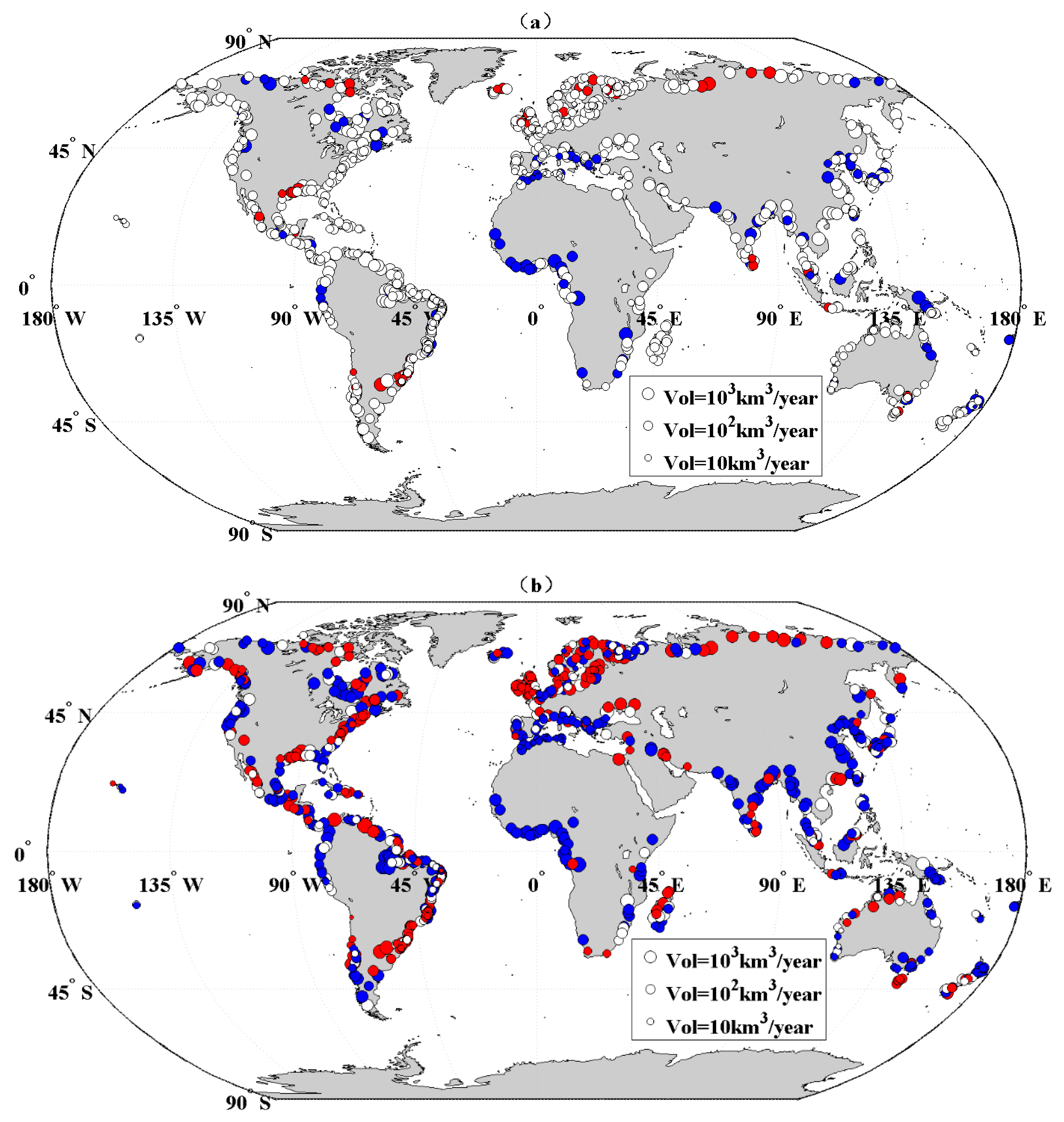
We compared the estimated trends by EEMD with those by MK for all 925 rivers. Consistent with the estimates by Dai et al. [6], our results using the MK approach showed that the discharge of about 80% of 925 rivers had no significant trends from 1948 to 2004, and that the number of rivers with significantly downward trends (116) was about twice as many as the number of rivers with significantly upward trends (48) (see Figure 2a). Contrary to the estimated trends using the MK method, estimates using EEMD showed that more than 70% of 925 rivers had significant trends from 1948–2004, including 292 of them with significantly upward trends in the regions of northern high latitudes, southeast North America, and southeast South America. Among those 70% rivers with significant trends, 442 of them had significantly downward trends, mainly in low latitudes. Only 191 rivers did not have significant trends from 1948–2004 (see Figure 2b). Because all discharge time series were not stationary, the trends estimated using MK method were not reliable. Our results are consistent with Nohara et al. [34] who found significant increases in the discharge of rivers in the northern high-latitude regions because of the increased precipitation. The downward trends for rivers in the subtropics found in this study are also consistent with Sun et al. [35] and Solomon et al. [36].

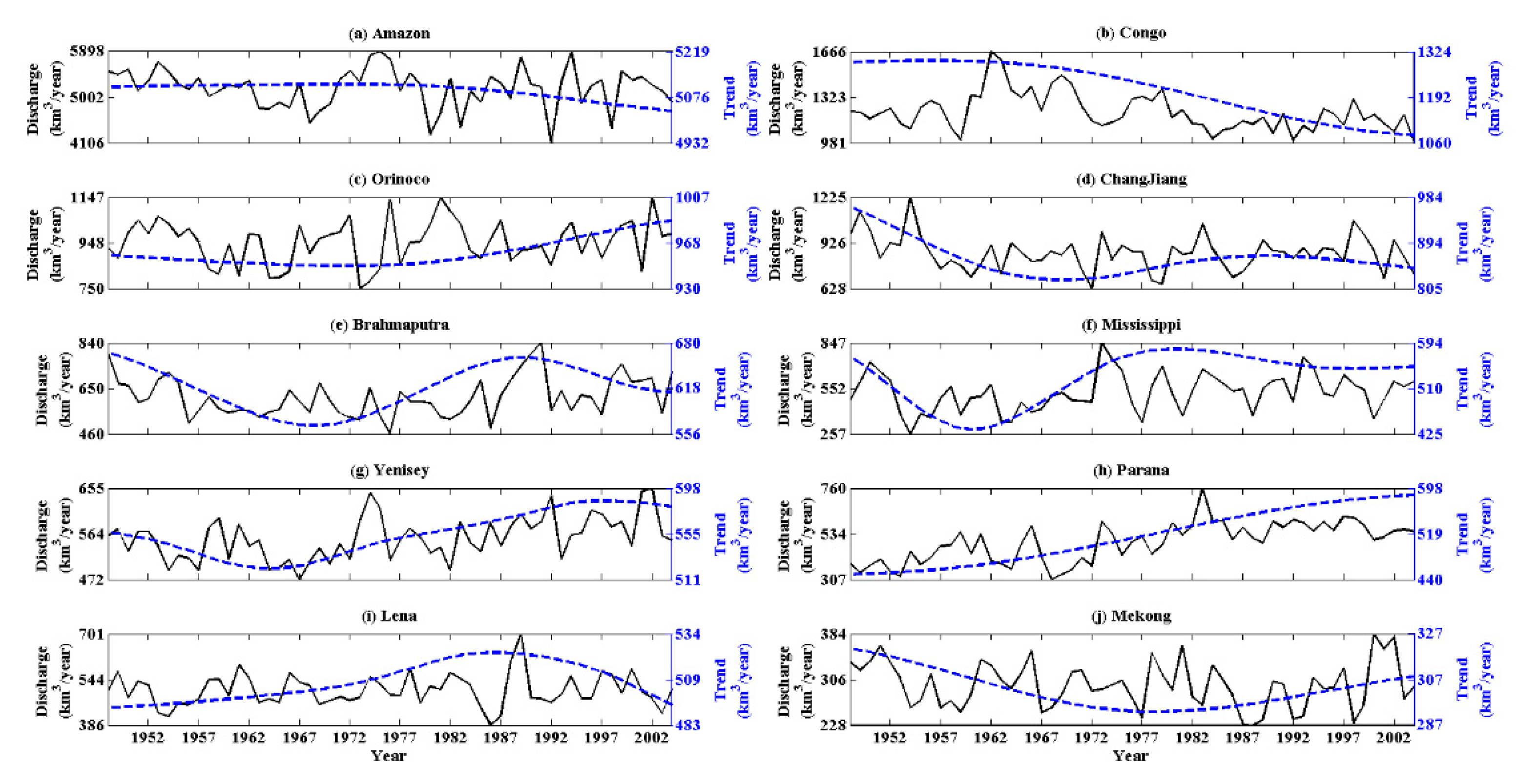
We also analyzed the temporal variations of the trends of all 925 river discharges and found that the trends of all river discharges were nonlinear over time. Figure 3 shows the annual mean discharge and its long-term trend using the EEMD method for the 10 largest rivers (sorted by annual mean volume) in the world. Results show that, for each river, that EEMD estimated a nonlinear trend, while the MK test gave nonsignificant trends for all 10 rivers except for river Congo with a significant downward trend and rivers Yenisey and Parana with significant upward trends (see Table S1, Supplementary Materials). Because of their trends being nonlinear over time, particularly for those rivers with a variable direction of change in the trend, the linear method is likely to give erroneous estimates.

3.3. Influences of Changing Trend and Variance of P and T on the Trend and Variance of River Discharge

Both theoretical studies and observations show that P and T likely influence variation and trend of river discharge [5], in addition to surface properties, such as vegetation and soil types, leaf area index, and so on. Here, we separately analyzed the correlations of detrended P or T with the detrended discharge or correlations of their respective trends. Figures S3 and S4 (Supplementary Materials) show the two global P products and two global T products we used in this study and their long-term trend computed by the EEMD method.

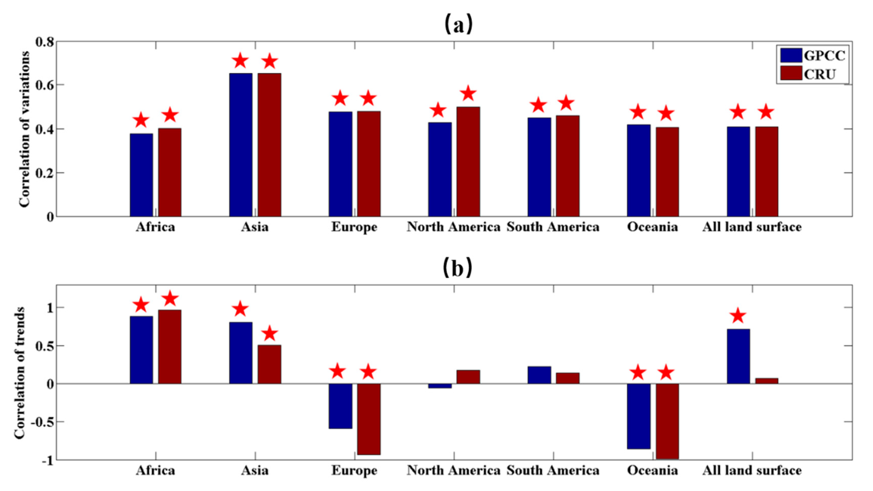
Because of the likely regional variations in discharge sensitivities to P or T variations, we grouped the discharge data, P and T, into six major continents or globally for correlation analysis. Across six continents or globally, variations in the detrended P and the detrended discharge time series were significantly and positively correlated, with the highest correlation valued about 0.7 for the Asian continent (see Figure 4). These correlations varied very little between the two different precipitation data products. However, correlations between the trends of P and discharge varied across different continents, being significantly positive for the African and Asian continents, significantly negative for the European and Oceanian continents, and not significant for the North American and South American continents. Correlations in the trends between discharge and P also differed between the two precipitation data products, being significantly positive for GPCC rainfall on a global scale, but insignificantly different from zero for the CRU TS4.0 data product on a global scale, suggesting relatively large uncertainties in the correlations of trends.

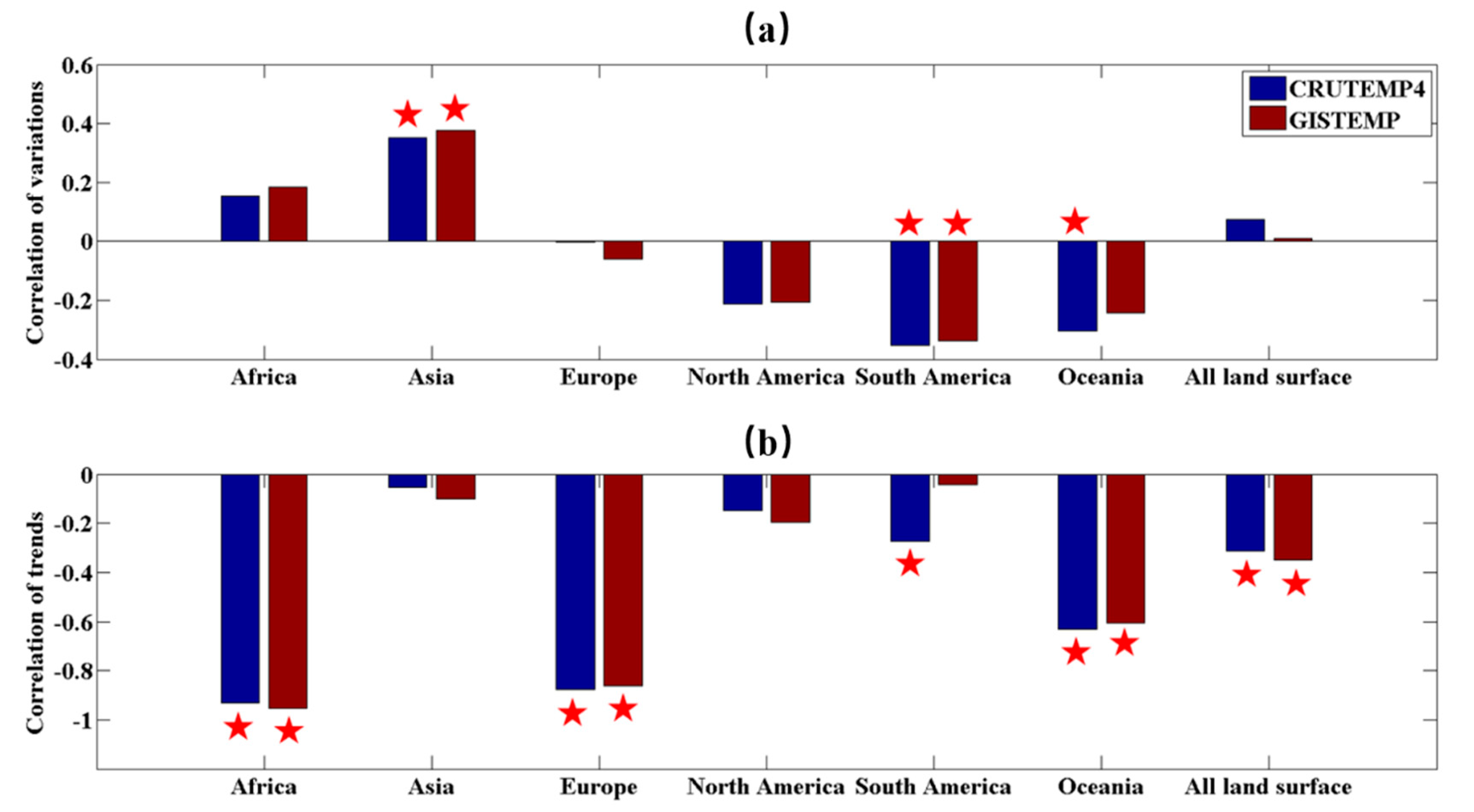
We also correlated the detrended and trend of discharge time series with two different products of global T. Correlations between the two detrended time series of discharge and T varied from region to region, being positive for African and Asian continents and negative for the other four continents. The correlation was only significant for Asia and South America for both products and Oceania for the CRUTEMP4 product. Globally, the detrended discharge was not significantly correlated with the detrended T for both temperature products (see Figure 5a). For the trends, T was negatively correlated with discharge across all six continents, and the correlation was only significant for Africa, Europe, and Oceania for both T products and South America for the CRUTEMP4 product (see Figure 5b). Globally, the trends of T and discharge were also significantly negatively correlated (see Figure 5b).

3.4. Sensitivity of the Estimated Global Continental Discharge to the Length of Data Record

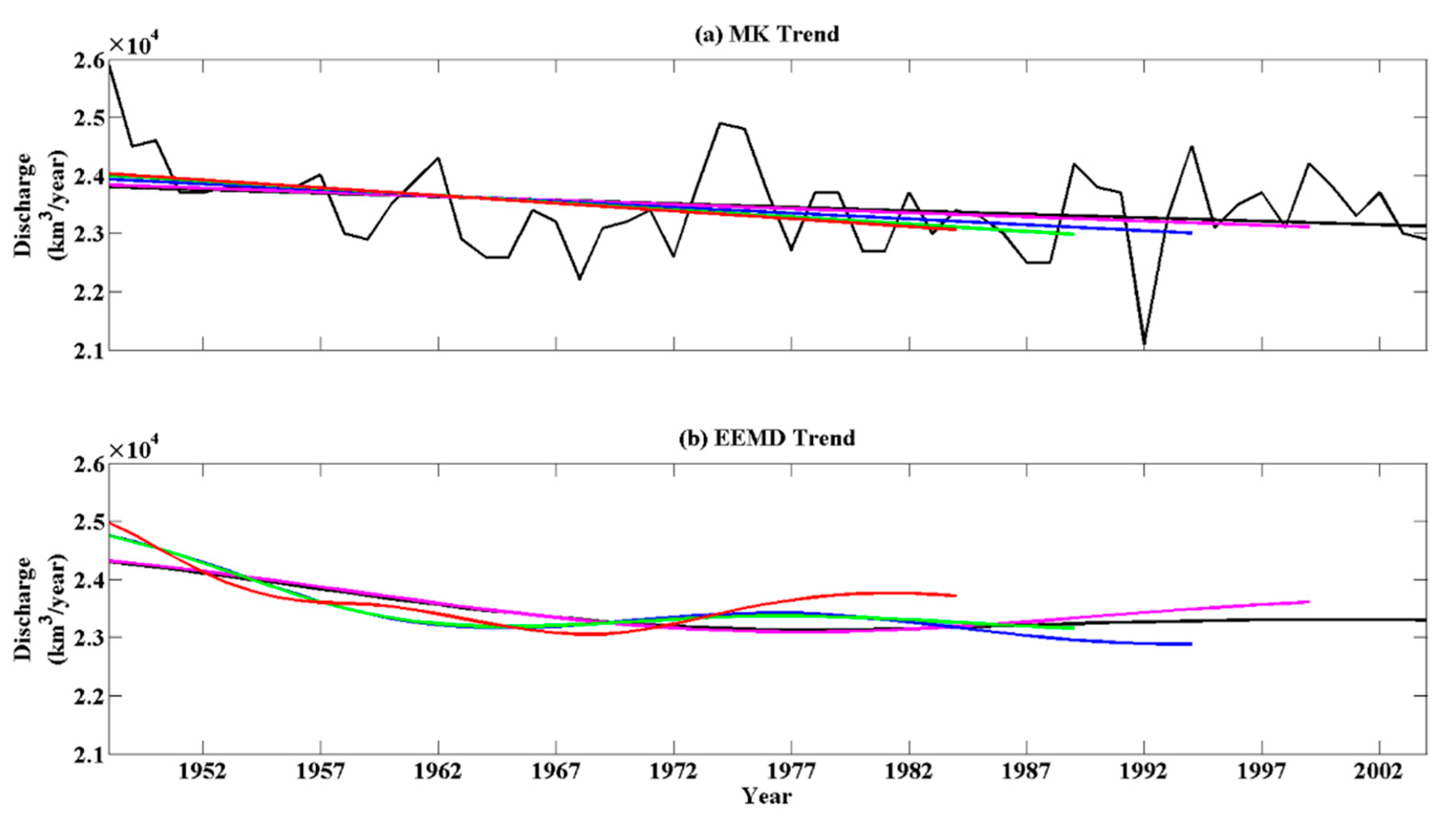
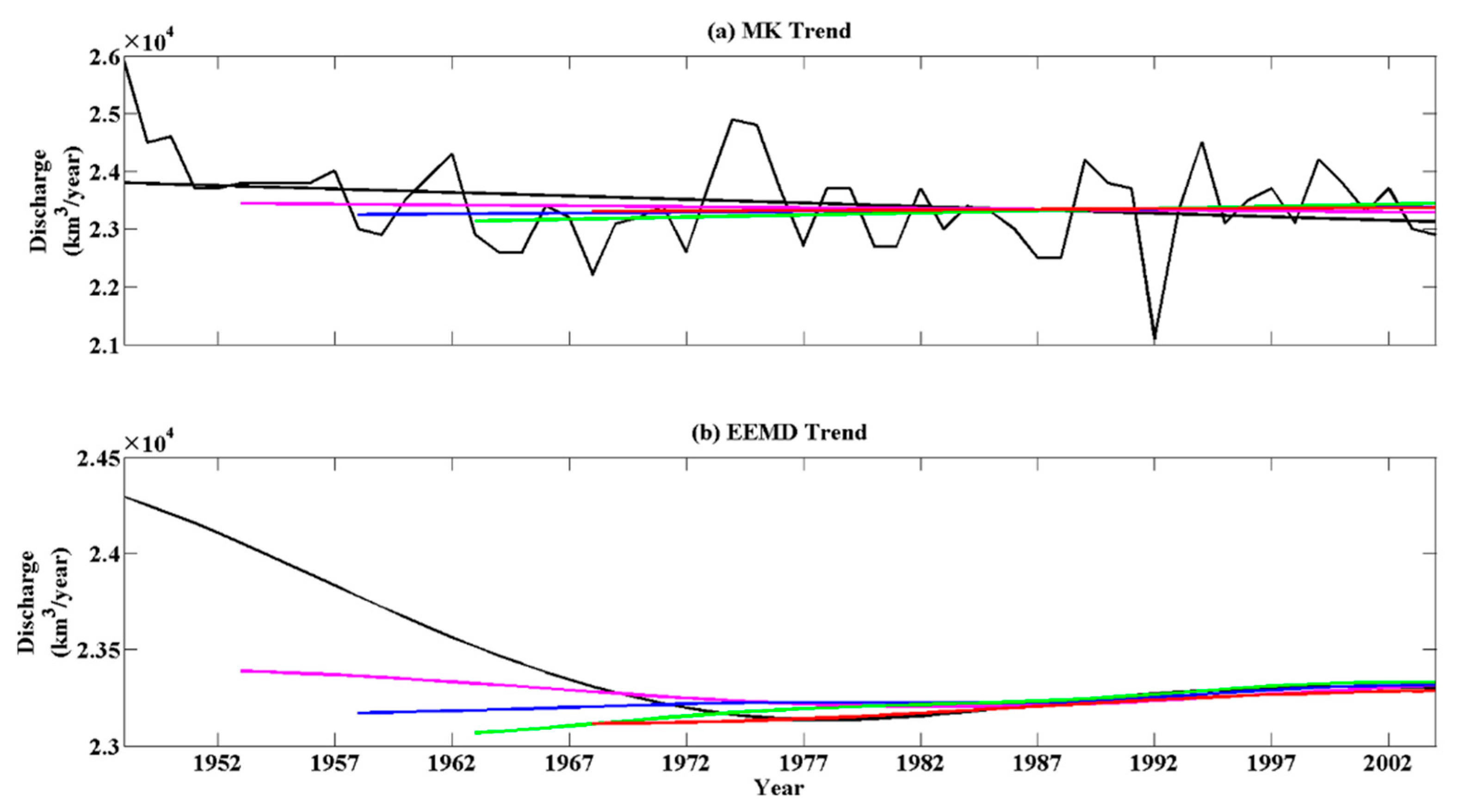
The estimated trend by EEMD can be sensitive to the data length. We compared the estimated trends using MK or EEMD methods for Dai’s global discharge data series with different ending and starting times (see Figure 6 and Figure 7). The discharge data included three periods with very high or low discharge rates, e.g., very high rates from 1948 to 1951 and from 1974 to 1975, and very low rates in 1992. The results in Figure 6 show that the estimated trends using the MK method were rather insensitive to the ending year. Depending on whether the two periods of very high (1974–1975) or low discharge (1992) were included or not, the trend estimated using EEMD could go up (see the red curve in Figure 6b) or down (see the blue curve in Figure 6b). Different sensitivities for the starting year of the estimated trends using the two methods are further illustrated in Figure 7. Overall, the linear trends as estimated using the MK method were not significantly different from zero. However, the estimated trend using the EEMD method could vary significantly, depending on whether the very high discharge period (1948–1951) was included or not. Only when the observed discharges of 1948–1951 were included, the trend in global discharge as estimated using the EEMD method decreased from 1948 to 1978 and then increased. The abnormally high discharge from 1948 to 1952 resulted in the global discharge time series being nonstationary with a nonlinear trend. This nonlinear trend was more accurately quantified using EEMD than using the MK method.

4. Discussion

The EEMD method presented here showed its advantage in dealing with nonstationary time series with a nonlinear trend. As the widely used MK method for trend quantification assumes stationarity, it is not strictly applicable to nonstationary time series such as river discharge. This study found that the MK method significantly underestimated the number of world’s major rivers with significant trends and the trends themselves, as compared with the EEMD method.

At a regional scale, contrary to the estimated trend of the MK method, estimates using EEMD showed that more than 70% of 925 rivers had significant trends from 1948–2004. The rivers with significantly upward trends were mainly located in the regions of northern high latitudes, southeast North America, and southeast South America, while those with significantly downward trends were mainly located in low latitudes. The decrease in precipitation over low- and mid-latitude areas and the increase in precipitation at high latitudes may have been the major cause for the change in river discharge over those different regions from 1948–2004 [6,37].

The observed great warming at high latitudes may have also contributed to the observed increase in discharge in those regions. Nijssen et al. [38] found that the predicted warming in high-latitude basins was greatest during the winter months, which may lead to the stored snow melting as stream flow. The rising temperature also results in increases in oceanic evaporation and, consequently, increased precipitation and runoff over land [6]. Furthermore, surface warming at high latitudes has caused a degradation of the permafrost, which may also contribute to increases in discharge trend at these latitudes [12]. As a result, this leads to the hypothesis that there will be an intensification of the global water cycle, especially at high latitudes [5]. However, our study showed that the process may be more complex because the climate system is highly nonlinear. The effect of climate change on global water cycle also exhibits some nonlinearities.

More importantly our analysis showed that variations in precipitation had dominant influences on the variances in river discharge both regionally and globally, while the trends of discharge might be influenced by many other factors, including atmospheric CO₂, land-use change, and climate change [33,39,40]. This means that the variation in continental discharge is mainly caused by climate variance, while the causes of the change in discharge trend are more difficult to identify. However, correctly quantifying the observed trend of regional or global discharge is a prerequisite. Because of large regional and temporal variations in the trends of the observed river discharges, attribution studies of discharge trend should focus on different regions using global land models, such as those by Gedney et al. [39] and Piao et al. [40].

The estimated change in the trend of global river discharge around 1978 had significant implications for our interpretation of how various external factors influenced the global hydrological cycle over time. Globally, the river discharge decreased before 1978 and increased after 1978, while global surface temperature increased steadily over the study period, which is different from the estimated sensitivity by Labat et al. [5] showing that the river runoff is increasing with global warming. According to the increasing trend of global discharge as estimated by Labat et al. [5] using the MK method, Gedney et al. [39] attributed the decrease in evapotranspiration to increasing atmospheric CO₂ as the dominant cause, while land-use changes, climate change, or increased precipitation were considered as the major causes by other studies [33,40]. If the trend differs in direction before and after 1978, the claim highlighting increasing CO₂ alone as the likely cause is unlikely to hold [41]. Future studies should focus on why the trend changed from a downward trend before 1978 to a small upward trend after 1978.

Because the trend of global river discharge is nonlinear, the estimated trend can be affected by the uncertainties and lengths of the observed datasets [10]. This study also showed that the estimated trend of global river discharge from 1948 to 2004 using EEMD was very sensitive to the unusually high discharge rate in the first 4 years. The difference in the estimated trend of global river discharge between the previous two studies by Labat et al. [5] and Dai et al. [6] may have resulted from the different amount of data (221 vs. 925 rivers) and different period (the whole 20th century vs. 1948 to 2004). Therefore, it is important to compare the estimated trend for the same period.

Water demands (especially for irrigation systems) are also a factor that influence the continental discharge trend. To demonstrate this kind of effect, we used the Global Map of Irrigation Areas (GMIA) version 5 (http://www.fao.org/nr/water/aquastat/irrigationmap/index10.stm) from the Food and Agriculture Organization (FAO) of the United Nations to show whether irrigation had a significant effect on continental discharge trend (Figure S5, Supplementary Materials). At the global scale, northern India and the North China Plain are the most intensive irrigation areas, while others have very low percentages of irrigation practices (Figure S5a, Supplementary Materials). However, these two places mainly used groundwater to irrigate (Figure S5c, Supplementary Materials). We concluded that irrigation may have little effect on the global continental discharge trend. In this study, we did not conclude irrigation as one of the impact factors on the global continental discharge trend. Our result is consistent with Haddeland et al. [42], who found that the impact of manmade reservoirs and water withdrawals on the long-term global terrestrial water balance was small.

Our results have other implications, e.g., they provided a new idea to better quantify model simulation uncertainties. Land surface and hydrological models always simulate gridded runoff [43]. The model-simulated runoff may contain significant bias due to errors in the meteorological forcing data and model structure. However, runoff is difficult to measure directly, while discharge over most of the world’s major rivers has been monitored by stream gauges for many decades [6]. Thus, historical records of discharge provide a measure of basin-integrated runoff, and they have been used to calibrate model-simulated runoff field. Nevertheless, it is difficult for models to fully simulate the long-term time series of runoff/discharge. If the models can exactly simulate the long-term trend of runoff/discharge, they will also be of great reference value. Accurately identifying the discharge trend is the basis of the abovementioned model evaluations. In the future, it is necessary for model developers to not only reduce the uncertainties of time series modeled discharge, but also to accurately simulate the nonlinear discharge trend.

Our study also has implications for guiding future water use in people’s production and life. The global water cycle is expected to change over the 21st century due to the combined effects of climate change and increasing human activities. In a warm world, the water holding capacity of the atmosphere will increase, resulting in a change in the frequency of extreme events, e.g., precipitation extremes and dry periods. Under the moderate representative concentration pathway (RCP) 4.5 emissions scenario, annual precipitation could increase by 10–25% from 1970–1999 to 2070–2099 over most of Eurasia, North America, and central to northern Africa, but decrease by 3–15% over most of Australia, southern Africa, and Central America [6]. The changes in future precipitation will greatly affect the trends of continent discharge. On the basis of the accurate calculation of global and regional discharge trends, we can apply quantitative attribution analysis to the trend results. The attribution results can demonstrate which are the key determinants of nonlinear discharge trends [39,40] and help us understand the physical mechanism of water cycle under the influence of climate change and human activities. These results can be used to construct a new model or improve the existing models to predict the shortage of water resources under the future climate change scenarios, which in turn can provide valuable references for water resource management policies. For example, if we predict significant downward discharge trends at some point in the future in one or more watersheds, long-term planning for water resources can be prepared in advance in order to guarantee domestic and agricultural water. Thus, an accurate calculation of discharge trend has momentous application values to the guidance of water use in people’s production and life.

Our study had some limitations. For example, the calculation results deeply depended on whether there were sufficient discharge data. Our calculation of discharge trend required complete time-series data. However, in actual observations, especially for long-time-scale data, there is often a lack of measurements. In this paper, we used Dai’s discharge data which were compiled and gap-filled by many technical means, including CLM3 model simulation and others. The final dataset met our requirements to compute the long-term discharge trend. However, Dai’s dataset was populated at the farthest downstream stations for the major rivers. According to this dataset, we could not test if the discharge trends changed in one river’s upstream and downstream gauge sections. If more discharge observations can be acquired in the future, we should conduct more analysis to show what happens for a river’s different gauge stations.

5. Conclusions

In this study, we performed discharge trend analysis of 925 global rivers in the period from 1948–2004 using the EEMD method. Results showed that the EEMD method can better estimate the nonlinear and nonstationary nature of discharge trends at a global and regional scale, compared with the commonly used MK method. At a global scale, the EEMD method showed that the continental discharge trend decreased before 1978 and increased after 1978 in the period from 1948 to 2004, whereas the commonly used MK method gave no significant trend along the data span. At a regional scale, the EEMD method estimated that more than 70% of the 925 rivers had significant trends, including 292 of them with significantly upward trends and the others with significantly downward trends. On the other hand, the MK method consistently underestimated the discharge trends. We strongly recommend that future studies should adopt EEMD for analyzing the nonlinear trends of all hydrological nonstationary time series and perhaps all geophysical nonstationary time series.

We also found that precipitation had consistently dominant influences on the variations in discharge across six continents and globally, but the influencing factors of discharge trend were more complex. Future studies should particularly focus on explaining why the global runoff trend changed direction around 1978 using process-based global land or hydrological models.

References

- Milly, P.C.; Dunne, K.A.; Vecchia, A.V. Global pattern of trends in streamflow and water availability in a changing climate. Nature 2005, 438, 347–350. [Google Scholar] [CrossRef] [PubMed]
- Oki, T.; Kanae, S. Global hydrological cycles and world water resources. Science 2006, 313, 1068. [Google Scholar] [CrossRef] [PubMed] [Green Version]
- Betts, R.A.; Boucher, O.; Collins, M.; Cox, P.M.; Falloon, P.D.; Gedney, N.; Hemming, D.L.; Huntingford, C.; Jones, C.D.; Sexton, D.M.H.; et al. Projected increase in continental runoff due to plant responses to increasing carbon dioxide. Nature 2007, 448, 1037–1041. [Google Scholar] [CrossRef]
- Milly, P.C.; Betancourt, J.; Falkenmark, M.; Hirsch, R.M.; Kundzewicz, Z.W.; Lettenmaier, D.P.; Stouffer, R.J. Stationarity is dead: Whither water management? Science 2008, 319, 573–574. [Google Scholar] [CrossRef] [PubMed]
- Labat, D.; Goddéris, Y.; Probst, J.L.; Guyot, J.L. Evidence for global runoff increase related to climate warming. Adv. Water Resour. 2004, 27, 631–642. [Google Scholar] [CrossRef]
- Dai, A.; Qian, T.; Trenberth, K.E.; Milliman, J.D. Changes in continental freshwater discharge from 1948–2004. J. Clim. 2009, 22, 2773. [Google Scholar] [CrossRef]
- Alkama, R.; Kageyama, M.; Ramstein, G. Relative contributions of climate change, stomatal closure, and leaf area index changes to 20th and 21st century runoff change: A modelling approach using the organizing carbon and hydrology in dynamic ecosystems (ORCHIDEE) land surface model. J. Geophys. Res. Atmos. 2010, 115, D17112. [Google Scholar] [CrossRef]
- Alkama, R.; Marchand, L.; Ribes, A.; Decharme, B. Detection of global runoff changes: Results from observations and CMIP5 experiments. Hydrol. Earth Syst. Sci. 2013, 17, 2967–2979. [Google Scholar] [CrossRef] [Green Version]
- Legates, D.R.; Lins, H.F.; McCabe, G.J. Comments on “Evidence for global runoff increase related to climate warming” by Labat et al. Adv. Water Resour. 2005, 28, 1310–1315. [Google Scholar] [CrossRef]
- Peel, M.C.; McMahon, T.A. Recent frequency component changes in interannual climate variability. Geophys. Res. Lett. 2006, 33, 373–386. [Google Scholar] [CrossRef]
- Milliman, J.D.; Farnsworth, K.L.; Jones, P.D.; Xu, K.H.; Smith, L.C. Climatic and anthropogenic factors affecting river discharge to the global ocean, 1951–2000. Glob. Planet. Chang. 2008, 62, 187–194. [Google Scholar] [CrossRef]
- Alkama, R.; Decharme, B.; Douville, H.; Ribes, A. Trends in global and basin-scale runoff over the late twentieth century: Methodological issues and sources of uncertainty. J. Clim. 2011, 24, 3000–3014. [Google Scholar] [CrossRef]
- Sang, Y.F.; Wang, Z.; Liu, C. Comparison of the MK test and EMD method for trend identification in hydrological time series. J. Hydrol. 2014, 510, 293–298. [Google Scholar] [CrossRef]
- Wu, Z.; Huang, N.E.; Long, S.R.; Peng, C.K. On the trend, detrending, and variability of nonlinear and nonstationary time series. Proc. Natl. Acad. Sci. USA 2007, 104, 14889. [Google Scholar] [CrossRef] [PubMed] [Green Version]
- Mann, H.B. Nonparametric tests against trend. Econometrica 1945, 13, 245–259. [Google Scholar] [CrossRef]
- Kendall, M.G. Rank Correlation Methods; Charles Grifin: London, UK, 1975. [Google Scholar]
- Yue, S.; Pilon, P.; Cavadias, G. Power of the Mann–Kendall and Spearman’s rho tests for detecting monotonic trends in hydrological series. J. Hydrol. 2002, 259, 254–271. [Google Scholar] [CrossRef]
- Hamed, K.H. Trend detection in hydrologic data: The Mann–Kendall trend test under the scaling hypothesis. J. Hydrol. 2008, 349, 350–363. [Google Scholar] [CrossRef]
- Sun, F.; Roderick, M.L.; Farquhar, G.D. Rainfall statistics, stationarity, and climate change. Proc. Natl. Acad. Sci. USA 2018, 115, 2305–2310. [Google Scholar] [CrossRef] [Green Version]
- Hamed, K.H.; Rao, A.R. A modified Mann-Kendall trend test for autocorrelated data. J. Hydrol. 1998, 204, 192–196. [Google Scholar] [CrossRef]
- Su, L.; Miao, C.; Kong, D.; Duan, Q.; Lei, X.; Hou, Q.; Li, H. Long-term trends in global river flow and the causal relationships between river flow and ocean signals. J. Hydrol. 2018, 563, 818–833. [Google Scholar] [CrossRef]
- Hurst, H.E. Long-term storage capacity of reservoirs. Trans. Am. Soc. Civ. Eng. 1951, 116, 770–799. [Google Scholar] [CrossRef]
- Huang, N.E.; Shen, Z.; Long, S.R.; Wu, M.C.; Shih, H.H.; Zheng, Q.; Yen, N.; Tung, C.C.; Liu, H.H. The Empirical Mode Decomposition Method and the Hilbert Spectrum for Non-stationary Time Series Analysis. Proc. R. Soc. Lond. A 1998, 454, 903–995. [Google Scholar] [CrossRef]
- Huang, N.E.; Shen, Z.; Long, S.R. A new view of nonlinear water waves: The Hilbert spectrum. Annu. Rev. Fluid Mech. 1999, 31, 417–457. [Google Scholar] [CrossRef] [Green Version]
- Chen, X.; Zhang, X.; Church, J.A.; Watson, C.S.; King, M.A.; Monselesan, D.; Legresy, B.; Harig, C. The increasing rate of global mean sea-level rise during 1993–2014. Nat. Clim. Chang. 2017, 7, 492–497. [Google Scholar] [CrossRef]
- Ji, F.; Wu, Z.; Huang, J.; Chassignet, E.P. Evolution of land surface air temperature trend. Nat. Clim. Chang. 2014, 4, 462–466. [Google Scholar] [CrossRef]
- Pan, N.; Feng, X.; Fu, B.; Wang, S.; Ji, F.; Pan, S. Increasing global vegetation browning hidden in overall vegetation greening: Insights from time-varying trends. Remote Sens. Environ. 2018, 214, 59–72. [Google Scholar] [CrossRef]
- Mhamdi, F.; Poggi, J.M.; Jaïdane, M. Trend extraction for seasonal time series using ensemble empirical mode decomposition. Adv. Data Anal. 2011, 3, 363–383. [Google Scholar] [CrossRef]
- Carmona, A.M.; Poveda, G. Detection of long-term trends in monthly hydro-climatic series of Colombia through Empirical Mode Decomposition. Clim. Chang. 2014, 123, 301–313. [Google Scholar] [CrossRef]
- Jones, P.D.; New, M.G.; Parker, D.E.; Marun, S.; Rigor, I.G. Surface air temperature and its changes over the past 150 years. Rev. Geophys. 1999, 37, 173–199. [Google Scholar] [CrossRef]
- Hansen, J.; Ruedy, R.; Glascoe, J.; Sato, M. GISS analysis of surface temperature change. J. Geophys. Res. 1999, 104, 30997–31022. [Google Scholar] [CrossRef]
- Krakauer, N.Y.; Fung, I. Mapping and attribution of change in streamflow in the coterminous united states. Hydrol. Earth Syst. Sci. 2008, 12, 1111–1120. [Google Scholar] [CrossRef] [Green Version]
- Gerten, D.; Rost, S.; von Bloh, W.; Lucht, W. Causes of change in 20th century global river discharge. Geophys. Res. Lett. 2008, 35, L20405. [Google Scholar] [CrossRef]
- Nohara, D.; Kitoh, A.; Hosaka, M.; Oki, T. Impact of climate change on river discharge projected by multimodel ensemble. J. Hydrometeorol. 2006, 7, 1076. [Google Scholar] [CrossRef] [Green Version]
- Sun, Y.; Solomon, S.; Dai, A.; Portmann, R.W. How often will it rain? J. Clim. 2007, 20, 4801–4818. [Google Scholar] [CrossRef]
- Solomon, S.; Qin, D.; Manning, M.; Marquis, M.; Averyt, K.; Tignor, M.M.B.; Miller, H.L., Jr.; Chen, Z. (Eds.) Climate Change 2007: The Physical Science Basis; Cambridge University Press: Cambridge, UK, 2007; p. 996. [Google Scholar] [CrossRef] [Green Version]
- Mccabe, G.J.; Wolock, D.M. Century-scale variability in global annual runoff examined using a water balance model. Int. J. Clim. 2011, 31, 1739–1748. [Google Scholar] [CrossRef]
- Nijssen, B.; O’Donnell, G.M.; Hamlet, A.F.; Lettenmaier, D.P. Hydrologic sensitivity of global rivers to climate change. Clim. Chang. 2001, 50, 143–175. [Google Scholar] [CrossRef]
- Gedney, N.; Cox, P.M.; Betts, R.A.; Boucher, O.; Huntingford, C.; Stott, P.A. Detection of a direct carbon dioxide effect in continental river runoff records. Nature 2006, 439, 835–838. [Google Scholar] [CrossRef]
- Piao, S.; Friedlingstein, P.; Ciais, P.; Nobletducoudré, N.D.; Labat, D.; Zaehle, S. Changes in climate and land use have a larger direct impact than rising CO2 on global river runoff trends. Proc. Natl. Acad. Sci. USA 2007, 104, 15242. [Google Scholar] [CrossRef] [Green Version]
- Franzke, C.L.E.; O’Kane, T.J.; Monselesan, D.P.; Risbey, J.S.; Horenko, I. Systematic attribution of observed Southern Hemisphere circulation trends to external forcing and internal variability. Nonlinear Process. Geophys. 2015, 2, 675–707. [Google Scholar] [CrossRef]
- Haddeland, I.; Heinke, J.; Biemans, H.; Eisner, S.; Flörke, M.; Hanasaki, N.; Konzmann, M.; Ludwig, F.; Masaki, Y.; Schewe, J.; et al. Global water resources affected by human interventions and climate change. Proc. Natl. Acad. Sci. USA 2014, 111, 3251–3256. [Google Scholar] [CrossRef] [Green Version]
- Lawrence, D.M.; Oleson, K.W.; Flanner, M.G.; Thornton, P.E.; Swenson, S.C.; Lawrence, P.J.; Zeng, X.; Yang, Z.-L.; Levis, S.; Sakaguchi, K.; et al. Parameterization improvements and functional and structural advances in version 4 of the Community Land Model. J. Adv. Model. Earth Syst. 2011, 3, 365–375. [Google Scholar] [CrossRef]
Figure 1.
Annual global freshwater discharge from 1948 to 2004 (a), and its decomposition into four intrinsic mode functions (b–e) and trend (f) using ensemble empirical mode decomposition (EEMD). The red line in (a) represents the trend estimate using the Mann–Kendall (MK) method, and the power spectrum of each intrinsic mode function (IMF) is also shown in (g–j).
Figure 2.
Trends of 925 river discharges to the ocean from 1948–2004 as estimated using MK (a) or EEMD (b) methods. Stations with significant upward (downward) trends are shown in red (blue), while white circles represent no significant trend. The log transform of annual volume discharge is proportional to the area of each circle, and each circle is located at the mouth of the watershed.
Figure 3.
The constructed discharge time series of the 10 largest rivers (black curve) and their trends (blue curve) as estimated using the EEMD method from 1948–2004.
Figure 4.
Correlations of (a) the detrended time series of annual precipitation and discharge from 1948 to 2004; (b) the trends of precipitation and discharge from 1948 to 2004; the red star represents significant correlation at the 95% level.
Figure 5.
Same as Figure 4 but for the correlations between (a) the detrended time series of annual surface air temperature and discharge from 1948 to 2004; (b) the trends of surface air temperature and discharge from 1948 to 2004; the red star represents significant correlation at the 95% level.
Figure 6.
Sensitivity of the estimated trends to the same starting year (1948) but different ending year of global runoff data. Different colors represent the estimated trends for ending times of 1979, 1984, 1989, 1994, 1999, and 2004. The estimated trends are shown in (a) for the MK method and (b) for the EEMD method.
Figure 7.
Same as Figure 6, but the trends calculated based on global discharge data with the same ending time (2004), but different starting years of 1948, 1953, 1958, 1963, 1968, and 1973. The estimated trends are shown in (a) for the MK method and (b) for the EEMD method.
Publisher’s Note: MDPI stays neutral with regard to jurisdictional claims in published maps and institutional affiliations. |
© 2020 by the authors. Licensee MDPI, Basel, Switzerland. This article is an open access article distributed under the terms and conditions of the Creative Commons Attribution (CC BY) license (http://creativecommons.org/licenses/by/4.0/).
Share and Cite
MDPI and ACS Style
Wang, C.; Zhang, H. Trend and Variance of Continental Fresh Water Discharge over the Last Six Decades. Water 2020, 12, 3556. https://doi.org/10.3390/w12123556
AMA Style
Wang C, Zhang H. Trend and Variance of Continental Fresh Water Discharge over the Last Six Decades. Water. 2020; 12(12):3556. https://doi.org/10.3390/w12123556
Chicago/Turabian StyleWang, Chen, and Hui Zhang. 2020. "Trend and Variance of Continental Fresh Water Discharge over the Last Six Decades" Water 12, no. 12: 3556. https://doi.org/10.3390/w12123556
Note that from the first issue of 2016, this journal uses article numbers instead of page numbers. See further details here.