Changing Low Flow and Streamflow Drought Seasonality in Central European Headwaters

Abstract

In the context of the ongoing climate warming in Europe, the seasonality and magnitudes of low flows and streamflow droughts are expected to change in the future. Increasing temperature and evaporation rates, stagnating precipitation amounts and decreasing snow cover will probably further intensify the summer streamflow deficits. This study analyzed the long-term variability and seasonality of low flows and streamflow droughts in fifteen headwater catchments of three regions within Central Europe. To quantify the changes in the low flow regime of selected catchments during the 1968–2019 period, we applied the R package lfstat for computing the seasonality ratio (SR), the seasonality index (SI), mean annual minima, as well as for the detection of streamflow drought events along with deficit volumes. Trend analysis of summer minimum discharges was performed using the Mann–Kendall test. Our results showed a substantial increase in the proportion of summer low flows during the analyzed period, accompanied with an apparent shift in the average date of low flow occurrence towards the start of the year. The most pronounced seasonality shifts were found predominantly in catchments with the mean altitude 800–1000 m.a.s.l. in all study regions. In contrast, the regime of low flows in catchments with terrain above 1000 m.a.s.l. remained nearly stable throughout the 1968–2019 period. Moreover, the analysis of mean summer minimum discharges indicated a much-diversified pattern in behavior of long-term trends than it might have been expected. The findings of this study may help identify the potentially most vulnerable near-natural headwater catchments facing worsening summer water scarcity.

1. Introduction

Regional and local hydrological studies are of high importance because they present both spatial and temporal variability of runoff characteristics, although on a relatively small scale [1,2]. The assessment of the streamflow extremes on a local scale should begin with the identification of typical seasonal variations occurring over time [3]. Due to the changing climate, these patterns may be either aggravating or weakening throughout a longer period of time [4,5].

The increasing frequency, intensity and duration of streamflow droughts in mid-latitudes of the Northern Hemisphere represent some of the predicted effects of climate change [6,7,8]. In the context of increasing severity of droughts in Europe during the last decade [9,10,11], the effects of climate change on runoff regime will very likely affect the runoff seasonality, variability of discharge and also the risk of extreme streamflow drought occurrence [12,13]. Under conditions of rising air temperature, increasing evaporation rates, decreasing soil-moisture [14,15,16] and decreasing snow cover in the Central European region [17,18,19], the droughts are more likely to occur and escalate into multiyear events.

The evidence suggests that severe droughts may cause particularly dangerous impacts for society, agriculture, ecosystems and water management if the events last more than one year and water resources cannot be completely recharged [20,21,22,23]. During such periods, the increased water demand could further intensify streamflow droughts, affecting negatively either low flows or deficit volumes [24]. Recent observations from Europe showed that many regions with a flow regime driven by rainfall, such as southern France, southwestern England or Central Europe will be prone to multiyear drought in the future [25]. In contrast, the catchments with a flow regime dominated by snowmelt should not be significantly affected by multiyear drought events, indicating an increasing divergence in the probability of drought occurrence across Europe [25,26]. However, there are also predictions of a significant decrease in summer low flows due to a shift in snowmelt season and overall decrease in snow water equivalent even for elevations around 1000 m.a.s.l. and higher [27].

The effect of climate change on low flows and their seasonality has also been a subject of recent European studies [28,29,30]. In many catchments of different scales in Central Europe, e.g., the Upper Rhine, the future shift from the winter low-flow regime to the summer low-flow regime is expected. Furthermore, the variability of low-flow event timing will also decrease with ongoing climate warming, which should make the droughts more predictable [31]. To understand the long-term behavior of the runoff changes in Central Europe, the observations from near-natural catchments are highly important [32]. The observed patterns from Central European headwaters might therefore provide valuable information for research in other regions.

The main aim of this study was to evaluate the long-term variability and seasonality of low flows and streamflow droughts in 15 headwater, near-natural catchments of five mountain ranges and highlands within the Central European region. With respect to the outputs of recent studies with similar interest reflecting consecutive warming, decreasing snow cover and relatively stable amounts of total precipitation in the Central European region [12,18,33,34], we hypothesized that (1) the ongoing climate change causes a significant change in the ratio between summer and winter low flows, which (2) affects the seasonal distribution of low flows and streamflow droughts in the study catchments, and that (3) the duration and magnitude of streamflow drought events are therefore increasing during the analyzed period.

To perform the analysis of low flow and streamflow drought characteristics in study catchments, we used a set of daily discharge data for the 1968–2019 period. The seasonality ratio (SR) was used to characterize the low-flow regime of the rivers, the seasonality index (SI) was derived to evaluate the average timing and concentration of low flows and streamflow droughts during the year. For each catchment, the durations of streamflow drought events along with the deficit volumes were derived. The Mann–Kendall nonparametric test together with Sen’s slope estimator were used to examine the significance and direction of trends in time series of seven- and 30-day mean summer minimum discharges (MSM-7; MSM-30).

To provide a detailed insight into the dynamics and evolution of low-flow and streamflow drought indices and characteristics in the study catchments during the evaluated period (1968–2019), we derived the 30-year moving averages for most of the low-flow and drought indices as well as for their trend properties. This approach allowed us to observe the recent variations and inner changes of the low-flow regime in selected Central European headwaters more closely and it also diminished the influence of short-term variations and outliers within the observation period. This research helps to explore the potentially most vulnerable, near-natural headwater catchments to the summer water scarcity in Central Europe.

2. Materials and Methods

2.1. Study Area

This study was performed in 15 headwater catchments in mountains and highlands along the Czech Republic’s border with Germany and Poland (Figure 1). Geographically, the study catchments were divided into three groups according to their location in order to better distinguish the intra- and inter-regional variability of the results according to their physiographic properties (

Table 1. Basic characteristics of study catchments. Data: CHMI, GKD Bayern, LfULG Sachsen.

Stream Gauge	Abbrev.	Stream	Region	Area (km2)	Stream Gauge Coordinates	Gauge Elevation (m.a.s.l.)	Mean Elevation (m.a.s.l.)	Mean Slope (°)	Dominant Hillslope Orientation
Blanicky Mlyn	BLA	Blanice	SW	85.47	48.957N 13.941E	743.42	897.1	5.72	N; NW
Kolinec	KOL	Ostruzna	SW	91.68	49.296N 13.436E	531.65	755.7	7.33	NE; N
Modrava	MOD	Vydra	SW	89.80	49.026N 13.497E	973.28	1146.6	5.42	NE; W
Höll	HOL	Schwarzach	SW	59.90	49.410N 12.704E	493.25	651.7	7.93	SW; W
Linden	LIN	Sausswasser	SW	89.70	48.825N 13.565E	649.74	899.2	7.81	SW; W
Lohberg	LOH	Weißer Regen	SW	39.30	49.172N 13.091E	575.76	927.5	13.27	SW; W
Klingenthal 1	KLI	Zwota	NW	55.70	50.354N 12.471E	540.10	719.7	8.89	SE; S
Chaloupky	CHA	Rolava	NW	20.06	50.374N 12.664E	804.62	907.1	3.95	S; SW
Rothenthal	ROT	Natzschung	NW	76.10	50.619N 13.360E	538.22	762.8	5.10	NE; N
Rehefeld 2	REH	Wilde Weißeritz	NW	15.40	50.728N 13.701E	685.45	805.6	5.93	W; NW
Ammelsdorf	AMM	Wilde Weißeritz	NW	49.30	50.805N 13.607E	527.37	734.4	7.12	NE; W
Janov–Harrachov	JAN	Mumlava	NE	51.31	50.765N 15.397E	580.65	978.7	11.08	SW; W
Dolni Stepanice	DOL	Jizerka	NE	44.08	50.638N 15.517E	441.51	860.3	13.88	SW; S
Horni Marsov	HOR	Upa	NE	81.99	50.661N 15.820E	570.45	1048.4	16.01	SE; E
Marsov n. Metuji	MAR	Metuje	NE	94.68	50.530N 16.190E	418.03	583.7	8.07	E; SE

). The regions were specified as follows:

• Southwest (SW): catchments of the Bohemian Forest (BLA, KOL, MOD) and the Bavarian Forest (HOL, LOH, LIN)
• Northwest (NW): catchments of the Ore Mountains (KLI, CHA, ROT, REH and AMM)
• Northeast (NE): catchments of the Giant Mountains (JAN, DOL, HOR) and the Broumov Highlands (MAR)

Twelve of the selected catchments belong to the Elbe River basin, while the remaining three catchments in the SW region (HOL, LOH and LIN) represent headwaters of the Danube tributaries. Generally, the study catchments were selected because of multiple necessary conditions:

• Availability of at least 50 years of daily streamflow time series;
• Absence of dams, large weirs or other structures significantly regulating streamflow;
• Areal and altitudinal properties (area <100 km², mean altitude >550 m.a.s.l.).

Although the catchments were chosen based on criteria of similarity, there are some variations in their physical and natural properties worth noting. According to the Köppen–Geiger climate classification, catchments with mean altitude above 850 m.a.s.l. belong to the Dfb category, while study catchments with lower average altitude are classified as Cfb [35]. Study catchments receive a relatively evenly distributed amount of annual precipitation that ranges from 800 to 1300 mm. Annual mean air temperatures vary between 2.5 and 8 °C, with respect to the altitude. All study catchments are located in mountains and highlands of the Bohemian Massif, which is the Central European part of the Hercynian system. Fourteen of the study catchments are predominantly based on crystalline bedrock, whereas the only MAR catchment is based on Mesozoic sedimentary sandstones [36].

2.2. Data and Materials

Time series of mean daily discharge data were obtained from local hydrological services. The Czech Hydrometeorological Institute (CHMI) provided streamflow data for water gauges BLA, KOL, MOD, CHA, JAN, DOL, HOR and MAR, the Bavarian Environmental Agency (GKD Bayern) provided data for gauges HOL, LIN and LOH, and the Saxon State Office for the Environment, Agriculture and Geology (LfULG Sachsen) provided data for stations KLI, ROT, REH and AMM [37,38,39]. The time series span analyzed in this study for all 15 water gauges was set to years 1968–2019, which is the longest time period available for all catchments.

Not all time series used in this study were entirely complete. In the KLI series, the water year 1970 was missing, as well as the period between January and May 2003 in the AMM series. Several attempts using various methods were made to fill in missing data, such as Kalman filtering [40], singular spectrum analysis [41] or seasonally decomposed imputation [42]. For the imputation of the missing values, these methods apply solely the properties of the time series itself (e.g., structural models). However, none of the results were satisfactory enough. Although the filled values corresponded well with the average annual seasonality of daily discharges, the endpoints of both supplemented episodes were significantly discordant with the previous and following streamflow observations. Therefore, the missing values were derived using simple (ordinary least squares) linear regression based on data from the closest gauge with unexpectedly good results. In both cases, the reference period for estimating the regression function was set as the water that preceded the gap (1969 and 2002). For the interpolation of the AMM gauge data gap, the upstream station REH was used. Missing values in the KLI time series were interpolated based on data observed at the CHA gauging station. The calculations were conducted using following equations:

$${\mathrm{Q}}_{\mathrm{AMM}}=\left(2.4619{ \mathrm{Q}}_{\mathrm{REH}}\right)-0.038,$$

(1)

where Q_AMM represented mean daily discharge in Ammelsdorf and Q_REH stood for mean daily discharge in Rehefeld, and:

$${\mathrm{Q}}_{\mathrm{KLI}} = \left(2.2257{ \mathrm{Q}}_{\mathrm{CHA}}\right)+0.299,$$

(2)

where Q_KLI stood for mean daily discharge in Klingenthal and Q_REH represented mean daily discharge at Chaloupky. The coefficient of determination (R²) was 0.885 for Equation (1) and 0.742 for Equation (2), proving a close relationship between AMM and REH discharge values as expected. In the case of the regression model of KLI and CHA, the resulting values were fair and did not exhibit any major discrepancies. Finally, the missing values were filled by the newly computed values and incorporated in both incomplete time series for further analyses as well as for the calculation of the principal streamflow and low-flow characteristics. Low flows and streamflow drought were defined by the Q90 and Q95 flow quantiles, representing, respectively, the discharge that is equaled or exceeded on 90% or 95% of all days within the observation period (

Table 2. Basic streamflow and low-flow properties of the study catchments during the 1968–2019 period. Data: CHMI, GKD Bayern, LfULG Sachsen.

Gauge	Qa (m3 s−1)	Qmed (m3 s−1)	qa (L s−1 km−2)	Q90 (m3 s−1)	Q95 (m3 s–1)	q90 (L s−1 km−2)	q95 (L s−1 km−2)	MAM-30 (m3 s−1)	MAM-7 (m3 s−1)
BLA	0.898	0.540	10.51	0.250	0.205	2.93	2.4	0.268	0.217
KOL	1.170	0.840	12.76	0.360	0.290	3.93	3.16	0.410	0.340
MOD	3.302	2.180	36.77	1.190	1.050	13.25	11.69	1.271	1.086
HOL	0.797	0.535	13.31	0.282	0.246	4.71	4.11	0.321	0.245
LIN	2.241	1.560	24.98	0.815	0.714	9.09	7.96	0.836	0.723
LOH	1.187	0.876	30.20	0.457	0.393	11.63	10	0.481	0.423
KLI	1.170	0.705	21.01	0.290	0.219	5.21	3.93	0.294	0.250
CHA	0.560	0.400	27.92	0.170	0.133	8.47	6.63	0.183	0.146
ROT	1.403	0.920	18.44	0.332	0.260	4.36	3.42	0.360	0.283
REH	0.361	0.194	23.44	0.061	0.040	3.96	2.6	0.072	0.051
AMM	0.939	0.570	19.05	0.170	0.116	3.45	2.35	0.183	0.131
JAN	1.914	1.140	37.30	0.544	0.450	10.6	8.77	0.590	0.467
DOL	1.217	0.763	27.61	0.300	0.247	6.81	5.6	0.362	0.297
HOR	2.425	1.680	29.58	0.780	0.626	9.51	7.64	0.832	0.691
MAR	0.983	0.700	10.38	0.414	0.342	4.37	3.61	0.444	0.409

Qa—mean annual discharge; Qmed—median annual discharge; qa—mean annual specific discharge; Q90—discharge with 90% exceedance probability; Q95—discharge with 95% exceedance probability; q90—specific low-flow discharge based on Q90; q95—specific low-flow discharge based on Q95; MAM-30—mean annual 30-day minimum discharge; MAM-7—mean annual seven-day minimum discharge.

). Moreover, mean annual specific discharges (qa) and specific low-flow (q90) and streamflow drought discharges (q95) representing the discharge standardized by the catchment area were calculated for a better comparison of the low-flow characteristics at various scales [43]. In study catchments with higher mean elevation, the values of qa typically vary between approximately 23 and 37 L s⁻¹ km⁻², while lower sites experience qas ranging from 10 to 21 L s⁻¹ km⁻². Similar patterns can be also observed in specific low-flow discharges (e.g., q95), gauges with lower altitude usually exhibit values ranging from ca 2 to 4 L s⁻¹ km⁻², whereas values in montane catchments vary between ca 5.5 and 12 L s⁻¹ km⁻².

2.3. Methods and Tools

The methods applied in this study consist of multiple seasonality measures of low flows as well as techniques for quantification of their dynamics from a long-term perspective. Some of the following characteristics were calculated for 30-year moving averages within the 1968–2019 study period. This approach allows to examine the evolution and dynamics of minimum discharges, low flows and their seasonality in a more detailed resolution.

The seasonality ratio (SR) [25,31,43,44] describes the proportion between summer-specific low flows and streamflow droughts (q90_s and q95_s) and winter-specific low flows and streamflow droughts (q90_w and q95_w). For the SR calculation, the discharge series were divided into summer (1 April–30 November) and winter time series (1 December–31 March) in order to differentiate summer low flows caused by precipitation deficit and winter low-flow events caused by snow accumulation and frost in highland and montane areas. The SR values were then calculated for 23 periods of 30-year moving averages using the following equation:

$${\mathrm{SR}}_{\mathrm{q}90}=\frac{\mathrm{q}{90}_{\mathrm{s}}}{\mathrm{q}{90}_{\mathrm{w}}};{ \mathrm{SR}}_{\mathrm{q}95}=\frac{\mathrm{q}{95}_{\mathrm{s}}}{\mathrm{q}{95}_{\mathrm{w}}}$$

(3)

Values of the SR~1 indicate weak seasonality of streamflow drought during the year. SR values >1 are typical for the winter low-flow regime, whereas SR values closer to 0 indicate the summer low-flow regime.

The seasonality index (SI) represents the average seasonal distribution of low-flow and streamflow drought occurrence for the given period of time [43,44,45]. The SI is based on two parameters (Θ and r) computed from the Julian dates of all observations when discharge values are under the threshold (Q90 or Q95). The parameter Θ represents a measure of the average seasonality of low flows by the average day of low-flow occurrence in radians (the values range from 0 to 2π, where 0 means January 1, π stands for 1 July and so forth). The parameter r represents the average resultant occurrence day and it is a dimensionless indicator of the low-flow seasonal variability. Values of r range between 0 and 1, where 0 means no seasonality of low flows (such events are evenly distributed throughout the year) and 1 corresponds to a very strong low-flow seasonality (every drought occurs every year on the same day). The days with discharge equal or below Q90 and Q95 were extracted over the study period (1968–2019) and transferred to Julian days (D_j), which denote a cyclic variable displayable on the unit circle as a vector [43,45]. The directional angle in radians was then computed as follows:

$${\mathsf{\Theta }}_{\mathrm{j}}=\frac{{\mathrm{D}}_{\mathrm{j}} 2\mathsf{\pi }}{365}$$

(4)

The mean of coordinates x_Θ and y_Θ of a sum of n days j was denoted as:

$${\mathrm{x}}_{\mathsf{\Theta }}=\frac{1}{\mathrm{n}}{\displaystyle \sum }_{\mathrm{j}}\cos \left({\mathsf{\Theta }}_{\mathrm{j}}\right);{ \mathrm{y}}_{\mathsf{\Theta }}=\frac{1}{\mathrm{n}}{\displaystyle \sum }_{\mathrm{j}}\sin \left({\mathsf{\Theta }}_{\mathrm{j}}\right)$$

(5)

Based on this, the angle of direction of the average vector was deducted by:

$$\mathsf{\Theta }=\arctan \left(\frac{{\mathrm{y}}_{\mathsf{\Theta }}}{{\mathrm{x}}_{\mathsf{\Theta }}}\right) \mathrm{first} \mathrm{and} \mathrm{fourth} \mathrm{quadrants}: \mathrm{x} > 0$$

(6)

$$\mathsf{\Theta }=\arctan \left(\frac{{\mathrm{y}}_{\mathsf{\Theta }}}{{\mathrm{x}}_{\mathsf{\Theta }}}\right)+\mathsf{\pi } \sec \mathrm{ond} \mathrm{and} \mathrm{third} \mathrm{quadrants}: \mathrm{x} < 0$$

(7)

The average day of low flow occurrence was then derived by transferring the average angle back to the Julian day format as follows:

$$\mathrm{D}=\mathsf{\Theta }\frac{365}{2\mathsf{\pi }}$$

(8)

Finally, the average vector length r, which represents the variability of low-flow days, was derived:

$$\mathrm{r}=\sqrt{{\mathrm{x}}_{\mathsf{\Theta }}^2 +{ \mathrm{y}}_{\mathsf{\Theta } }^2}$$

(9)

The combination of r and D was then visualized in the polar graph for both Q90 and Q95 at every water gauge to figure the evolution of the average occurrence day during the study period along with its variability throughout the study period. These resulting values of the SI were depicted as 30-year moving averages to provide a smoothed picture of the evolution of low-flow seasonality.

All statistical analyses were done in R v4.0.3 [46]. The integral part of all calculations was conducted using the lfstat v0.9.4 [44] and trend v1.1.4 [47] packages. The lfstat package was developed for computing the statistics according to the Manual on Low-flow Estimation and Prediction published by the World Meteorological Organization (WMO), which gives a comprehensive summary on how to analyze streamflow data while focusing on low flows [44,48]. This package includes a wide variety of statistical components of low flows including the seasonality ratio (SR), seasonality index (SI), mean annual minima (MAM) and mean summer minima (MSM), identification of streamflow droughts with their deficit volumes and others.

After the evaluation of the general low-flow/drought seasonality, we focused on the summer streamflow drought events occurring between 1 April and 30 November. The drought duration and deficit volumes at every water-gauging station were derived using the varying monthly Q95 threshold. The minimum length of the events was set to seven consecutive days, while only the events characterized by deficit volumes equal to or greater than 0.5% of the maximum volume found for the respective station were kept. The sequent peak algorithm (SPA) was employed in order to exclude the minor exceedances of the thresholds [49,50]. Eventually, the annual sums of the deficits were standardized by the catchment area for a better comparison between each site and region resulting in values of runoff height deficit in liters per square meter (L m⁻²).

The trend package was used for detecting and examining statistical significance of trends (by the Mann–Kendall nonparametric test along with Sen’s slope estimator [29,51,52,53]) in the time series of 30- and seven-day mean summer minimum discharges (MSM-30; MSM-7) computed again for the period of the year between 1 April and 30 November. The presence and the direction of monotonic trends in the data series of MSM-30 and MSM-7 were then tested at the significance level α = 0.05.

3. Results

3.1. Evolution of Low-Flow and Streamflow Drought Seasonality

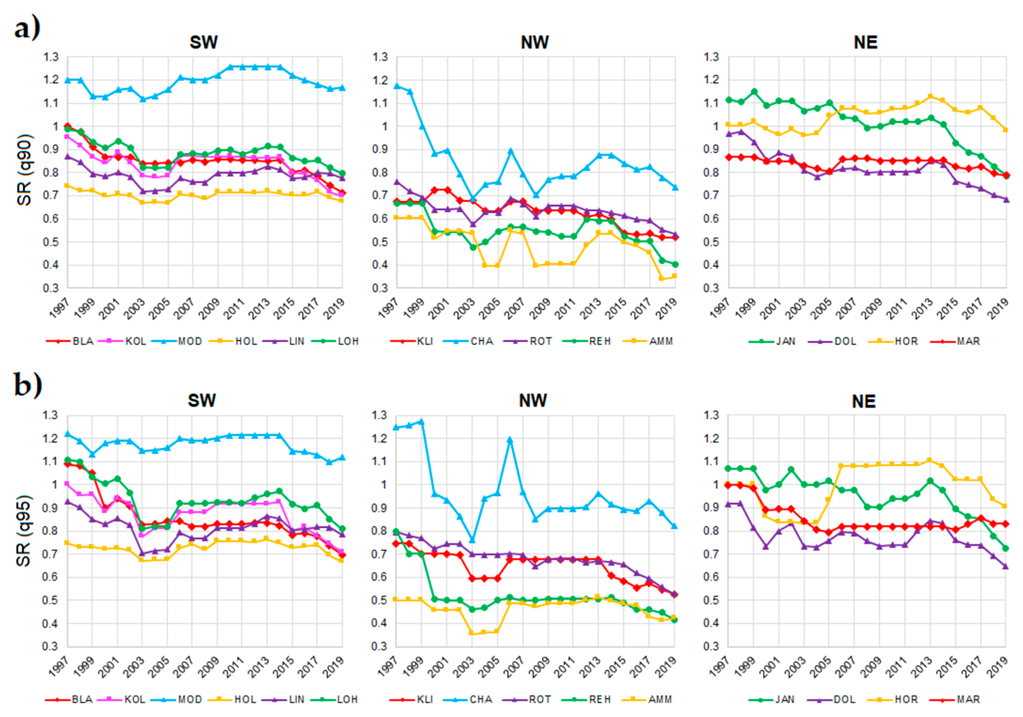
Long-term average values of the seasonality ratio (SR) provide a generalized information about the characteristics for the whole study period (

Table 3. Average values of the seasonality ratio (SR) for the 1968–2019 period.

	Southwestern Region (SW)						Northwestern Region (NW)					Northeastern Region (NE)
	BLA	KOL	MOD	HOL	LIN	LOH	KLI	CHA	ROT	REH	AMM	JAN	DOL	HOR	MAR
SR (q90)	0.85	0.85	1.20	0.70	0.85	0.91	0.59	0.94	0.62	0.50	0.45	0.97	0.83	1.01	0.82
SR (q95)	0.82	0.80	1.14	0.70	0.87	0.92	0.57	1.12	0.62	0.57	0.49	0.91	0.79	0.97	0.84

). The average SR for q90 and q95 ranged from 0.45 to 1.2 and 0.49 to 1.14, respectively. This indicates that the low-flow and drought regime in most of the catchments is closer to the summer type, but the seasonality is generally weak with values close to 1. The only catchment with SR > 1 for both q90 and q95 is MOD, suggesting that the winter low flows are slightly prevalent in this catchment.

The evolution of the SR was visualized by the 30-year moving averages. In most of the study catchments, the SR derived from the q90 series (Figure 2a) was generally decreasing in all regions with two exceptions (MOD in SW; HOR in NE), where the SR values remained relatively stable in the long-term horizon. The steepest decline was observed in most catchments of the NW region as well as in two catchments of the NE region (JAN, DOL). In most of the study catchments, the variability of SR calculated using the q95 series (Figure 2b) was distinctly greater, but the pattern of a decrease towards the summer low-flow regime was still apparent. Unlike the SR of the q90 series, all water gauges including MOD and HOR exhibited a decline even though the values varied significantly throughout the whole analyzed period. Assuming that the threshold between the winter and the summer low-flow regime was defined as SR = 1, eight out of fifteen catchments experienced a transition from the winter low-flow regime to the summer regime during the 1968–2019 period.

Long-term average values of the seasonality index (SI) components present the information about the characteristics for the complete 1968–2019 period (

Table 4. Average values of the seasonality index (SI) components for the 1968–2019 period.

	Southwestern Region (SW)						Northwestern Region (NW)					Northeastern Region (NE)
	BLA	KOL	MOD	HOL	LIN	LOH	KLI	CHA	ROT	REH	AMM	JAN	DOL	HOR	MAR
SI (Q90) Θ	4.41	4.37	5.89	4.05	4.82	4.90	4.31	4.87	4.51	4.19	4.26	4.72	4.52	5.01	4.74
SI (Q90) r	0.41	0.40	0.39	0.62	0.56	0.42	0.59	0.38	0.62	0.55	0.63	0.31	0.47	0.36	0.48
SI (Q90) D	256	254	342	235	280	284	250	283	262	244	248	274	262	291	275
SI (Q90) Date	13 September	11 September	8 December	23 August	7 October	11 October	7 September	10 October	19 September	1 September	5 September	1 October	19 September	18 October	2 October
SI (Q95) Θ	4.33	4.27	6.10	3.95	4.77	4.88	4.27	5.03	4.57	4.21	4.38	4.56	4.48	5.04	4.79
SI (Q95) r	0.51	0.59	0.45	0.69	0.59	0.40	0.70	0.38	0.69	0.52	0.71	0.47	0.58	0.45	0.60
SI (Q95) D	252	248	354	230	277	284	248	292	265	245	254	265	260	293	278
SI (Q95) Date	9 September	5 September	20 December	18 August	4 October	11 October	5 September	19 October	22 September	2 September	11 September	22 September	17 September	20 October	5 October

). In the catchments, the average occurrence of low flows (Q90) varied from 23 August to 8 December. The parameter r, which describes the concentration of the low-flow events during the year, ranged from 0.31 to 0.63.

The average occurrence of streamflow droughts (Q95) ranged from 18 August to 20 December, while the values of the parameter r varied between 0.38 and 0.71, meaning that the streamflow drought events (Q95) were generally slightly more concentrated in comparison with the low-flow events (Q90).

The 30-year SI moving averages for both Q90 and Q95 were plotted in polar graphs in order to visualize the joint evolution of the average low-flow/drought occurrence date along with the parameter r representing the level of concentration of such events during the year. In the catchments of the SW region (Figure 3), there is a common pattern of the increasing concentration of low flows and streamflow droughts. The most pronounced change of the concentration was observed in BLA and KOL, where the 30-year average values of the parameter r (Q95) rose from 0.25–0.35 to 0.7–0.8, whereas in the other catchments the increase was rather small. Changes were detected also in the average date of low-flow/drought occurrence. The most marked shift was observed in LOH, where the average day of Q95 occurrence moved by 74 days towards the beginning of the year, while in MOD, the shift was only six days. In all catchments of the SW region, the changes in the SI components were more eminent when using the Q95 quantile.

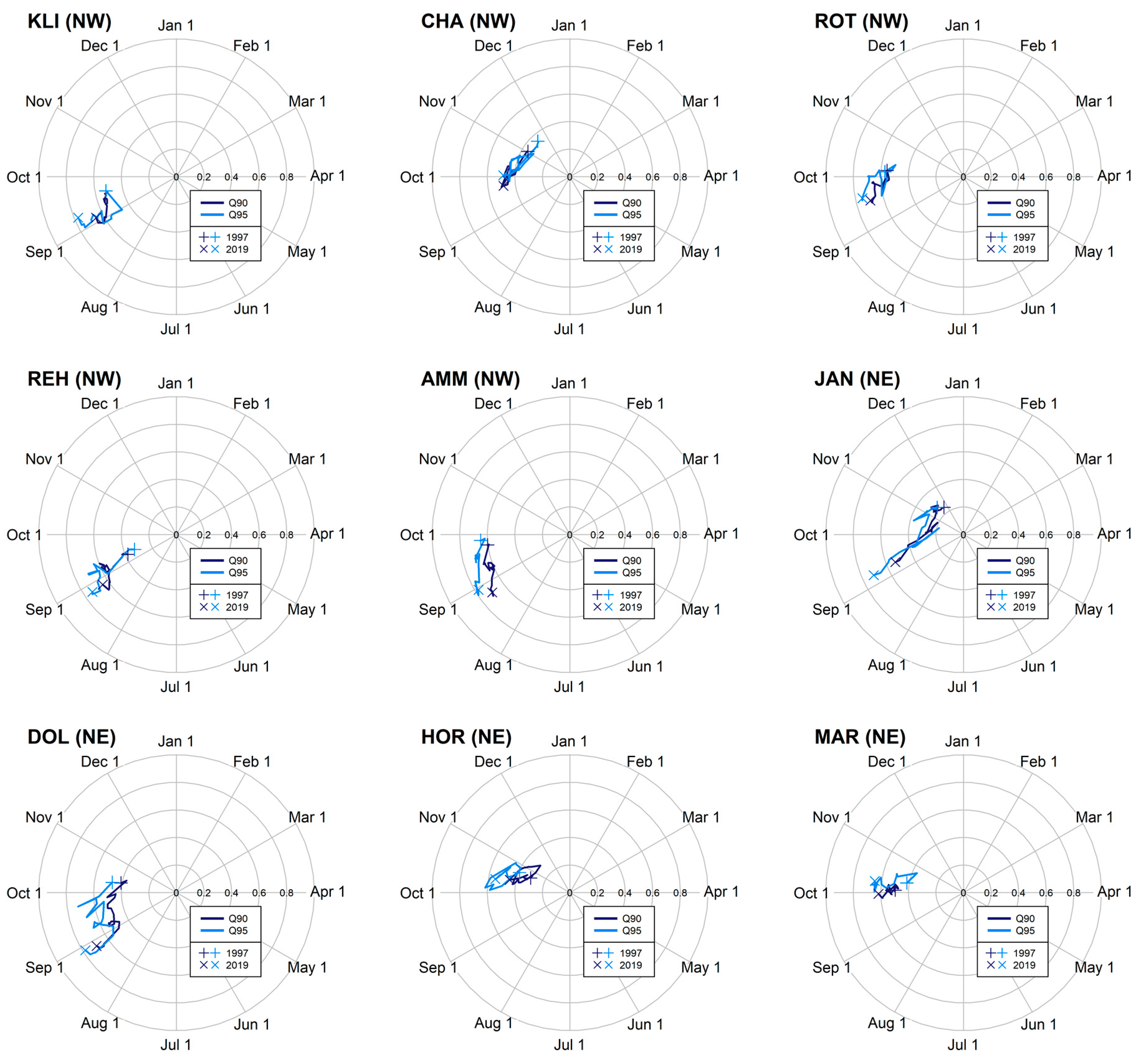
In the analyzed catchments of the NW and the NE region (Figure 4), the shifts in the values of SI components were more apparent for the Q95 quantile than for the Q90 quantile, similar to the situation in the SW region. The pattern of the increasing concentration of low flows and streamflow droughts was also present in all catchments of both regions. The most distinct shift in the average concentration of drought events occurrence was observed in REH (NW) and JAN (NE), where the values of the parameter r (Q95) rose by 0.41 and 0.44, respectively. In contrast, the smallest increase was detected in AMM (NW) and HOR (NE), where the parameter r rose by 0.13 and by 0.16, respectively.

The differences between catchments in terms of the average date of streamflow drought occurrence were rather distinct even within the individual regions. The most significant shift in the NW region was detected in CHA. The average day of Q95 occurrence moved in this catchment by 47 days towards the start of the year, whereas in KLI the shift was 11 days in the same direction. In the NE region, the most eminent shift was recorded in JAN (71 days), while in MAR, the shift was nearly negligible with only two days.

On average, for all study catchments, the increase of the parameter r (Q95) between the periods 1968–1997 and 1980–2019 was 0.24 and the average shift in streamflow drought occurrence was 28 days towards the start of the year. The catchments MOD, HOL and HOR were assessed as the most stable catchments regarding both seasonality parameters during the analyzed period.

3.2. Duration and Magnitude of Summer Streamflow Droughts Events

In general, the results of the seasonality analyses indicated that the streamflow drought events in the study catchments have an ongoing tendency to concentrate more in the warmer parts of the year. To quantify the real impact of the changing seasonal distribution of streamflow droughts, we examined the duration and deficit volumes of the actual streamflow drought events occurring within the summer season (1 April–30 November) in the catchments during the 1968–2019 period.

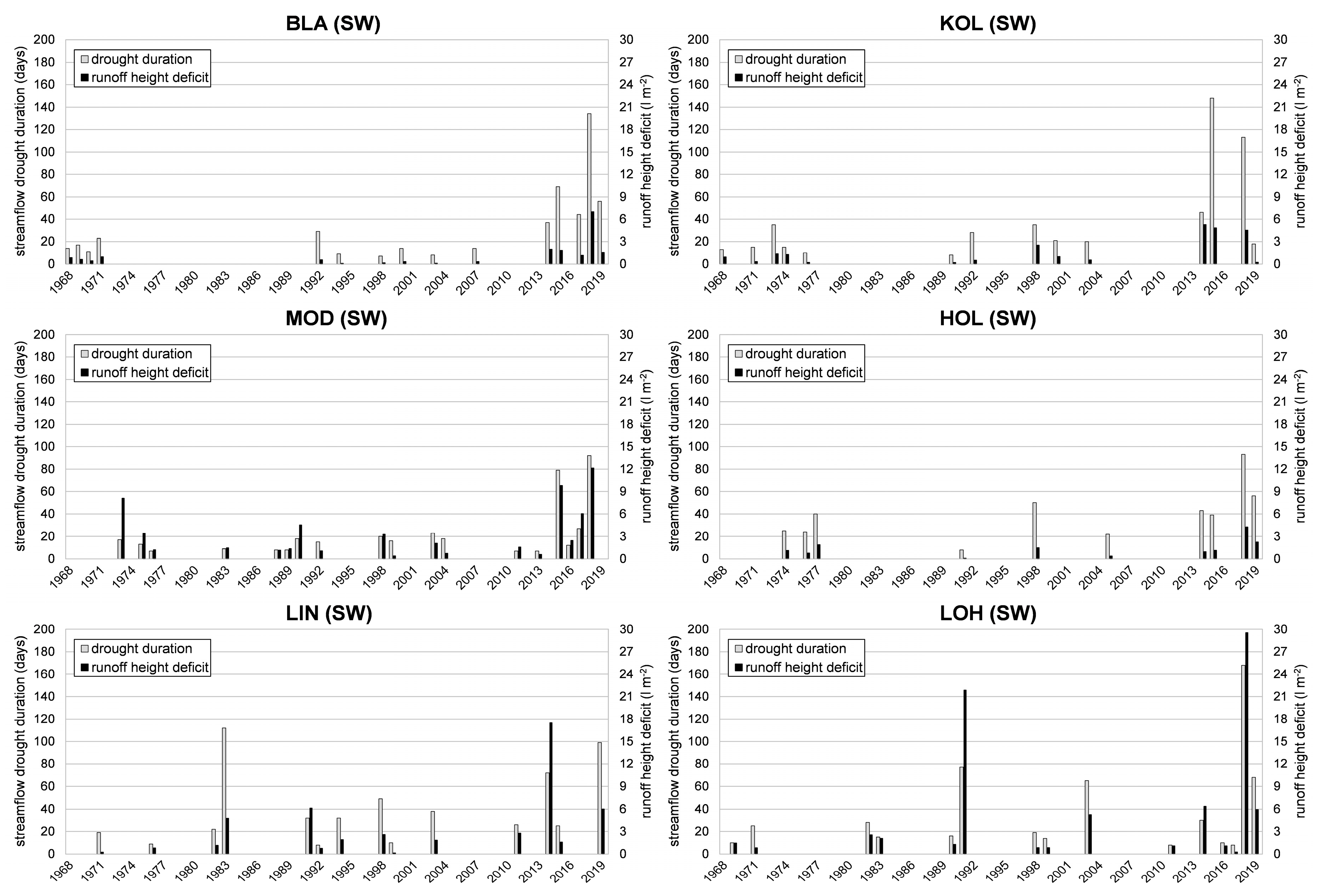
In four catchments within the SW region (BLA, MOD, HOL and LOH), the longest streamflow drought event was in 2018. In KOL and LIN, the longest drought events occurred in 2015 and in 1983, respectively. The other long-lasting streamflow droughts occurred in years 2014 (the third longest in KOL and LIN), 2015 (the second longest in BLA and MOD), and in 2019 (the second longest in HOL, LIN and the third longest in BLA, HOL and LOH). Regarding the magnitudes of streamflow droughts, the driest episodes occurred in 2018 (BLA, MOD and LOH), in 1991 (LOH), in 2015 (KOL and MOD) and in 2014 (LIN, KOL and LOH). In general, the drought episodes in BLA, KOL, MOD and LOH were longer and more severe by the end of the study period, whereas in LIN and LOH, the temporal distribution of the longest and the most intense droughts is more variable (Figure 5). The longest period of drought along with the greatest magnitude in the SW region was measured during the 2018 summer season in LOH, a total of 168 days and a 29.5 L m⁻² runoff height.

The longest streamflow drought event was recorded in four catchments of the NW region (KLI, ROT, REH and AMM) in 2018 (Figure 6). In the CHA catchment, the longest drought was recorded in the summer of 2003, which was also one of the driest years in KLI, ROT and AMM. The other long-lasting streamflow droughts occurred during the summer seasons of 2015 (the second longest in KLI), 2014 (KLI and CHA), 1975 in REH and 1976 in AMM. Regarding the magnitudes of streamflow droughts, the driest episodes occurred in 2014 and 2003 in the CHA catchment, in 2018 (KLI and ROT), in 1975 (REH) and in 1976 (AMM). Generally, the periods of streamflow drought in KLI, CHA and ROT were longer and more severe during the second half of the study period, while in REH and AMM the episodes were distributed more evenly across the 1968–2019 period. The longest drought in the NW region was recorded during the 2018 summer season in ROT (187 days). As for the drought magnitude, the greatest runoff height deficit was observed in CHA in the summer of 2014 (12.4 L m⁻²).

In the NE region, the longest streamflow drought was observed during the 2018 summer season in JAN, HOR and MAR (Figure 7). In the DOL catchment, the longest drought was recorded in the summer of 1983, which was also one of the driest years in JAN and HOR. The further remarkable streamflow droughts occurred in 1971 (DOL), 1976 (DOL), 1990 (JAN, DOL, HOR), 2003 (MAR), 2015 (JAN, HOR, MAR) and 2019 (JAN).

Regarding the magnitudes of streamflow droughts, the driest episodes occurred in 2018 (JAN, HOR, MAR), 1971 (DOL) and 1983 (HOR). In general, the streamflow drought events in JAN and HOR occurred relatively regularly with similar strength, whereas the droughts in MAR were more concentrated in the second half of the study period. The longest streamflow drought period within the NE region was recorded during the 2018 summer season in MAR (150 days) and the largest runoff height deficit was observed in JAN during the same year (16.5 L m⁻²).

3.3. Trends of Minimum Discharges

The trend analysis based on the series of mean summer minimum discharge (MSM-30; MSM-7) computed for the period from 1 April to 30 November was performed for all study catchments for the whole study period (

Table 5. The significance and direction of trends in the MSM-30 and MSM-7 time series (1968–2019) derived by the Mann–Kendall test. Trends are highlighted by three shades of orange (decrease) according to their statistical significance (no color for p ≥ 0.05; light for p < 0.05; medium for p < 0.01; dark for p < 0.001) along with the direction of Sen’s slope estimate (+ and −).

	Southwestern Region (SW)						Northwestern Region (NW)					Northeastern Region (NE)
	BLA	KOL	MOD	HOL	LIN	LOH	KLI	CHA	ROT	REH	AMM	JAN	DOL	HOR	MAR
MSM-30	−	−	−	−	−	−	−	–	−	−	−	−	+	−	−
MSM-7	−	−	−	−	−	−	−	–	−	−	−	−	+	−	−

) as well as for the 30-year moving windows.

The trend analysis of the MSM-30 series showed that a statistically significant (p < 0.05) decrease was detected only in five catchments (BLA, KOL, KLI, ROT and MAR). When testing the MSM-7 data series, the significant decline in MSM-7 was shown only in KLI, ROT and MAR. Moreover, there were not any significant trends in the SW region. The only catchment with long-term increasing tendency in both series was DOL; however, the trend was not significant.

The results of the trend analysis for the 30-year moving windows of MSM-30 (

Table 6. The significance and direction of trends derived for the 30-year moving windows of the MSM-30 series by the Mann–Kendall test. Trends are highlighted by three shades of orange (decrease) and blue (increase) according to their statistical significance (no color for p ≥ 0.05; light for p < 0.05; medium for p < 0.01; dark for p < 0.001) along with the direction of Sen’s slope estimate (+ and −).

	Southwestern Region (SW)						Northwestern Region (NW)					Northeastern Region (NE)
Period	BLA	KOL	MOD	HOL	LIN	LOH	KLI	CHA	ROT	REH	AMM	JAN	DOL	HOR	MAR
1968–1997	−	−	−	+	+	+	−	+	−	+	+	+	+	−	−
1969–1998	−	−	+	−	−	+	−	+	−	+	+	+	+	+	+
1970–1999	−	−	+	−	−	+	−	+	−	−	+	+	+	−	−
1971–2000	−	−	−	+	−	−	−	+	−	−	+	+	+	−	−
1972–2001	−	−	−	−	−	−	−	+	−	−	−	+	+	−	−
1973–2002	−	−	−	+	−	−	−	+	−	−	+	+	+	+	−
1974–2003	−	−	−	−	−	−	−	−	−	−	+	+	+	−	−
1975–2004	−	−	−	−	−	−	−	−	−	−	+	+	+	−	−
1976–2005	−	−	−	−	−	−	−	−	−	−	+	+	+	−	−
1977–2006	−	−	−	−	−	−	−	−	−	−	−	+	+	−	−
1978–2007	−	−	−	−	−	−	−	−	−	−	−	+	+	−	−
1979–2008	−	−	−	−	−	−	−	−	−	−	−	+	+	+	−
1980–2009	−	−	−	−	+	+	−	−	−	−	+	+	+	+	−
1981–2010	−	+	−	−	+	+	−	−	−	−	+	+	+	+	−
1982–2011	−	+	+	+	+	+	−	+	−	+	+	+	+	+	−
1983–2012	+	+	+	+	+	+	−	−	−	−	+	+	+	+	−
1984–2013	+	+	+	+	−	+	−	−	−	−	+	−	−	+	−
1985–2014	−	+	+	−	−	+	−	−	−	−	−	−	−	+	−
1986–2015	−	+	+	−	−	+	−	−	−	−	−	−	−	+	−
1987–2016	−	+	+	−	−	+	−	−	−	−	−	−	−	+	−
1988–2017	−	+	+	−	−	+	−	−	−	−	−	−	−	+	−
1989–2018	−	+	−	−	−	−	−	−	−	−	−	−	−	+	−
1990–2019	−	−	−	−	−	−	−	−	−	−	−	−	−	+	−

) showed a rather diverse pattern. The only two catchments with steadily decreasing tendency during the whole 1968–2019 period were ROT and KLI with the most significant decreases between 1974 and 2009 as well as in the intervals at the end of the study period.

In contrast, the values of MSM-30 were significantly increasing in DOL until 2005, making it the only catchment with significant increases during the whole study period. Moreover, DOL was also the only catchment which exhibited both significant increase and decrease, indicating an overall transition of the MSM-30 trend direction.

In general, statistically significant negative trends prevailed during the first half of the study period in the SW region, while the negative trends in the NW and NE region were more concentrated in the middle and at the end of the 1968–2019 period. The significant decrease during the 1977–2006 and 1978–2008 interval was detected in seven and six catchments across the study regions. The results also showed that there were six catchments across all study regions without a significant increasing or decreasing trend whatsoever (LIN, LOH, CHA, REH, AMM and HOR).

The results of the Mann–Kendall trend test for the MSM-7 series (

Table 7. The significance and direction of trends derived for the 30-year moving windows of the MSM-7 series by the Mann–Kendall test. Trends are highlighted by three shades of orange (decrease) and blue (increase) according to their statistical significance (no color for p ≥ 0.05; light for p < 0.05; medium for p < 0.01; dark for p < 0.001) along with the direction of Sen’s slope estimate (+ and −).

	Southwestern Region (SW)						Northwestern Region (NW)					Northeastern Region (NE)
Period	BLA	KOL	MOD	HOL	LIN	LOH	KLI	CHA	ROT	REH	AMM	JAN	DOL	HOR	MAR
1968–1997	+	−	−	+	−	+	−	+	−	+	+	+	+	−	−
1969–1998	+	−	−	+	−	+	−	+	−	+	+	+	+	−	−
1970–1999	−	−	−	+	−	−	−	+	−	−	+	+	+	−	−
1971–2000	−	−	−	+	−	−	−	+	−	−	+	+	+	−	−
1972–2001	−	−	−	+	−	−	−	+	−	−	+	+	+	−	−
1973–2002	−	−	−	+	−	−	−	+	−	−	+	+	+	−	−
1974–2003	−	−	−	−	−	−	−	+	−	−	+	+	+	−	−
1975–2004	−	−	−	−	−	−	−	+	−	−	+	+	+	−	−
1976–2005	−	−	−	−	−	−	−	−	−	−	+	+	+	−	−
1977–2006	−	−	−	−	−	−	−	−	−	−	+	+	+	−	−
1978–2007	−	−	−	−	−	−	−	+	−	−	+	+	+	−	−
1979–2008	−	−	−	−	−	−	−	−	−	−	+	+	+	+	−
1980–2009	−	−	−	−	−	−	−	−	−	−	+	+	+	+	−
1981–2010	−	−	+	−	+	+	−	−	−	−	+	+	+	+	−
1982–2011	−	+	+	+	+	+	−	+	−	+	+	+	+	+	−
1983–2012	−	+	+	−	+	+	−	+	−	+	+	+	+	+	−
1984–2013	−	+	+	−	+	+	−	−	−	+	+	+	−	+	−
1985–2014	−	+	+	−	−	+	−	−	−	+	+	−	−	+	−
1986–2015	−	+	+	−	−	+	−	−	−	−	−	−	−	+	−
1987–2016	−	+	+	−	−	+	−	−	−	−	−	−	−	+	−
1988–2017	−	+	+	−	−	+	−	−	−	+	−	−	−	+	−
1989–2018	−	−	−	−	−	+	−	−	−	−	−	−	−	+	−
1990–2019	−	−	−	−	−	−	−	−	−	−	−	−	−	+	−

) showed a relatively similar pattern to that of the MSM-30 series. Again, the only catchment observing the significant increasing trends was DOL. However, the significant increasing trends were detected only until 2004 and the transition to the significant decreasing trend took only 11 intervals instead of 13 detected in the MSM-30 series. The only catchments with decreasing MSM-7 during the whole 1968–2019 period were KLI, ROT and MAR with the most significant decreases between 1974 and 2010. In comparison with the trends in the MSM-30 series, the trend significance was slightly higher in KLI, ROT and MAR between 1977 and 2009. In ROT, JAN and DOL, the significant decreasing trends were detected also at the end of the analyzed period. In KLI, the significant declines were shown only in the first half of the study period. The results for MSM-7 showed no significant trends, either increasing or decreasing, in the same six catchments (LIN, LOH, CHA, REH, AMM and HOR).

The evaluation of trends in the 30-year steps of MSM-30 and MSM-7 provided a more synoptic image of the evolution and variability of the low-flow tendencies inside the 1968–2019 period. Furthermore, in the catchments of MOD, HOL, DOL, JAN and MAR, there were multiple 30-year intervals with a significant trend signal which showed the nonuniformity in the evolution of mean summer minimum flows as well as the most pronounced periods of change.

4. Discussion

The results of analyses of changes in the long-term variability and seasonality of low flows and streamflow droughts in 15 headwater, near-natural catchments of five different mountain ranges and highlands within the Central European region showed that not all of the established hypotheses can be sufficiently confirmed.

A shift in the seasonality ratio (SR) of low flows and streamflow droughts was apparent in most of the studied catchments. In two catchments with the average altitude above 1000 m.a.s.l. (MOD, HOR), the change was negligible suggesting that the ratio between summer and winter low flows remained almost the same at these sites throughout the 1968–2019 period. The relative stability of these two catchments during the study period is supported by the lowest average temperatures and the largest proportion of snow cover influencing the summer low flows [18,54], indicating that the warming has not significantly influenced the overall runoff balance of most montane catchments yet [12,27]. However, multiple studies suggest a further decrease in snow cover depth and snow water equivalent in montane areas of Central Europe, leading to a decrease in snowmelt contribution to summer runoff in the near future [27,31]. The most dynamic shifts were observed in the catchments with the mean elevation between 800 and 1000 m.a.s.l. A typical pattern for these catchments was a gradual decline in rates of winter low flows and streamflow droughts, which indicates that the consecutive warming in Central Europe affects these particular catchments the most. Catchments with the average elevation below 750 m.a.s.l. experienced generally just a minor decrease in values of the SR.

The changes in seasonality index (SI) differed among the study catchment as well. The behavior of the SI evolution during the analyzed period was in concordance with the evolution of SR. On average, the mean date of low flows has moved by approximately one month towards the start of the year. The most eminent shifts in the average low-flow date were detected in the catchments with the average altitude ~ 900 m.a.s.l. and with the prevailing hillslopes with S, SW and W direction across all of the study regions. Moreover, the low-flow and drought events exhibited an increasing tendency to occur in the same parts of the year within these catchments [4,10,31]. The two highest (MOD, HOR) and the two lowest (MAR, HOL) catchment showed minor changes in the average date of low-flow/drought occurrence during the 1968–2019 period.

The temporal distribution, duration and magnitude of the summer streamflow drought events were examined using the monthly (i.e., seasonally varying) threshold. Although the recent years, including 2018 and 2015 [14,20,21], have shown an increased occurrence of long-lasting severe droughts [8,11], this pattern may not be entirely valid for all of the study catchments. In some of them, the largest deficit volumes were observed during summer droughts in the 1970s and 1980s. The occurrence of summer streamflow droughts in Central Europe is also strongly dependent on the amount of snowpack in the previous winter [18,19]. Indeed, the recent long-lasting streamflow droughts indicate the potential increased proneness to such events in more than a half of the selected study catchments [25,26]. For a more representative assessment of droughts derived on the basis of the Q95 threshold and other necessary criteria, it would be better to use longer time series in order to make the resulting datasets less sparse [54,55,56]. However, such an approach would significantly affect the number of available catchments in this study because the areas of interest, mainly in the Ore Mountains (NW), have been gauged mostly since the 1960s.

Moreover, the effect of land cover changes in the catchments affected by forest disturbance might further enhance the effect of climate warming. Forest disturbances have an important role in snowmelt rates which might further affect the seasonal distribution of low flows [57]. Recent forest disturbances in the Ore Mountains [58] and the Bohemian Forest, caused predominantly by the infestation of bark beetle [28,30], should also indicate the streamflow feedback in the conditions of multiple changes of the environment in the near future [59,60,61]. The change points in long-term air temperature series detected in various studies between 1985 and 1995 [22,54,62] have been followed by increased frequency and intensity of low-flow events. This was further supported by our results, since the longest and most severe streamflow droughts occurred after 2000 in the major part of analyzed catchments. For most of the low-flow characteristics, there was no distinct difference between the regions, the similarities in low-flow regime were mostly found in the catchments with analogical properties across all regions. The initiation and persistence of streamflow droughts can be more dependent on local circulation of subsurface and surface water than on regional meteorological conditions [4]. Therefore, it seems to be crucial to further examine the reciprocal effects of the changing climate and the environmental characteristics of the near-natural catchments to clarify the mechanisms of runoff regime changes

5. Conclusions

The main objective of this paper was to evaluate the seasonality, magnitude and trends of selected low-flow and streamflow drought characteristics in five Central European montane and highland regions. We provided a comparison of different low-flow characteristics and seasonality indicators computed on the basis of daily streamflow data series in the 1968–2019 period in a set of fifteen near-natural headwater catchments located along the Czech–German and the Czech–Polish borders.

The outputs of this study, to some extent, confirmed the hypotheses that assumed the influence of the ongoing regional climate change on the ratio between summer and winter low flows and consequent changes in the seasonal distribution of low flows and streamflow droughts during the analyzed period.

We have shown a substantial reduction in the proportion of winter low-flow events expressed by the declining values of the seasonality ratio (SR) in the majority of study catchments. The regions with the highest average altitude appeared to be the most stable in terms of the balance between summer and winter low flows. Consequently, the results have proven the apparent shift in the low-flow and streamflow drought seasonality quantified by the components of the seasonality index (SI). In all study regions, the most pronounced seasonality shifts were detected in catchments oriented predominantly to the southwest and characterized by the mean altitude 800–1000 m.a.s.l. The hypothesis expecting a significant decrease in the mean summer minimum discharges in most of study catchment was not confirmed.

In this paper, only the hydrological characteristics were analyzed to provide an overview of the low flows and streamflow drought characteristics in fifteen headwater catchments in three regions of Central Europe. For a representative drought frequency analysis of low flows and droughts in the future, the catchments with the longest available streamflow data series should be chosen. Thereby, the following direction of research should also involve a detailed set of local climatic data in order to clarify the response of the low-flow regime in particular catchments.

References

- Valiya Veettil, A.; Mishra, A.K. Multiscale hydrological drought analysis: Role of climate, catchment and morphological variables and associated thresholds. J. Hydrol. 2020, 582. [Google Scholar] [CrossRef]
- Cervi, F.; Blöschl, G.; Corsini, A.; Borgatti, L.; Montanari, A. Perennial springs provide information to predict low flows in mountain basins. Hydrol. Sci. J. 2017, 62, 2469–2481. [Google Scholar] [CrossRef]
- Mishra, A.K.; Singh, V.P. A review of drought concepts. J. Hydrol. 2010, 391, 202–216. [Google Scholar] [CrossRef]
- Raczyński, K.; Dyer, J. Multi-annual and seasonal variability of low-flow river conditions in southeastern Poland. Hydrol. Sci. J. 2020, 00, 1–16. [Google Scholar] [CrossRef]
- Deb, P.; Kiem, A.S.; Willgoose, G. Mechanisms influencing non-stationarity in rainfall-runoff relationships in southeast Australia. J. Hydrol. 2019, 571, 749–764. [Google Scholar] [CrossRef]
- Van Loon, A.F. Hydrological drought explained. Wiley Interdiscip. Rev. Water 2015, 2, 359–392. [Google Scholar] [CrossRef]
- Zhong, R.; He, Y.; Chen, X. Responses of the hydrological regime to variations in meteorological factors under climate change of the Tibetan plateau. Atmos. Res. 2018, 214, 296–310. [Google Scholar] [CrossRef]
- Hänsel, S.; Ustrnul, Z.; Łupikasza, E.; Skalak, P. Assessing seasonal drought variations and trends over Central Europe. Adv. Water Resour. 2019, 127, 53–75. [Google Scholar] [CrossRef]
- Mozny, M.; Trnka, M.; Vlach, V.; Vizina, A.; Potopova, V.; Zahradnicek, P.; Stepanek, P.; Hajkova, L.; Staponites, L.; Zalud, Z. Past (1971–2018) and future (2021–2100) pan evaporation rates in the Czech Republic. J. Hydrol. 2020, 590, 125390. [Google Scholar] [CrossRef]
- Petek, M.; Kobold, M.; Šraj, M. Low-flow analysis of streamflows in Slovenia using R software and lfstat package. Acta Hydrotech. 2015, 27, 13–28. [Google Scholar]
- Trnka, M.; Balek, J.; Štepánek, P.; Zahradnícek, P.; Možný, M.; Eitzinger, J.; Žalud, Z.; Formayer, H.; Turna, M.; Nejedlík, P.; et al. Drought trends over part of Central Europe between 1961 and 2014. Clim. Res. 2016, 70, 143–160. [Google Scholar] [CrossRef] [Green Version]
- Langhammer, J.; Bernsteinová, J. Which Aspects of Hydrological Regime in Mid-Latitude Montane Basins Are Affected by Climate Change? Water 2020, 12, 2279. [Google Scholar] [CrossRef]
- Hanel, M.; Vizina, A.; Máca, P.; Pavlásek, J. A multi-model assessment of climate change impact on hydrological regime in the Czech Republic. J. Hydrol. Hydromech. 2012, 60, 152–161. [Google Scholar] [CrossRef] [Green Version]
- Hanel, M.; Rakovec, O.; Markonis, Y.; Máca, P.; Samaniego, L.; Kyselý, J.; Kumar, R. Revisiting the recent European droughts from a long-term perspective. Sci. Rep. 2018, 8, 1–11. [Google Scholar] [CrossRef]
- Vicente-Serrano, S.M.; Gouveia, C.; Camarero, J.J.; Beguería, S.; Trigo, R.; López-Moreno, J.I.; Azorín-Molina, C.; Pasho, E.; Lorenzo-Lacruz, J.; Revuelto, J.; et al. Response of vegetation to drought time-scales across global land biomes. Proc. Natl. Acad. Sci. USA 2013. [Google Scholar] [CrossRef] [Green Version]
- Orth, R.; Zscheischler, J.; Seneviratne, S.I. Record dry summer in 2015 challenges precipitation projections in Central Europe. Sci. Rep. 2016, 6, 1–8. [Google Scholar] [CrossRef]
- Blöschl, G.; Hall, J.; Viglione, A.; Perdigão, R.A.P.; Parajka, J.; Merz, B.; Lun, D.; Arheimer, B.; Aronica, G.T.; Bilibashi, A.; et al. Changing climate both increases and decreases European river floods. Nature 2019, 573, 108–111. [Google Scholar] [CrossRef]
- Jenicek, M.; Ledvinka, O. Importance of snowmelt contribution to seasonal runoff and summer low flows in Czechia. Hydrol. Earth Syst. Sci. Discuss. 2020, 1–23. [Google Scholar] [CrossRef] [Green Version]
- Blahušiaková, A.; Matoušková, M.; Jeníček, M.; Ledvinka, O.; Kliment, Z.; Podolinská, J.; Snopková, Z. Snow and climate trends and their impact on seasonal runoff and hydrological drought types in selected mountain catchments in Central Europe. Hydrol. Sci. J. 2020, 00, 1–14. [Google Scholar] [CrossRef]
- Laaha, G.; Gauster, T.; Tallaksen, L.M.; Vidal, J.-P.; Stahl, K.; Prudhomme, C.; Heudorfer, B.; Vlnas, R.; Ionita, M.; Van Lanen, H.A.J.; et al. The European 2015 drought from a hydrological perspective. Hydrol. Earth Syst. Sci. Discuss. 2016, 1–30. [Google Scholar] [CrossRef] [Green Version]
- Ionita, M.; Tallaksen, L.M.; Kingston, D.G.; Stagge, J.H.; Laaha, G.; Van Lanen, H.A.J.; Scholz, P.; Chelcea, S.M.; Haslinger, K. The European 2015 drought from a climatological perspective. Hydrol. Earth Syst. Sci. 2017, 21, 1397–1419. [Google Scholar] [CrossRef] [Green Version]
- Jehanzaib, M.; Shah, S.A.; Yoo, J.; Kim, T.W. Investigating the impacts of climate change and human activities on hydrological drought using non-stationary approaches. J. Hydrol. 2020, 588, 125052. [Google Scholar] [CrossRef]
- Brázdil, R.; Trnka, M.; Mikšovský, J.; Řezníčková, L.; Dobrovolný, P. Spring-summer droughts in the Czech Land in 1805-2012 and their forcings. Int. J. Climatol. 2015, 35, 1405–1421. [Google Scholar] [CrossRef]
- Forzieri, G.; Feyen, L.; Rojas, R.; Flörke, M.; Wimmer, F.; Bianchi, A. Ensemble projections of future streamflow droughts in Europe. Hydrol. Earth Syst. Sci. 2014, 18, 85–108. [Google Scholar] [CrossRef] [Green Version]
- Brunner, M.I.; Tallaksen, L.M. Proneness of European Catchments to Multiyear Streamflow Droughts. Water Resour. Res. 2019, 55, 8881–8894. [Google Scholar] [CrossRef] [Green Version]
- Stagge, J.H.; Kingston, D.G.; Tallaksen, L.M.; Hannah, D.M. Observed drought indices show increasing divergence across Europe. Sci. Rep. 2017, 7, 1–10. [Google Scholar] [CrossRef] [PubMed]
- Jenicek, M.; Seibert, J.; Staudinger, M. Modeling of Future Changes in Seasonal Snowpack and Impacts on Summer Low Flows in Alpine Catchments. Water Resour. Res. 2018, 54, 538–556. [Google Scholar] [CrossRef]
- Bernsteinová, J.; Bässler, C.; Zimmermann, L.; Langhammer, J.; Beudert, B. Changes in runoff in two neighbouring catchments in the Bohemian Forest related to climate and land cover changes. J. Hydrol. Hydromech. 2015, 63, 342–352. [Google Scholar] [CrossRef] [Green Version]
- Ledvinka, O. Evolution of low flows in Czechia revisited. Proc. Int. Assoc. Hydrol. Sci. 2015, 369, 87–95. [Google Scholar] [CrossRef]
- Langhammer, J.; Su, Y.; Bernsteinová, J. Runoff response to climate warming and forest disturbance in a mid-mountain basin. Water 2015, 7, 3320–3342. [Google Scholar] [CrossRef]
- Demirel, M.C.; Booij, M.J.; Hoekstra, A.Y. Impacts of climate change on the seasonality of low flows in 134 catchments in the River Rhine basin using an ensemble of bias-corrected regional climate simulations. Hydrol. Earth Syst. Sci. 2013, 17, 4241–4257. [Google Scholar] [CrossRef] [Green Version]
- Stahl, K.; Hisdal, H.; Hannaford, J.; Tallaksen, L.M.; Van Lanen, H.A.J.; Sauquet, E.; Demuth, S.; Fendekova, M.; Jódar, J. Streamflow trends in Europe: Evidence from a dataset of near-natural catchments. Hydrol. Earth Syst. Sci. 2010, 14, 2367–2382. [Google Scholar] [CrossRef] [Green Version]
- Kronenberg, R.; Franke, J.; Bernhofer, C.; Körner, P. Detection of potential areas of changing climatic conditions at a regional scale until 2100 for Saxony, Germany. Meteorol. Hydrol. Water Manag. 2015, 3, 17–26. [Google Scholar] [CrossRef]
- Franke, J.; Goldberg, V.; Eichelmann, U.; Freydank, E.; Bernhofer, C. Statistical analysis of regional climate trends in Saxony, Germany. Clim. Res. 2004, 27, 145–150. [Google Scholar] [CrossRef]
- Tolasz, R.; Míková, T.; Valeriánová, A.; Voženílek, V. Climate Atlas of Czechia, 1st ed.; Czech Hydrometeorological Institute, Palacký University Olomouc: Praha, Czech Republic, 2007; ISBN 978-80-86690-26-1. [Google Scholar]
- Langhammer, J.; Hartvich, F.; Mattas, D.; Rödlová, S.; Zbořil, A. The variability of surface water quality indicators in relation to watercourse typology, Czech Republic. Environ. Monit. Assess. 2012, 184, 3983–3999. [Google Scholar] [CrossRef]
- Czech Hydrometeorological Institute: Database of Surface Water Monitoring Network. Available online: http://portal.chmi.cz (accessed on 31 August 2020).
- Gewässerkundlicher Dienst Bayern: Runoff Bavaria, Bayerisches Landesamt für Umwelt. Available online: https://www.gkd.bayern.de/en (accessed on 2 September 2020).
- Sächsisches Landesamt für Umwelt, Landwirtschaft und Geologie: Hydrologische Daten. Available online: https://www.umwelt.sachsen.de/umwelt/infosysteme/lhwz/hydrologische-daten.html (accessed on 2 September 2020).
- Osborn, D.R.; Harvey, A.C. Forecasting, Structural Time Series Models and the Kalman Filter. Economica 1991, 58. [Google Scholar] [CrossRef]
- Golyandina, N.; Korobeynikov, A. Basic Singular Spectrum Analysis and forecasting with R. Comput. Stat. Data Anal. 2014, 71, 934–954. [Google Scholar] [CrossRef] [Green Version]
- Hyndman, R.J.; Khandakar, Y. Automatic time series forecasting: The forecast package for R. J. Stat. Softw. 2008, 27. [Google Scholar] [CrossRef] [Green Version]
- Laaha, G.; Blöschl, G. Seasonality indices for regionalizing low flows. Hydrol. Process. 2006, 20, 3851–3878. [Google Scholar] [CrossRef] [Green Version]
- Koffler, D.; Gauster, T.; Laaha, G. lfstat: Calculation of Low Flow Statistics for Daily Stream Flow Data. R Package Version 0.9.4. Available online: https://cran.r-project.org/package=lfstat (accessed on 12 September 2020).
- Young, A.R.; Round, C.E.; Gustard, A. Spatial and temporal variations in the occurrence of low flow events in the UK. Hydrol. Earth Syst. Sci. 2000, 4. [Google Scholar] [CrossRef] [Green Version]
- R Core Team R: A Language and Environment for Statistical Computing. Available online: https://www.r-project.org/ (accessed on 1 August 2020).
- Pohlert, T. trend: Non-Parametric Trend Tests and Change-Point Detection. R Package Version 1.1.4. Available online: https://cran.r-project.org/package=trend (accessed on 14 September 2020).
- Gustard, A.; Demuth, S. Manual on Low-flow Estimation and Prediction; World Meteorological Organisation: Geneva, Switzerland, 2008; Volume 50, ISBN 9789263110299. [Google Scholar]
- Fleig, A.K.; Tallaksen, L.M.; Hisdal, H.; Demuth, S. A global evaluation of streamflow drought characteristics. Hydrol. Earth Syst. Sci. 2006, 10, 535–552. [Google Scholar] [CrossRef] [Green Version]
- Tallaksen, L.M.; Madsen, H.; Clausen, B. On the definition and modelling of streamflow drought duration and deficit volume. Hydrol. Sci. J. 1997, 42, 15–33. [Google Scholar] [CrossRef]
- Hirsch, R.M.; Slack, J.R. A Nonparametric Trend Test for Seasonal Data With Serial Dependence. Water Resour. 1984, 20, 727–732. [Google Scholar] [CrossRef] [Green Version]
- Libiseller, C.; Grimvall, A. Performance of partial Mann-Kendall tests for trend detection in the presence of covariates. Environmetrics 2002, 13, 71–84. [Google Scholar] [CrossRef]
- Assani, A.A.; Landry, R.; Laurencelle, M. Comparison of interannual variability modes and trends of seasonal precipitation and streamflow in southern Quebec (Canada). River Res. Appl. 2012, 28, 1740–1752. [Google Scholar] [CrossRef]
- Kliment, Z.; Matoušková, M.; Ledvinka, O.; Královec, V. Trend analysis of rainfall-runoff regimes in selected headwater areas of the Czech Republic. J. Hydrol. Hydromech. 2011, 59, 36–50. [Google Scholar] [CrossRef] [Green Version]
- Spinoni, J.; Vogt, J.V.; Naumann, G.; Barbosa, P.; Dosio, A. Will drought events become more frequent and severe in Europe? Int. J. Climatol. 2018, 38, 1718–1736. [Google Scholar] [CrossRef] [Green Version]
- Khaliq, M.N.; Ouarda, T.B.M.J.; Gachon, P.; Sushama, L. Temporal evolution of low-flow regimes in Canadian rivers. Water Resour. Res. 2008, 44, 1–19. [Google Scholar] [CrossRef] [Green Version]
- Hotovy, O.; Jenicek, M. The impact of changing subcanopy radiation on snowmelt in a disturbed coniferous forest. Hydrol. Process. 2020, 1–17. [Google Scholar] [CrossRef]
- Kupková, L.; Potůčková, M.; Lhotáková, Z.; Albrechtová, J. Forest cover and disturbance changes, and their driving forces: A case study in the Ore Mountains, Czechia, heavily affected by anthropogenic acidic pollution in the second half of the 20th century. Environ. Res. Lett. 2018, 13. [Google Scholar] [CrossRef]
- Robinson, M.; Cognard-Plancq, A.L.; Cosandey, C.; David, J.; Durand, P.; Führer, H.W.; Hall, R.; Hendriques, M.O.; Marc, V.; McCarthy, R.; et al. Studies of the impact of forests on peak flows and baseflows: A European perspective. For. Ecol. Manag. 2003, 186, 85–97. [Google Scholar] [CrossRef]
- Sajikumar, N.; Remya, R.S. Impact of land cover and land use change on runoff characteristics. J. Environ. Manag. 2015, 161, 460–468. [Google Scholar] [CrossRef] [PubMed]
- Prudhomme, C.; Giuntoli, I.; Robinson, E.L.; Clark, D.B.; Arnell, N.W.; Dankers, R.; Fekete, B.M.; Franssen, W.; Gerten, D.; Gosling, S.N.; et al. Hydrological droughts in the 21st century, hotspots and uncertainties from a global multimodel ensemble experiment. Proc. Natl. Acad. Sci. USA 2014, 111, 3262–3267. [Google Scholar] [CrossRef] [PubMed] [Green Version]
- Alexander, L.V.; Tapper, N.; Zhang, X.; Fowler, H.J.; Tebaldi, C.; Lynch, A. Climate extremes: Progress and future directions. Int. J. Climatol. 2009, 29, 317–319. [Google Scholar] [CrossRef]
Figure 1.
Study catchments and their river gauging stations. Data: CHMI, GKD Bayern and LfULG.
Figure 2.
Evolution of the 30-year moving seasonality ratio (SR) at the water-gauging stations derived from (a) the q90 and (b) the q95 time series. Labels on the x axis represent the end year of every 30-year period (1997 represents the 1968–1997 period and so forth).
Figure 3.
Evolution of the SI (Date and r) using the 30-year moving average of Q90 (dark blue) and Q95 (light blue) in catchments within the SW region. Curves denote the evolution of SI in time, symbols represent the first (1968–1997) and the last (1990–2019) period of the 30-year SI average.
Figure 4.
Evolution of the SI (Date and r) using the 30-year moving average of Q90 (dark blue) and Q95 (light blue) in catchments of NW and NE regions. Curves denote the evolution of SI in time, symbols represent the first (1968–1997) and the last (1990–2019) period of 30-year moving average.
Figure 5.
Duration and runoff height deficits of streamflow drought events in the catchments of the SW region during the 1968–2019 period.
Figure 6.
Duration and runoff height deficits of streamflow drought events in the catchments of the NW region during the 1968–2019 period.
Figure 7.
Duration and runoff height deficits of streamflow drought events in the catchments of the NE region during the 1968–2019 period.