A Review of Tank Model and Its Applicability to Various Korean Catchment Conditions


1
Murray-Darling Basin Authority, Canberra 2601, Australia
2
H2R Inc., Ilsan, Goyang-si 10306, Korea
3
Department of Civil Engineering, Hongik University, Seoul 04066, Korea
*
Author to whom correspondence should be addressed.
Water 2020, 12(12), 3588; https://doi.org/10.3390/w12123588
Submission received: 25 November 2020
/
Revised: 17 December 2020
/
Accepted: 18 December 2020
/
Published: 21 December 2020
(This article belongs to the Section Hydrology)
Abstract
:This paper reviews a conceptual rainfall-runoff model called Tank which has been widely used over the last 20 years in Korea as a part of a water resource modelling framework for assessing and developing long-term water resource polices. In order to examine the uncertainty of model predictions and the sensitivity of model’s parameters, Monte Carlos and Markov chain-based approaches are applied to five catchments of various Korean geographical and climatic conditions where the catchment sizes are ranged from 83 to 4786 km2. In addition, three optimization algorithms—dynamically dimensioned search (DDS), robust parameter estimation (ROPE), and shuffled complex evolution (SCE)—are selected to test whether the model parameters can be optimized consistently within a narrower range than the uncertainty bounds. From the uncertainty analysis, it is found that there is limited success in refining the priori distributions of the model parameters, indicating there is a high degree of equifinality for some parameters or at least there are large numbers of parameter combinations leading to good solutions within model’s uncertainty bounds. Out of the three optimization algorithms, SCE meets the criteria of the consistency best. It is also found that there are still some parameters that even the SCE method struggles to refine the priori distributions. It means that their contribution to model results is minimal and can take a value within a reasonable range. It suggests that the model may be reconceptualized to be parsimonious and to rationalize some parameters without affecting model’s capacity to replicate historical flow characteristics. Cross-validation indicates that sensitive parameters to catchment characteristics can be transferred when geophysical similarity exists between two catchments. Regionalization can be further improved by using a regression or geophysical similarity-based approach to transfer model parameters to ungauged catchments. It may be beneficial to categorize the model parameters depending on the level of their sensitivities, and a different approach to each category may be applied to regionalize the calibrated parameters.
1. Introduction
A modeling framework has been an integral part of assessing and developing long-term water resource policies in Korea like any other country, and it is used to develop various scenarios for testing future water demands and water security to supply them [1]. Additionally, the modeling framework has been used to assist making policy decisions in water resource management so that numbers of services provided by water are maintained in a sustainable way for current and future users. The services in general include meeting traditional demands of domestic, industrial and irrigation uses; environmental and ecosystem requirements; and social and cultural needs.
With the given limitation of data availability, however, it is inevitable to use a rainfall-runoff model to complement historical data so that the inflows of the whole system can be estimated for a long period of time and used to assess various potential future scenarios. To this end, a conceptional rainfall runoff (CRR) model called Tank has been predominantly used in Korea over the last 20 years. The Tank model was initially proposed by Sugawara and Fuyuki [2] which consists of several tanks (or storages) serially connected with outlets from the tanks leading to surface and subsurface flows. Over the time, its conceptional representation has been expanded in attempts to capture hydrologic processes more accurately and completely.
In general, a CRR model needs to be calibrated against measured flow rates so that catchment dependent hydrologic processes are encapsulated in the model before its applications. Traditionally, the calibration is treated as a mathematical optimization problem where objective functions are defined as differences between measured and modeled flows and then a set of model parameters is searched in a direction of minimizing the objective functions. There are several studies of optimizing parameters of the Tank model. Yokoo, et al. [3] applied a Powell method [4] to find an optimal set of parameters of the model at 12 catchments in southern Japan which were then regionalized to ungauged catchments using their geographical characteristics. Chen, et al. [5] has compared two optimization algorithms introduced in [6]—the Multistart Powell and Shuffled Complex Evolution (SCE) methods. Kim, et al. [7] tested a multi-object genetic algorithm to optimize model parameters for various hydrologic flow regimes. There was a study focusing only on lower layered tanks of the model and their contributions to the recession part of hydrographs [8].
In light of an uncertainty estimation method introduced by Beven and Binley [9] called generalized likelihood uncertainty estimation (GLUE), there have been more focuses on Bayesian techniques and posteriori distributions of model parameters. More recently, the differential evolution adaptive Metropolis (DREAM) algorithm [10,11] is introduced to search parameter spaces more efficiently than the GLUE approach especially for applications where the parameters are correlated and high dimensional. A CRR model typically simulates complicated and complex hydrological processes within a catchment using one or more conceptual storages with a few parameters. It means that the model inherits some limitations in representing heterogenous characteristics of the catchment and simulating averaged behaviors. Even if field measurements such as rainfall intensities and flow rates are error free, the homogeneous assumption can bring errors into modeled flows, which are known as model structural errors [12]. Therefore, it is important to validate the model by applying the calibrated parameters to the period outside of the calibrated time span.
In developing the modeling framework, around 120 sub-catchments were identified across Korea and runoffs from them were calculated using the Tank model with four serially connected tanks and soil moisture stores at the top layer [1,5,13]. In general, the model parameters are calibrated for the limited catchments, and then its parameters are regionalized with catchment characteristics so that the model can be applied to the entire basin including ungauged catchments. There have been multiple attempts to establish regressed equations between the geographical characteristics and the model parameters [14,15].
This study aims to shed a light on the characteristics and uncertainty of the Tank model and to be a stepping-stone toward systematically rationalizing and regionalizing its parameters. The remainder of the paper is organized as follows. Section 2 introduces the Tank model and its key features. Section 3 discusses approaches to test the sensitivity and uncertainty of the model parameters. The three deterministic optimization techniques are then introduced. The model is calibrated at five catchments of various Korean geographical and climatic conditions where the catchment sizes are ranged from 83 to 4786 km2. In Section 4, the calibrated sets of parameters and their corresponding results are viewed in conjunction with the model uncertainty and the sensitivity of the model’s parameters. Model validation and cross-validation are also presented in this section. Key findings and future work are discussed in Section 5.
2. Tank Model
Since its first introduction by Sugawara and Fuyuki [2], many variations of the model have been proposed. Among them, a most well-known variant is with four layered tanks [3,5,16]. It consists of sets of linear tanks connected in series with the outlets on the side and bottom of the tanks. Water through the side outlets form surface and subsurface flows while groundwater saturation and seepage is represented by flows between the tanks. The version of the model used in this study also has four tanks (, , , ) but with additional capacity of groundwater soil moisture stores at the top tank (Figure 1, [13,16]). Kang, et al. [13] showed that the groundwater soil moisture improves baseflow behaviors significantly.
In essence, there are three types of parameters: (1) outlet coefficients () on the side and bottom of the tanks, 92) storage heights () to the outlets, and (3) the primary and secondary soil moisture stores ( and ) with their maximum capacity of and . Once the outlet coefficients are known, outflows () are calculated by
where denoting the four tanks and is the corresponding storage level. Note that the flows from the side outlets are named with subscript 1 or 2, and the seepage from an upper to lower tank is designated with subscript 0. storage in the top tank , has soil storage up to its maximum capacity of . If the soil storage is not fully saturated (i.e.,), water is supplied from the Tank by
where is the moisture exchange rate. Equation (2) indicates that is always positive and the primary soil moisture store is charged from the second layered Tank until . There are also soil moisture exhanges between the primary and secondary soil moisture stores as
where is the exchange rate between the two soil moisture stores. When is positive, moisture moves from the primary to secondary soil store, otherwise it moves from the secondary to primary store.
There are 16 parameters in total to be determined depending on initial storage levels, forcing functions such as precipitation, and catchment hydrologic characteristics. In this study, a warming up period of one year is used to remove impacts of the initial conditions.
3. Model Uncertainty and Optimization Algorithms
3.1. Model Uncertainty Estimation
For a hydrologic model whether it is conceptual or distributed, it possesses model errors [9,12]. A CRR model typically simulates complicated and complex hydrological processes within a catchment using one or more conceptual storages. It means that the model inevitably has limitations in representing heterogenous characteristics in the catchment and only averaged behaviors can be captured. The model errors caused by the homogeneous assumption is called model structural errors.
Beven and Binley [9] proposed the GLUE methodology to quantify the uncertainty of model predictions with a given model structure and errors in forcing and field observations. Compared to deterministic optimization techniques which normally lead to only one optimal parameter set, it results in a range of parameter sets which produces acceptable model results and is known as equifinality. Once multiple model simulations are obtained—often by using Monte Carlo sampling—the model results are grouped into behavioral and non-behavioral runs. The parameter sets from the behavioral runs can be accepted while the other parameter sets from the non-behavioral runs can be removed. In general, the performance of a parameter set is assessed by multiple likelihood functions. Therefore, successful applications of the GLUE framework are highly dependent on the choice of likelihood functions and more than one likelihood function would need to be selected in most cases [17]. Since its development, the GLUE approach has been widely accepted and used to test uncertainties of various hydrologic models [18,19] and other disciplines including water quality models [20,21], because of its flexibility and suitability for parallel computing in distributed systems.
However, a simple Monte Carlo sampling method can be computationally inefficient and may not be suitable to approximate complex and high-dimensional posterior distributions [22,23]. To improve the inefficiency, a Markov chain Monte Carlo (MCMC) sampling technique was introduced in the DREAM algorithm [10,11]. Some key advantages of the algorithm include operation of a randomized subspace sampling and outlier chain correction with multi-chains. Use of more than one chain with different starting points enables searching parameter spaces widely and exploring different trajectories of the posterior target distribution. It helps for applications with complex posterior distributions and correlated parameters [22].
In this study, a python package called SPOTYPY [24] is used to undertake an analysis of the uncertainty of the Tank model and the sensitivity of its parameters using a Monte Carlo based approach which is similar to what Houska, et al. [17] used for their study with the goodness-of-fit measure of three likelihood functions–coefficient of determination (), Bias (BIAS) and Nash-Sutcliffe efficiency (NSE). The DREAM algorithm is also tested, and its results are compared with the parameter sets developed from the GLUE approach.
3.2. Dynamically Dimensioned Search (DDS)
DSS is an algorithm introduced by Tolson and Shoemaker [25]. It efficiently scales the search to find good solutions as opposed to globally optimal ones within the maximum number of user-specified iterations. It is also parsimonious requiring only one parameter,, to tune the algorithm which makes this method easy to use. Therefore, it is potentially well suited for calibrating a conceptual hydrologic model with many parameters or a distributed watershed model which requires relatively large CPU time. The way it searches solutions is described below:
- Define a maximum number of iterations, .
- Populate an initial set of parameters, .
- Calculate hydrologic performance and allocate the best performing set to and .
- Generate a random number for each parameter space and select all parameter sets for perturbation when their random numbers are bigger than , where is the current iteration.
- Generate by perturbate for the selected parameters from Step 4 with a standard normal random variable of as , where , , is the parameter determining the perturbation range and is the total number of the parameter sets selected in Step 4.
- and , if .
- Go to Step 4 until the predefined maximum iteration is reached.
When the current iteration is increased, rapidly approaches to 0 and therefore the search dimension is getting smaller in Step 4. It means that the search space is global at the beginning of the iteration, but it gets more targeted toward the end of the iteration. The perturbation parameter is the recommended to be 0.2 in [25] and it is also used throughout this study.
Tolson and Shoemaker [25] compared performance of the DDS algorithm against the Shuffled Complex Evolution (SCE; [6,26]) in testing multiple optimization functions as well as calibrating parameters of hydrologic models. Their numerical tests showed that it was hard to distinguish the performances of the algorithms when numbers of model parameters were small (typically six or less). However, when they were applied to higher dimensional search problems the DDS approach was able to converge to a good set of parameters with fewer iterations.
As it is shown in the pseudo-code, however, it is a greedy type algorithm where a search direction is heuristically found based on known information and it never goes back to older iterations to update a better solution if found. It means that the solution at the end is potentially depending on where the search is started from, thereby not guaranteeing its global minimalization [27] and leading to the model locally optimized representation of hydrological behaviors.
3.3. Robust Parameter Estimation (ROPE)
ROPE is proposed by Bárdossy and Singh [28] and uses the depth function defined in [29] which was introduced as a graphical tool for visualizing data sets, but it is used to identify well performing parameter sets in this algorithm. The depth of a point measures how deep the point lies in the data set relative to its center. It means that the higher depth the closer to the central region of the data set. The algorithm is based on findings from [30] where geometrical structure of the best performing parameters in a 2-D searching space was studied, and a subsequent study extending it to multi-dimensional cases [28]. In their study, it was found that a set of parameters chosen based on the depth function was less sensitive to external disturbances such as potential measurement errors and performed well when it was transferred to a different time period. The depth function used in this algorithm is as follow:
- Select random data sets, .
- Measure their hydrological performances.
- Select best performing sets (10% of the initial sets), .
- Calculate the depths of every point in with respect to .
- Generate random parameter sets, such that the sets have higher depths with respect to .
- Replace with .
- Repeat Steps 2–6 until the performance from two samples are not significantly different or specified maximum iteration numbers are exceeded.
This algorithm implicitly implies that there is an iso-hypersurface of same depth. Model performances of parameter sets on the surface behave similarly and a set with a higher depth performs better. The use of the depth functions is recently received some attentions in various research areas [31,32,33] including a hydrologic study of flood frequency analysis [34].
3.4. Shuffled Complex Evolution (SCE)
The algorithm is developed for finding a set of globally optimized parameters of CRR models. It is also known as SCE-UA owing to developers’ affiliation, the University of Arizona (UA). Dual et al. [6] applied it to a model with up to six parameters and demonstrated its effectiveness to automatically calibrate the model. The algorithm involves the controlled random search, competitive evolution, and complex shuffling concepts as below.
- Generate samples using a uniform probability distribution from users defined bounds.
- Sort performances of the samples in increasing order.
- Divide the samples into partitions with points in each partition in a way that the nth partition contains every ranked point, where .
- Evolve each complex based on the competitive complex evolution (CCE, [35]).
- Combine the evolved points into a single sample then repeat Steps 2–5 until convergence criteria are satisfied.
As indicated by the cited numbers being more than 1300 (as of August 2020) of a subsequent paper on its optimal use [36], this algorithm has been very popular in calibrating and fining a set of good parameters [37] and found to be reliable for and capable of estimating optimum parameters for CRR models [38,39]. There have also been some cases of its applications to calibrate the Tank model [5,10].
4. Application
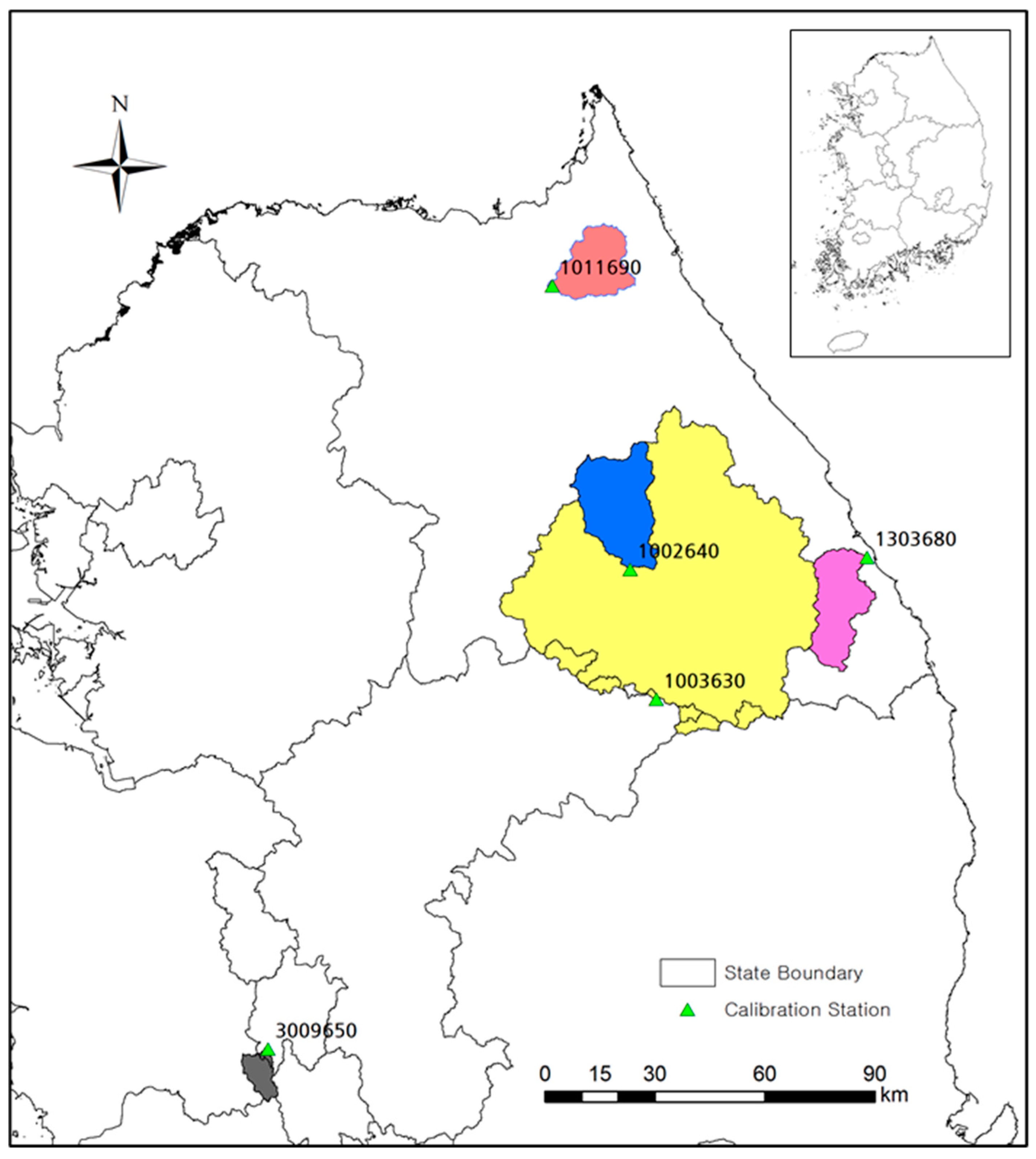
There are five flow stations selected for testing the model uncertainty and the performance of the three optimization algorithms in finding optimized parameter sets. The selected stations are located at upstream of major dams and not heavily affected by anthropogenic activities. As shown at Figure 2 and Table 1, the sites are selected to represent various catchment sizes from 83 to 4786 km2 where annual average rainfall of 1200~1600 mm per year is received on mountainous terrain leading to a high yield of runoffs.
For model calibration, a whole year is chosen to simulate daily discharges so that typical hydrological flow regimes can be included. It is found that year 2011 has a flow event of roughly 3 years return interval which is contributed by more than two rainfall events. In addition, there are also multiple small flash events and sufficient baseflows. Unless there are not enough quality flow data available, year 2011 is selected for calibration. Due to lack of consistent and quality data for the second and forth stations, however, years 2012 and 2018 are found to be more suitable, respectively. It should be noted that there is a lead time of one year allowed before measuring model performances in order to remove artificial sensitivity due to initial storage levels in the model.
4.1. Parameter Sensitivity and Uncertainty
Without knowing a priori distribution of the set of parameters, a uniform distribution is assumed to be reasonable where the parameter ranges are selected based on published results [6,8] with expert judgement. The three goodness-of-fit measures (R2, Bias and NSE) mentioned earlier are used to develop posterior distributions for the GLUE approach. R2 measures the deviation of modeled and observed data sets and is defined as:
where is the total number of measurements, is the observed value for the th measurement and is the corresponding data from the model. Similarly, and are the averages of the observed and modeled values. approaching to one indicates a strong linear relationship between the observed and modeled values. The bias function measures the differences between the two data sets as:
If the bias is positive the model is underpredicting, while it is negative when the model is overprediction. NSE is calculated as follows:
When the model perfectly matches the observed data (), then . If the nominator equals to the denominator, becomes zero. It indicates that the model has the same predictive capacity as using the average of the observed data. In addition to the three goodness-of-fit measures, mean absolute error (MAE) is often used as well. It is defined as:
In the DREAM approach, a likelihood function is used to evaluate a set of parameters. The likelihood function used in this study is calculated as:
where is the likelihood function which is also known as the Gaussian likelihood with measurement error integrated out [20].
For the GLUE approach, 106 parameter sets are created randomly in a uniform distribution. Simulated results using the initial parameter sets are compared with observed discharges by using the three performance measures. All parameter sets resulting in the performance measures within acceptable ranges are kept for developing posterior distribution. The acceptable ranges in this study are defined as , and .
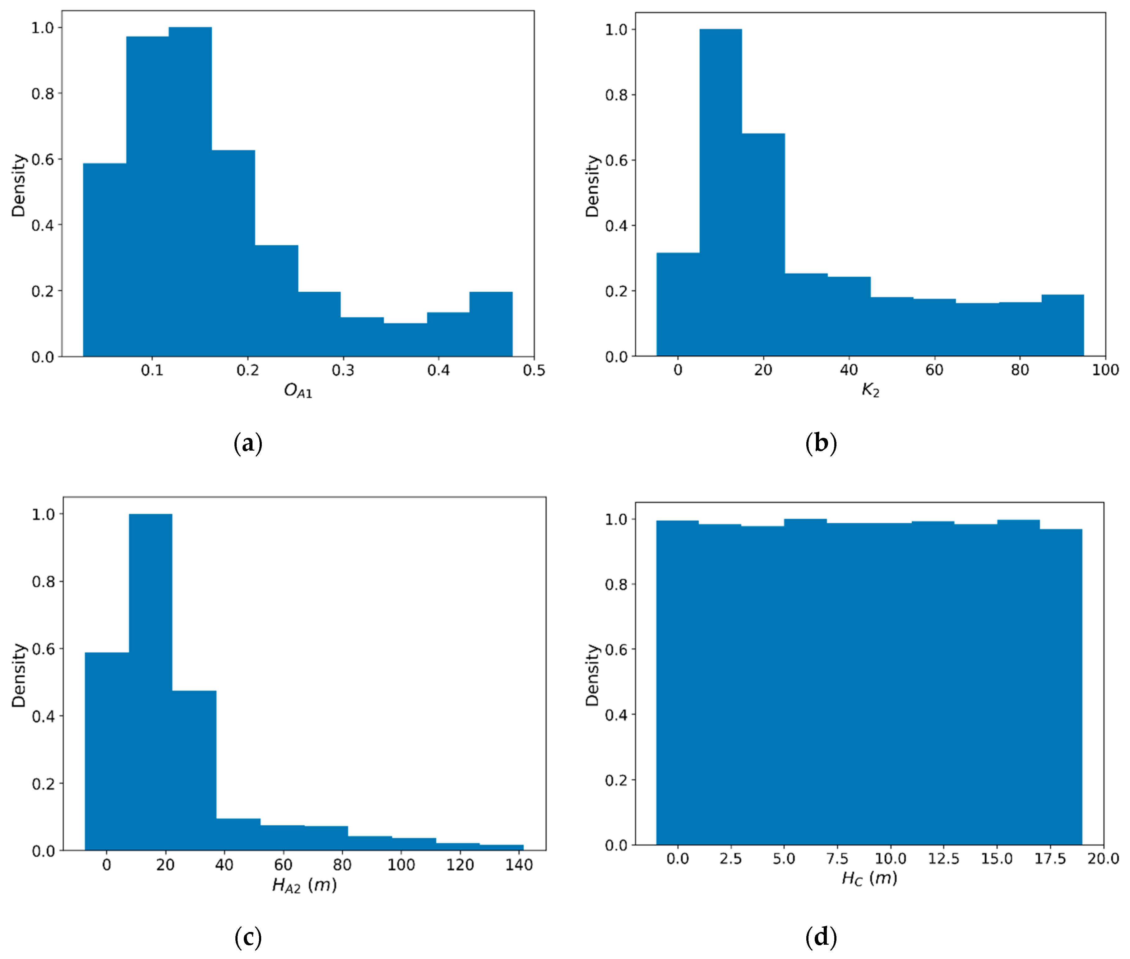
Figure 3 and Figure 4 present the posterior distributions and ranges of selected parameters for the GLUE and DREAM approaches at Station 1002640. To illustrate parameter uncertainty, there are three more sensitive and one less sensitive parameters presented. For the three sensitive parameters, the GLUE approach shows some refinement from their initial uniform distributions while the DREAM approach improves them significantly. As shown in Figure 3a and Figure 4a, the most a-posteriori value for the constraint of the lower outlet at Tank A ( is found to be quite different depending on an approach used. A similar behavior is observed for the storage level to the upper outlet at Tank A (, Figure 3c and Figure 4c). This is most likely due to interactions between parameters where a higher value of one parameter can be counterbalanced by a lower value of other parameters. As explained earlier, it demonstrates that the DREAM algorithm can outperform the GLUE in shaping parameter spaces and their distributions for cases with complex posterior distributions and correlated parameters. However, there is no significant differences between the approaches adopted for the insensitive parameter (Figure 3d and Figure 4d). It is found that the parameters associated with the top two tanks are responsive as they produce most of direct surface runoffs. The bottom two tanks contribute subsurface and base flows, and their linked parameters are generally less sensitive indicating a high degree of equifinality.
Figure 5 shows that simulated discharges from the tank model and the parameter uncertainty derived from both approaches. It indicates that most of observed discharges are within the uncertainty range. In general, the model overpredicts pulse like small events and underpredicts peaks of high flow events especially when they are compounded by multiple rainfall events. These behaviors are more pronounced when the GLUE approach is used as it increases the parameter uncertainty.
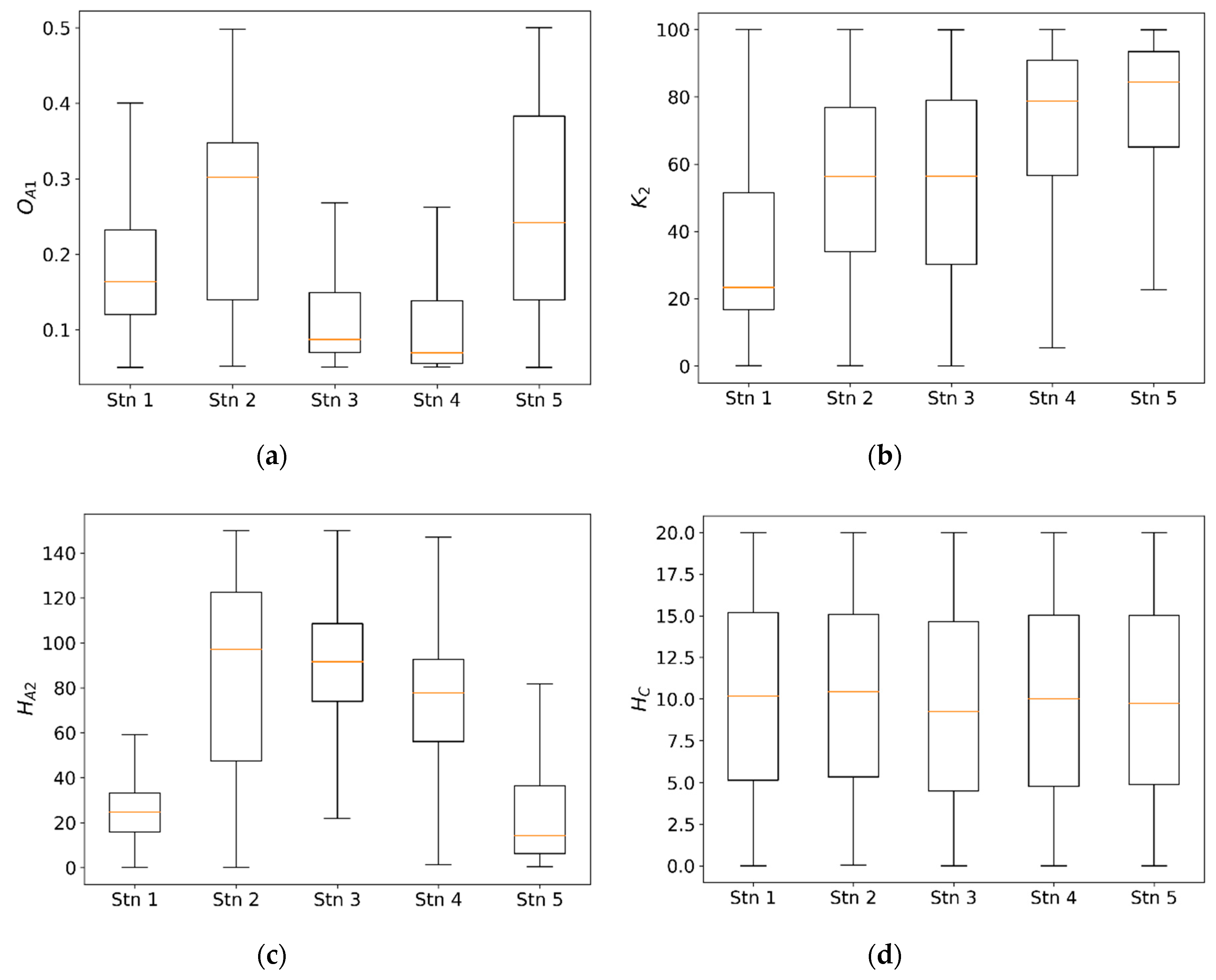
Similar to Figure 3 and Figure 4, the posteriori distributions of the four parameters derived from the two approaches are presented at Figure 6 and Figure 7 where the key findings observed from Station 1,002,640 (Figure 3 and Figure 4) are repeated from the other stations. These figures repeatedly show the superiority of the DREAM approach in refining the posterior distributions across the five calibration stations. However, both approaches are incapable of refining the parameters associated with the lower two tanks as indicated in Figure 6d and Figure 7d.
In the next section, the three traditional optimization techniques introduced earlier are tested for their capacity to find a set of parameters consistently across the calibration stations. It is also reviewed whether the optimization techniques can refine the insensitive parameters that are identified during the GLUE and DREAM analysis.
4.2. Comparison of the Optimization Algorithms
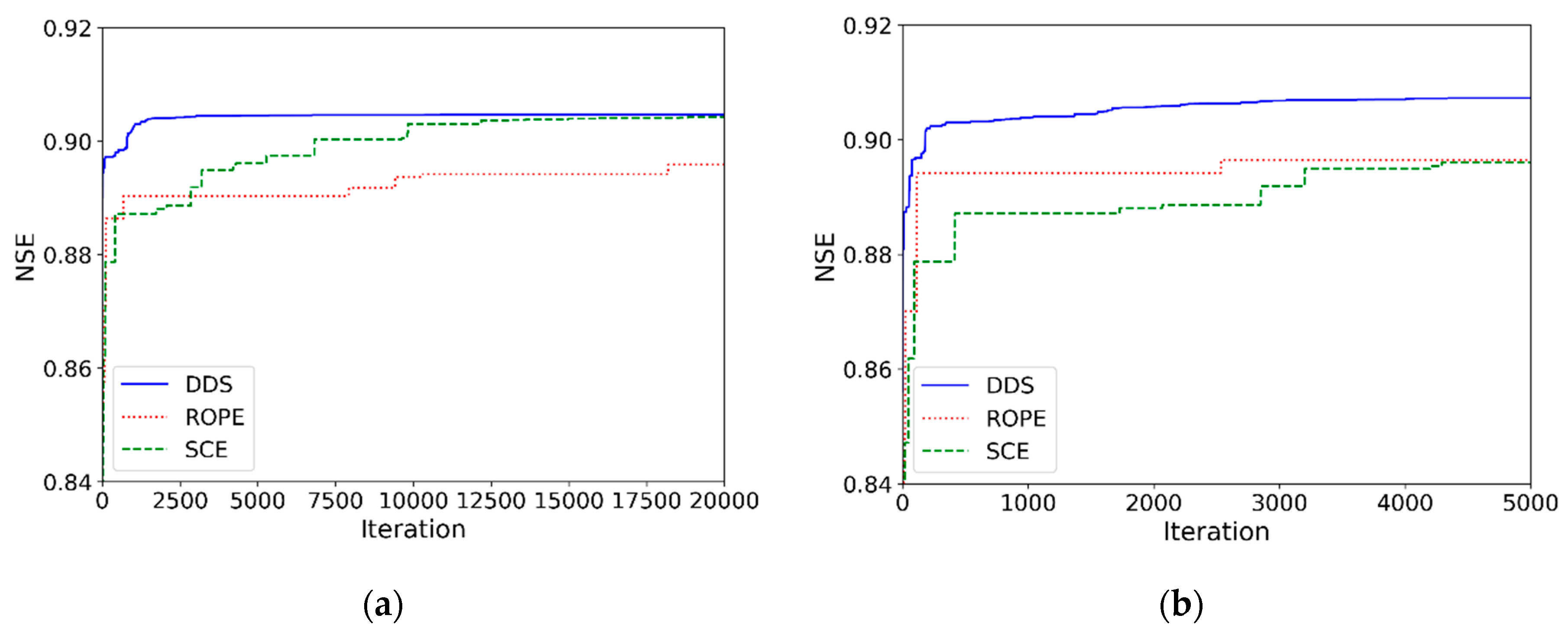
The three optimization algorithms are tested for the stations listed at Table 1. Similar to the GLUE and DREAM approaches, calibrations are conducted for the whole year identified in the Table 1. A lead time of one year is added before measuring model performance so that the effects of initial conditions are minimized. Firstly, the convergency rate of the algorithms is examined. There are two test cases by setting different numbers of maximum iterations—5000 and 20,000. Figure 8 shows that the three algorithms perform well and converge to a reasonable level but with slightly different accuracies. ROPE tends to search solution spaces well but not deep enough thereby showing that the objective function is maximized to a slightly lower degree than the other algorithms. As demonstrated in [22], DDS converges quicker than the other two algorithms. When a number of iterations are sufficiently large enough, SCE can equally perform well compared to the DDS algorithm (Figure 8a). The figure shows that decreasing iterations from 20,000 to 5000 does not hamper the capacity to minimize the objective function when DDS is used (Figure 8b).
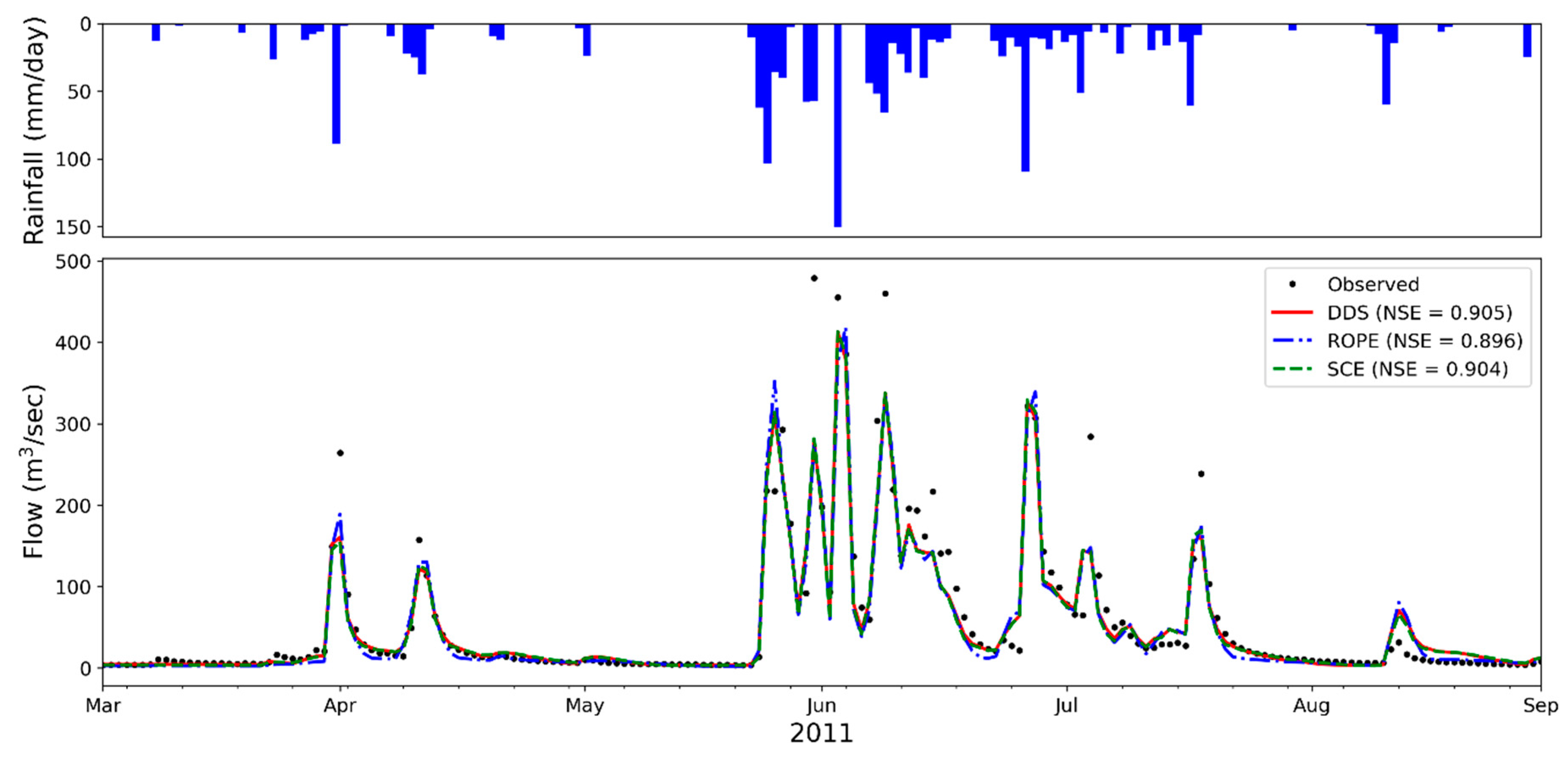
Table 2 summarizes the performance of the three optimization algorithms with various performance measures. Overall, it does not show any significant superiority among the three algorithms. As an indication, results at Station 1002640 are presented in Figure 9 showing the calibrated flows using the three optimization algorithms. This figure shows that all three algorithms perform equally well with no significant difference in NSE values. For Station 1003630, although NSE and R2 values indicate that the algorithms can sufficiently match historical data, it seems that modeled results are biased toward to underprediction given BIAS being negative and MAE higher than the other stations.
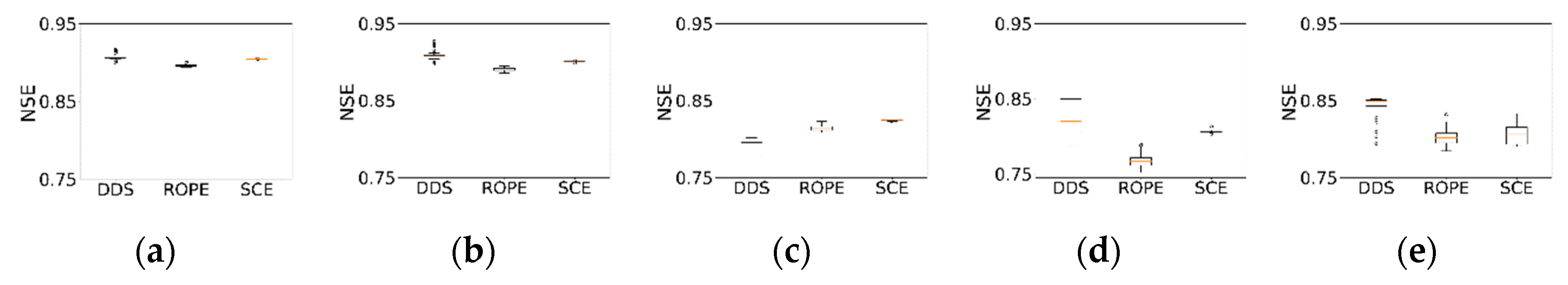
Based on Figure 8 and Figure 9 and Table 2, the DDS algorithm seems a reasonable choice being able to find a good set of parameters within a small number of iterations. As explained earlier, however, it is a greedy type algorithm where a globally optimized solution is not guaranteed. It means that the convergence of the set of parameters is highly dependent to an initial set. ROPE also possesses a similar behavior when the depth function is applied. To test the dependency to initial parameter sets, there are 100 calibration trials developed with different initial sets of randomly chosen parameters. Each trial runs 20,000 iterations for all algorithms. Figure 10 presents the goodness-of-fit measured by NSE and its distribution over the 100 trials. It shows that the DDS scheme has potential to outperform the other algorithms demonstrated by higher NSE values at most calibration stations. As explained earlier, however, final solutions using the DDS and ROPE methods are dependent to their starting initial sets of parameters with slightly stronger dependency observed with DDS. For most cases, the SCE method shows lesser tendency than the others and is able to repeatedly find solutions within much smaller ranges regardless their starting parameter sets. The only exception is Station 3,009,650 where the size of the catchment is the smallest out of the examined stations.
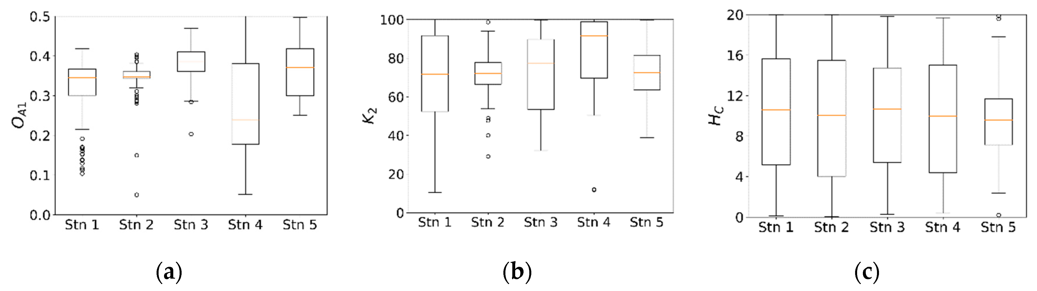
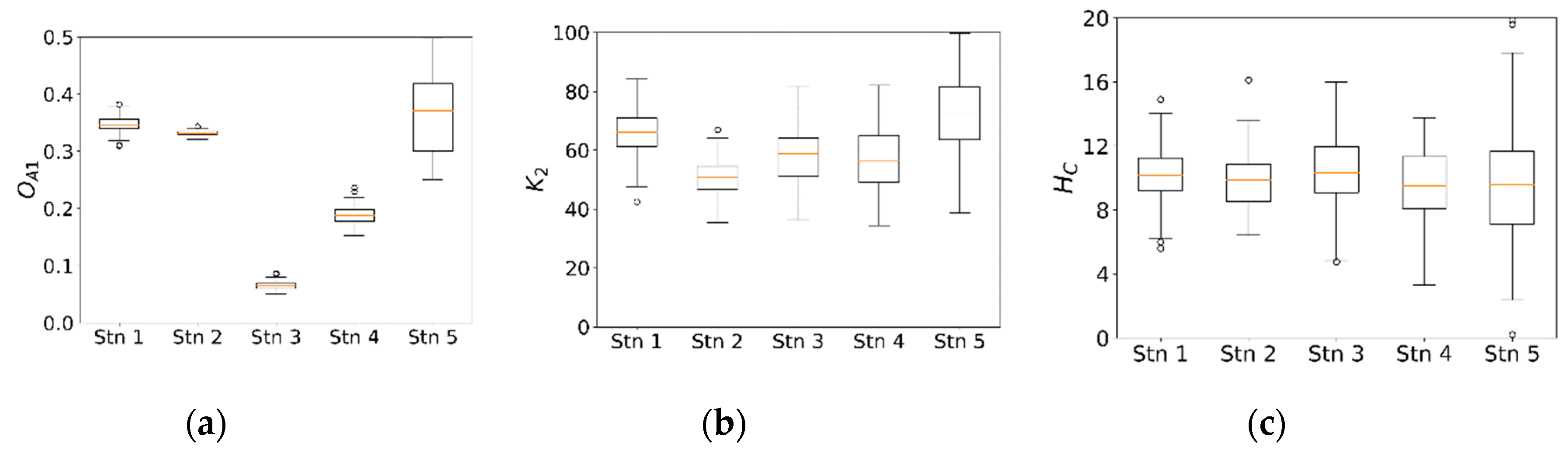
In lieu of formally estimating parameter uncertainty and its likelihood distribution, the results developed from the 100 trials are used as a surrogate to review whether an optimization algorithm can narrow the uncertainty bounds of model parameters. Arsenault and Brissette [40] used a similar approach to study the effects of parameter equifinality when a hydrologic model is applied for predicting streamflow in ungauged catchments. Similar to Figure 6 and Figure 7, two sensitive parameters ( and ) and one insensitive parameter () are selected and their distributions are presented in Figure 11, Figure 12 and Figure 13. These figures show that the optimization techniques especially the SCE algorithm can reduce parameter uncertainty even further from the refinements achieved by the GLUE and DREAM approaches. However, there is still limited success in scoping the ranges of the insensitive parameter. Figure 11c, Figure 12c and Figure 13c) show that the final distribution of closely resembles to its initial uniform distribution, which is ranged from 0 to 20 m. It indicates that the selection of this parameter does not affect model results greatly and a value may be chosen within a reasonable range without affecting model performance.
As mentioned by Arsenault and Brissette [40], the equifinality can be an issue for regionalization when a regression or geophysical similarity-based approach is used. With a high level of equifinality, model parameters of two similar catchments could be uncorrelated and some model parameters may not be strongly correlated to geographical characteristics. It is also possible that one catchment characteristic can be mapped to a range of values for one model parameter.
4.3. Validation
The calibrated parameter sets from the 100 simulations for each station are evaluated by applying them to the different periods identified at Table 1. The model validation is performed using the 100 sets of parameters found from Section 4.2. Table 3 summarizes the outcomes from the validation with the model performance measured by NSE values in the form of the median and variation from the 100 validation simulations for each station where the variation is expressed as the difference between the 5th and 95th percentile NSE measures. The validation results can be compared against the calibration performance of Table 2 and Figure 10. It indicates that the model performance is slightly reduced when the calibrated parameters are applied to the different periods, but the results are still within an acceptable range demonstrating their applicability. In general, the validation outcomes mimic the calibration behavior. For example, Stations 1,011,690 and 1,303,680 show lower NSE values than the others, and the DDS and ROPE algorithms produce wider variations in the NSE values.
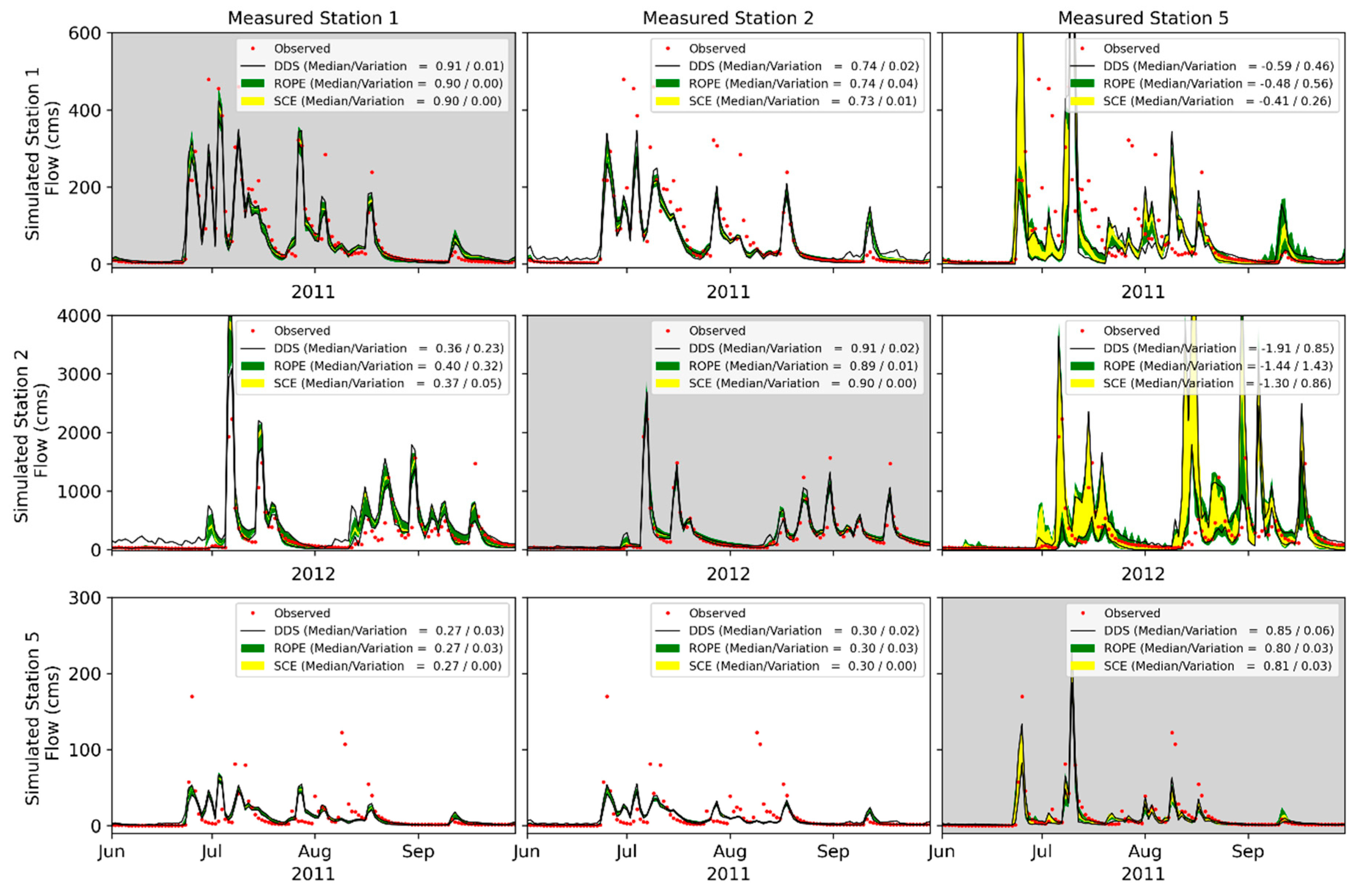
Further to the model validation, a cross-validation is undertaken by selecting calibrated parameters from one station and applying them to other stations to evaluate the applicability of calibrated parameters to ungauged catchments. For the process, three sites (Stations 1002640, 1003630 and 300650) are chosen. Stations 1002640 and 1003630 are closely located together (Figure 2) thereby sharing similar geographic and rainfall characteristics (Table 1). However, Station 3009650 is remotely located from the two sites with the smallest catchment size out of the five sites tested in this study. Key outcomes from the cross-validation are visualized in Figure 14. In general, calibrated parameters work well between Stations 1002640 and 1003630, indicating a high level of transferability. The comparison shows catchment area dependent model behavior. Applying calibration parameters from a smaller catchment (Station 1002640) to a bigger catchment (Station 1003630) makes the model overpredict. The opposite application leads to underprediction of discharges. This behavior is much prominent for the application with the smaller catchment (Station 1003630). Model performance drop significantly when the parameters from the first two sites applied to Station 3009650. The parameters calibrated at the small site reflect the quick response, and applying them to the other two bigger sites leads to highly overpredicted modeled results. On the other hand, when the parameters from the first two sites applied to Station 3009650, modeled results are underpredicted. It suggests that regionalization should factor in geophysical similarity and it is potentially improved further if some relationships between model parameters and catchment characteristics are developed and applied.
5. Conclusions
This study has reviewed the Tank model which has been prevalently used as a part of a water resource modeling framework for more than the last 20 years in Korea to develop long-term management policies of water related issues. This study gives a well-deserved spotlight on the model given its general acceptance within the hydrologic society in Korea without having enough focus on its applicability across various Korean conditions.
The model has examined for the selected five typical catchments. Firstly, a Monte Carlos based GLUE analysis is performed to quantify the uncertainty of model predictions with a given model structure and errors in forcing and field observations. It is found that there are little or no significant changes between the priori and posterior distributions for some parameters, indicating there is a high degree of equifinality or at least there are large numbers of parameter combinations leading to good solutions within model’s uncertainty bounds. It has shown that the DREAM approach, using more than one chains with different starting points searching parameter spaces widely and exploring different trajectories of the posterior target distribution, performs better in shaping parameter spaces and their distributions for cases with complex posterior distributions and correlated parameters.
To test this, three algorithms are selected including the DDS, ROPE, and SCE algorithms. Then their capacity of finding a set of optimized parameters consistently independent to their initial starting conditions is examined. All optimization algorithms perform well to refine the ranges of most parameters although the SCE method meets the criteria of the consistency best. However, it is also found that even the optimization algorithms struggle to refine the priori distributions of some parameters. It means that there are some parameters insensitive to catchments applied and can take a value within a range without compromising modeled solutions. Alternatively, the model can be reconceptualized to be parsimonious by reducing number of layers in the model for example and some parameters could be combined if model’s capacity to replicate historical flow characteristics is not affected.
The application of calibrated parameters to different periods indicates that the model is applicable to other runoff simulations within acceptable accuracy even though slightly wider variation in model results is observed in the DDS and ROPE algorithms. The cross-validation of applying calibrated parameters at one site to others shows some promising outcomes when two catchments are located closely each other. It is also found that the calibration parameters can lead to unrealistic results when they are transferred to a catchment that does not share geophysical characteristics. It suggests that regionalization can be further improved if relationships is established between model parameters and key characteristics of ungauged catchments.
Even though the SCE algorithms can optimize parameters within a smaller uncertainty band, it is still problematic to develop regression equations or geophysical similarity criteria. This is because one catchment characteristic can be mapped to a range of values for one model parameter. We plan to further extend this study to establish a systematic approach of regionalizing model parameters with consideration of their uncertainty. The model parameters may be categorized by whether they are strongly dependent to the model or site characteristics. Different regionalization approaches may be useful to the different categories. Additionally, machine learning techniques may be of great use to compliment the traditional regression approaches to develop relationships between the model parameters and catchment characteristics.
Author Contributions
Conceptualization, J.W.L. and S.D.C.; methodology, J.W.L. and S.O.L.; software, J.W.L.; validation, J.W.L., S.D.C. and S.O.L.; formal analysis, J.W.L., S.D.C. and S.O.L.; investigation, J.W.L., S.D.C. and S.O.L.; resources, S.O.L.; data curation, J.W.L.; writing—original draft preparation, J.W.L.; writing—review and editing, J.W.L., S.D.C. and S.O.L.; visualization, J.W.L.; supervision, S.O.L.; project administration, S.O.L.; funding acquisition, S.O.L. All authors have read and agreed to the published version of the manuscript.
Funding
This research received no external funding.
Acknowledgments
Lee Jong Wook was supported by Brain Pool Program through the National Research Foundation of Korea (NRF) funded by the Ministry of Science and ICT (Grant No.: 2019H1D3A2A01102253) and Lee Seung Oh was supported by the National Research Foundation of Korea (NRF) grant funded by the Korea government (MSIT) (NRF-2017R1A2B2011990)
Conflicts of Interest
The author declare no conflict of interest.
References
- MLIT. Long Term Water Resource Plan (2001-2020), 3rd ed.; Ministry of Land, Infrastructure and Transport (MLIT); Government of South Korea: Seoul, Korea, 2016. [Google Scholar]
- Sugawara, M.; Fuyuki, M. A Method of Revision of River Discharge by Means of a Rainfall Model. In A Collection of Research Papers about Forecasting Hydrologic Variables; The Geosphere Research Institute of Saitama University: Saitama, Japan, 1956; pp. 14–18. [Google Scholar]
- Yokoo, Y.; Kazama, S.; Sawamoto, M.; Nishimura, H. Regionalization of lumped water balance model parameters based on multiple regression. J. Hydrol. 2001, 246, 209–222. [Google Scholar] [CrossRef]
- Powell, M.J.D. An efficient method for finding the minimum of a function of several variables without calculating derivatives. Comput. J. 1964, 7, 155–162. [Google Scholar]
- Chen, R.-S.; Pi, L.-C.; Hsieh, C.-C. Application of parameter optimization method for calibrating tank model. J. Am. Water. Resour. Assoc. 2005, 41, 389–402. [Google Scholar] [CrossRef]
- Duan, Q.; Sorooshian, S.; Gupta, V.K. Effective and efficient global optimization for conceptual rainfall-runoff models. Water Resour. Res. 1992, 28, 1015–1031. [Google Scholar] [CrossRef]
- Kim, T.; Jung, I.W.; Koo, B.Y.; Bae, D.H. Optimization of Tank model parameters using multi-objective genetic Algorithm (I): Methodology and model formulation. J. Korea Water Resour. Assoc. 2007, 40, 677–685. [Google Scholar] [CrossRef] [Green Version]
- Park, C.I.; Baek, C.W.; Jun, H.D.; Kim, J.H. Parameter estimation of Tank model by data interval and rainfall factors for dry season. J. Korean Soc Water Qual. 2006, 22, 856–864. [Google Scholar]
- Beven, K.J.; Binley, A.M. The future of distributed models: model calibration and uncertainty prediction. Hydrol. Process. 1992, 6, 279–298. [Google Scholar] [CrossRef]
- Vrugt, J.A.; ter Braak, C.J.F.; Clark, M.P.; Hyman, J.M.; Robinson, B.A. Treatment of input uncertainty in hydrologic modeling: doing hydrology backward with Markov chain Monte Carlo simulation. Water Resour. Res. 2008, 44, W00B09. [Google Scholar] [CrossRef] [Green Version]
- Vrugt, J.A.; Ter Braak, C.J.F.; Diks, C.G.H.; Robinson, B.A.; Hyman, J.M.; Higdon, D. Accelerating Markov chain Monte Carlo simulation by differential evolution with self-adaptive randomized subspace sampling. Int. J. Nonlin. Sci. Num. 2009, 10, 273–290. [Google Scholar]
- Kuczera, G.; Renard, B.; Thyer, M.; Kavetski, D. There are no hydrological monsters, just models and observations with large uncertainties. Hydrolog. Sci. J. 2010, 55, 980–991. [Google Scholar] [CrossRef] [Green Version]
- Kang, S.U.; Lee, D.R.; Lee, S.H. A study on calibration of Tank model with soil moisture structure. J. Korea Water Resour. Assoc. 2004, 37, 133–144. [Google Scholar] [CrossRef]
- Lee, S.H.; Kang, S.U. A parameter regionalization study of a modified Tank model using characteristic factors of watersheds. J. Korean Soc. Civ. Eng. 2007, 27, 379–385. [Google Scholar]
- Kang, M.G.; Lee, J.H.; Park, K.W. Parameter regionalization of a Tank model for simulating runoffs from ungauged watersheds. J. Korea Water Resour. Assoc. 2013, 46, 519–530. [Google Scholar] [CrossRef] [Green Version]
- Sugawara, M. Tank model. In Computer Models of Watershed Hydrology; Singh, V.P., Ed.; Water Resources Publishers: Berlin/Heidelberg, Germany, 1995; pp. 165–214. [Google Scholar]
- Stedinger, J.R.; Vogel, R.M.; Lee, S.U.; Batchelder, R. Appraisal of the generalized likelihood uncertainty estimation (GLUE) method. Water Resour. Res. 2008, 44, W00B06. [Google Scholar] [CrossRef]
- Choi, H.T.; Beven, K. Multi-period and multi-criteria model conditioning to reduce prediction uncertainty in an application of TOPMODEL within the GLUE framework. J. Hydrol. 2007, 332, 316–336. [Google Scholar]
- Houska, T.; Multsch, S.; Kraft, P.; Frede, H.-G.; Breuer, L. Monte Carlo-based calibration and uncertainty analysis of a coupled plant growth and hydrological model. Biogeosciences 2014, 11, 2069–2082. [Google Scholar] [CrossRef] [Green Version]
- Hellweger, F.L.; Lall, U. Modeling the effect of algal dynamics on arsenic speciation in Lake Biwa. Environ. Sci. Technol. 2004, 38, 6716–6723. [Google Scholar] [CrossRef]
- Smith, R.M.S.; Evans, D.J.; Wheater, H.S. Evaluation of two hybrid metric-conceptual models, for simulating phosphorus transfer from agricultural land in the river enborne, a lowland UK catchment. J. Hydrol. 2005, 304, 366–380. [Google Scholar] [CrossRef]
- Blasone, R.-S.; Vrugt, J.A.; Madsen, H.; Rosbjerg, D.; Robinson, B.A.; Zyvoloski, G.A. Generalized likelihood uncertainty estimation (GLUE) using adaptive Markov Chain Monte Carlo sampling. Adv. Water. Resour. 2008, 31, 630–648. [Google Scholar]
- Vrugt, J.A. Markov chain Monte Carlo simulation using the DREAM software package: Theory, concepts, and MATLAB implementation. Environ. Model. Softw. 2016, 75, 273–316. [Google Scholar] [CrossRef] [Green Version]
- Houska, T.; Kraft, P.; Chamorro-Chavez, A.; Breuer, L. SPOTting Model Parameters Using a Ready-Made Python Package. PLoS ONE 2015, 10, e0145180. [Google Scholar] [CrossRef] [PubMed]
- Tolson, B.A.; Shoemaker, C.A. Dynamically dimensioned search algorithm for computationally efficient watershed model calibration. Water Resour. Res. 2007, 43, W01413. [Google Scholar] [CrossRef]
- Duan, Q.; Gupta, V.K.; Sorooshian, S. Shuffled complex evolution approach for effective and efficient global minimization. J. Optimiz. Theory App. 1993, 76, 501–521. [Google Scholar] [CrossRef]
- Jungnickel, D. The Greedy Algorithm. In Graphs, Networks and Algorithms. Algorithms and Computation in Mathematics; Springer: Berlin/Heidelberg, Germany, 1999; Volume 5. [Google Scholar]
- Bárdossy, A.; Singh, S.K. Robust estimation of hydrological model parameters. Hydrol. Earth Syst. Sci. 2008, 12, 1273–1283. [Google Scholar]
- Tukey, J. Mathematics and picturing data. Proc. Int. Ernation. Cong. Math. 1975, 2, 523–531. [Google Scholar]
- Bárdossy, A. Calibration of hydrological model parameters for ungauged catchments. Hydrol. Earth Syst. Sci. 2007, 11, 703–710. [Google Scholar]
- Serfling, R. Generalized quantile processes based on multivariate depth functions, with applications in nonparametric multivariate analysis. J. Multivar. Anal. 2002, 83, 232–247. [Google Scholar] [CrossRef] [Green Version]
- Cheng, A.Y.; Liu, R.Y.; Luxhøj, J.T. Monitoring multivariate aviation safety data by data depth: control charts and threshold systems. IIE Trans. 2002, 32, 861–872. [Google Scholar] [CrossRef]
- Liu, R.Y. Control charts for multivariate processes. J. Am. Stat. Assoc. 1995, 90, 1380–1387. [Google Scholar] [CrossRef]
- Chebana, F.; Ouarda, T.B.M.J. Depth and homogeneity in regional flood frequency analysis. Water Resour. Res. 2008, 44, W11422. [Google Scholar] [CrossRef] [Green Version]
- Nelder, J.A.; Mead, R. A simplex method for function minimization. Comput. J. 1965, 7, 308–313. [Google Scholar] [CrossRef]
- Duan, Q.; Sorooshian, S.; Gupta, V.K. Optimal use of the SCE-UA global optimization method for calibrating watershed models. J. Hydrol. 1994, 158, 265–284. [Google Scholar] [CrossRef]
- Sorooshian, S.; Duan, Q.; Gupta, V.K. Calibration of rainfall-runoff models’ application of global optimization to the Sacramento soil moisture accounting model. Water Resour. Res. 1993, 29, 1185–1194. [Google Scholar] [CrossRef]
- Abudulla, F.A.; Lettenmaier, D.P. Development of regional parameter estimation equations for a macroscale hydrologic model. J. Hydrol. 1997, 197, 230–257. [Google Scholar] [CrossRef]
- Vrugt, J.A.; Gupta, H.V.; Bastidas, L.A.; Bouten, W.; Sorooshian, S. Effective and efficient algorithm for multiobjective optimization of hydrologic models. Water Resour. Res. 2003, 39, 1–19. [Google Scholar] [CrossRef] [Green Version]
- Arsenault, R.; Brissette, F.P. Continuous streamflow prediction in ungauged basins: The effects of equifinality and parameter set selection on uncertainty in regionalization approaches. Water Resour. Res. 2014, 50, 6135–6153. [Google Scholar] [CrossRef]
Figure 1.
Conceptual rainfall-runoff model with four serially connected tanks (A, B, C and D) with soil moisture stores at the top Tank A.
Figure 1.
Conceptual rainfall-runoff model with four serially connected tanks (A, B, C and D) with soil moisture stores at the top Tank A.

Figure 2.
Map of South Korea at the top panel and zoomed area showing the location of the selected five stations for model calibration and their upstream catchments.
Figure 2.
Map of South Korea at the top panel and zoomed area showing the location of the selected five stations for model calibration and their upstream catchments.

Figure 3.
GLUE derived posterior distribution of parameters for Station 1,002,640 (a) (outlet constraint of the lower outlet at Tank A, initially ranged from 0~0.5), (b) (soil moisture exchange rates between the top two tanks, initially ranged from 0~100), (c) (storage level to the upper outlet at Tank A, initially ranged from 0~150 m) and (d) (storage level to the outlet at Tank C, initially ranged from 0~20 m).

Figure 4.
DREAM derived posterior distribution of parameters for Station 1,002,640 (a) (outlet constraint of the lower outlet at Tank A, initially ranged from 0~0.5), (b) (soil moisture exchange rates between the top two tanks, initially ranged from 0~100), (c) (storage level to the upper outlet at Tank A, initially ranged from 0~150 m) and (d) (storage level to the outlet at Tank C, initially ranged from 0~20 m).

Figure 5.
Uncertainty ranges of 95% simulations derived from the GLUE and DREAM approaches using the tank model with observed discharges (∙) and areal averaged precipitation by the Thiessen polygon network at Station 1002640.
Figure 5.
Uncertainty ranges of 95% simulations derived from the GLUE and DREAM approaches using the tank model with observed discharges (∙) and areal averaged precipitation by the Thiessen polygon network at Station 1002640.

Figure 6.
GLUE derived ranges of the four selected parameters across the five calibration stations ((a) , (b) , (c) and (d) ).
Figure 6.
GLUE derived ranges of the four selected parameters across the five calibration stations ((a) , (b) , (c) and (d) ).

Figure 7.
DREAM derived ranges of the four selected parameters across the five calibration stations ((a) , (b) , (c) and (d) ).
Figure 7.
DREAM derived ranges of the four selected parameters across the five calibration stations ((a) , (b) , (c) and (d) ).

Figure 8.
Comparison of convergence rates measured by Nash–Sutcliffe efficiency (NSE) between the three optimization algorithms at Station 1,002,640 ((a) 20,000 iterations and (b) 5000 iterations).
Figure 8.
Comparison of convergence rates measured by Nash–Sutcliffe efficiency (NSE) between the three optimization algorithms at Station 1,002,640 ((a) 20,000 iterations and (b) 5000 iterations).

Figure 9.
Comparison of calibrated results using the three optimization algorithms with their performance measure of NSE values at Station 1002640.
Figure 9.
Comparison of calibrated results using the three optimization algorithms with their performance measure of NSE values at Station 1002640.

Figure 10.
Comparison of the NSE measures developed from 100 sets of randomly selected initial parameters for the three optimization algorithms across the five calibration stations ((a) Station 1002640, (b) Station 1003630, (c) Station 1011690, (d) Station 1303680 and (e) Station 3009650).
Figure 10.
Comparison of the NSE measures developed from 100 sets of randomly selected initial parameters for the three optimization algorithms across the five calibration stations ((a) Station 1002640, (b) Station 1003630, (c) Station 1011690, (d) Station 1303680 and (e) Station 3009650).

Figure 11.
Ranges of two most sensitive parameters (a,b) and one least sensitive parameter (c) developed from 100 different initial parameters using the dynamically dimensioned search (DDS) algorithm.
Figure 11.
Ranges of two most sensitive parameters (a,b) and one least sensitive parameter (c) developed from 100 different initial parameters using the dynamically dimensioned search (DDS) algorithm.

Figure 12.
Ranges of two most sensitive parameters (a,b) and one least sensitive parameter (c) developed from 100 different initial parameters using the robust parameter estimation (ROPE) algorithm.
Figure 12.
Ranges of two most sensitive parameters (a,b) and one least sensitive parameter (c) developed from 100 different initial parameters using the robust parameter estimation (ROPE) algorithm.

Figure 13.
Ranges of two most sensitive parameters (a,b) and one least sensitive parameter (c) developed from 100 different initial parameters using the shuffled complex evolution (SCE) algorithm
Figure 13.
Ranges of two most sensitive parameters (a,b) and one least sensitive parameter (c) developed from 100 different initial parameters using the shuffled complex evolution (SCE) algorithm

Figure 14.
Cross-validation of three sites (Station 1: 1002640, Station 2: 1003630 and Station 5: 3009650) where calibrated parameters at one site are applied to the other sites. It is indicated by the shaded background when the calibrated parameters are reapplied to the same site. Model performance is reporting by the median and variation of NSE values from 100 simulations.


Table 1.
Five calibration stations used in this study with their key geographical characteristics (catchment size, average slop, and maximum of standard deviation (SD) of altitude), annual total rainfall and years used for calibration and verification.
Table 1.
Five calibration stations used in this study with their key geographical characteristics (catchment size, average slop, and maximum of standard deviation (SD) of altitude), annual total rainfall and years used for calibration and verification.
| Station No (Station Name) | Longitude/Latitude | Catchment Area (km2) | Average Slop (%) | Altitude Max/ SD (m) | Rainfall (mm/yr) | Calibration Year | Validation Year |
|---|---|---|---|---|---|---|---|
| 1002640 (Sangbangrim) | 128.42/ 37.43 | 527.9 | 47.9 | 1574.7/183.2 | 1336 | 2011 | 2012 |
| 1003630 (Osa Ri) | 128.51/ 37.10 | 4786.2 | 49.6 | 1574.6/238.8 | 1246 | 2012 | 2013 |
| 1011690 (Wolhak Ri) | 128.21/ 38.12 | 301.1 | 63.3 | 1701.5/262.0 | 1587 | 2011 | 2014 |
| 1303680 (Osipcheon Br.) | 129.23/ 37.70 | 371.7 | 58.1 | 1353.8/252.6 | 1249 | 2018 | 2012 |
| 3009650 (Youngchon Br.) | 127.32/ 36.25 | 83.4 | 44.2 | 872.0/126.6 | 1313 | 2011 | 2016 |
Table 2.
Comparison of various performance measurements for the calibration stations with the number of iterations set to 20,000. The performance measurements include Nash–Sutcliffe efficiency (NSE), bias, coefficient of determination () and mean absolute error (MAE).
Table 2.
Comparison of various performance measurements for the calibration stations with the number of iterations set to 20,000. The performance measurements include Nash–Sutcliffe efficiency (NSE), bias, coefficient of determination () and mean absolute error (MAE).
| Station | NSE | R2 | ||||||||||
|---|---|---|---|---|---|---|---|---|---|---|---|---|
| DDS | ROPE | SCE | DDS | ROPE | SCE | DDS | ROPE | SCE | DDS | ROPE | SCE | |
| 1002640 | 0.90 | 0.90 | 0.90 | 0.5 | 2.1 | 0.8 | 0.92 | 0.90 | 0.92 | 9.1 | 9.4 | 9.1 |
| 1003630 | 0.91 | 0.89 | 0.90 | −0.2 | −15.4 | −0.3 | 0.91 | 0.89 | 0.90 | 35.1 | 44.0 | 36.7 |
| 1011690 | 0.78 | 0.82 | 0.82 | 0.7 | 0.8 | 0.8 | 0.79 | 0.87 | 0.86 | 7.6 | 8.3 | 8.0 |
| 1303680 | 0.82 | 0.77 | 0.81 | 5.7 | 6.2 | 5.7 | 0.85 | 0.83 | 0.85 | 8.8 | 9.6 | 9.1 |
| 3009650 | 0.85 | 0.80 | 0.82 | 1.3 | 1.9 | 1.2 | 0.87 | 0.83 | 0.86 | 2.5 | 3.1 | 2.7 |
Table 3.
Validation of calibrated parameters to different events and its performance measured by NSE values (median and variation from 100 simulations with different initial parameter sets).
Table 3.
Validation of calibrated parameters to different events and its performance measured by NSE values (median and variation from 100 simulations with different initial parameter sets).
| Algorithm | NSE | Station | ||||
|---|---|---|---|---|---|---|
| 1002640 | 1003630 | 1011690 | 1303680 | 3009650 | ||
| DDS | Median | 0.78 | 0.82 | 0.62 | 0.46 | 0.68 |
| 95%ile–5%ile | 0.08 | 0.07 | 0.10 | 0.51 | 0.25 | |
| ROPE | Median | 0.80 | 0.82 | 0.51 | 0.50 | 0.70 |
| 95%ile–5%ile | 0.09 | 0.07 | 0.10 | 0.42 | 0.29 | |
| SCE | Median | 0.79 | 0.81 | 0.53 | 0.66 | 0.77 |
| 95%ile–5%ile | 0.01 | 0.01 | 0.02 | 0.01 | 0.19 | |
Publisher’s Note: MDPI stays neutral with regard to jurisdictional claims in published maps and institutional affiliations. |
© 2020 by the authors. Licensee MDPI, Basel, Switzerland. This article is an open access article distributed under the terms and conditions of the Creative Commons Attribution (CC BY) license (http://creativecommons.org/licenses/by/4.0/).
Share and Cite
MDPI and ACS Style
Lee, J.W.; Chegal, S.D.; Lee, S.O. A Review of Tank Model and Its Applicability to Various Korean Catchment Conditions. Water 2020, 12, 3588. https://doi.org/10.3390/w12123588
AMA Style
Lee JW, Chegal SD, Lee SO. A Review of Tank Model and Its Applicability to Various Korean Catchment Conditions. Water. 2020; 12(12):3588. https://doi.org/10.3390/w12123588
Chicago/Turabian StyleLee, Jong Wook, Sun Dong Chegal, and Seung Oh Lee. 2020. "A Review of Tank Model and Its Applicability to Various Korean Catchment Conditions" Water 12, no. 12: 3588. https://doi.org/10.3390/w12123588
Note that from the first issue of 2016, this journal uses article numbers instead of page numbers. See further details here.