
Gradient Self-Potential Logging in the Rio Grande to Identify Gaining and Losing Reaches across the Mesilla Valley


1
U.S. Geological Survey Oklahoma-Texas Water Science Center, 1505 Ferguson Lane, Austin, TX 78754, USA
2
International Boundary and Water Commission—United States Section, 4191 North Mesa St., El Paso, TX 79902, USA
*
Author to whom correspondence should be addressed.
Water 2021, 13(10), 1331; https://doi.org/10.3390/w13101331
Submission received: 9 March 2021
/
Revised: 23 April 2021
/
Accepted: 8 May 2021
/
Published: 11 May 2021
(This article belongs to the Special Issue Advances in Transboundary Aquifer Assessment)
Abstract
:The Rio Grande/Río Bravo del Norte (hereinafter referred to as the “Rio Grande”) is the primary source of recharge to the Mesilla Basin/Conejos-Médanos aquifer system in the Mesilla Valley of New Mexico and Texas. The Mesilla Basin aquifer system is the U.S. part of the Mesilla Basin/Conejos-Médanos aquifer system and is the primary source of water supply to several communities along the United States–Mexico border in and near the Mesilla Valley. Identifying the gaining and losing reaches of the Rio Grande in the Mesilla Valley is therefore critical for managing the quality and quantity of surface and groundwater resources available to stakeholders in the Mesilla Valley and downstream. A gradient self-potential (SP) logging survey was completed in the Rio Grande across the Mesilla Valley between 26 June and 2 July 2020, to identify reaches where surface-water gains and losses were occurring by interpreting an estimate of the streaming-potential component of the electrostatic field in the river, measured during bankfull flow. The survey, completed as part of the Transboundary Aquifer Assessment Program, began at Leasburg Dam in New Mexico near the northern terminus of the Mesilla Valley and ended ~72 kilometers (km) downstream at Canutillo, Texas. Electric potential data indicated a net losing condition for ~32 km between the Leasburg Dam and Mesilla Diversion Dam in New Mexico, with one ~200-m long reach showing an isolated saline-groundwater gaining condition. Downstream from the Mesilla Diversion Dam, electric-potential data indicated a neutral-to-mild gaining condition for 12 km that transitioned to a mild-to-moderate gaining condition between 12 and ~22 km downstream from the dam, before transitioning back to a losing condition along the remaining 18 km of the survey reach. The interpreted gaining and losing reaches are substantiated by potentiometric surface mapping completed in hydrostratigraphic units of the Mesilla Basin aquifer system between 2010 and 2011, and corroborated by surface-water temperature and conductivity logging and relative median streamflow gains and losses, quantified from streamflow measurements made annually at 16 seepage-measurement stations along the survey reach between 1988 and 1998 and between 2004 and 2013. The gaining and losing reaches of the Rio Grande in the Mesilla Valley, interpreted from electric potential data, compare well with relative median streamflow gains and losses along the 72-km long survey reach.
1. Introduction
In 2006, the United States (U.S.)–Mexico Transboundary Aquifer Assessment Act (Public Law 109–448, herein referred to as the “Act”) authorized collaboration between the U.S. and Mexico in conducting hydrogeologic characterization, mapping, and groundwater-flow modeling for priority transboundary aquifers that are internationally shared [1,2]. The following criteria were used to identify priority transboundary aquifers along the U.S.–Mexico border region: (1) the proximity of a transboundary aquifer to metropolitan areas with high population density, (2) the extent to which an aquifer would be utilized as a source of water supply, and (3) the vulnerability of an aquifer to anthropogenic or environmental contamination. Based on these criteria, the Mesilla Basin/Conejos-Médanos aquifer system (Figure 1) was designated a priority transboundary aquifer. The Mesilla Basin aquifer system is the U.S. part of the Mesilla Basin/Conejos-Médanos aquifer system (Figure 1). The Mesilla Basin aquifer system (hereinafter referred to as the “Mesilla Basin aquifer”) is hydraulically connected to the Conejos-Médanos aquifer system in Chihuahua, Mexico, and there are no natural barriers to inhibit groundwater flow across the border [2]. Many communities along the U.S.–Mexico border in and near the Mesilla Valley rely partially or completely on groundwater in the Mesilla Basin aquifer for industry, agriculture, and drinking water.
There is active litigation and adjudication of water rights associated with transboundary aquifers along the U.S.–Mexico border [1]. Adjudication is often complicated by disparate policy frameworks for groundwater and surface-water resources, even though they are often interdependent and function as a single resource [11]. Among the unique policy and management-related challenges for these resources are the need to develop a shared definition of aquifer boundaries and to develop methods to assess whether the aquifers on both sides of the border are indeed hydraulically connected and internationally shared. These challenges are exacerbated by uncertainty about the interdependence between transboundary aquifers and regional surface-water resources, which is also necessary to understand how to adequately manage and sustain water resources in the border region.
Addressing the complex challenges associated with transboundary aquifers depends upon a scientific approach to inform the management practices and policies that are enacted. The Act outlines specific scientific objectives for transboundary aquifers including: (1) establishing relevant hydrogeological, geochemical, and geophysical field studies that integrate ongoing monitoring and metering, (2) developing and enhancing geographic information systems databases pertaining to priority transboundary aquifers, and (3) developing groundwater-flow models of priority transboundary aquifers [2,12].
This paper describes a contribution to scientific objectives (1) and (2), and is an extension of the scientific investigation of [2]. The self-potential (SP) method of geophysical prospecting was applied in this investigation to study regional-scale groundwater and surface-water exchanges between the Rio Grande and the Mesilla Basin aquifer. SP measurements consist of naturally occurring electrical voltages at the land-surface, in surface-water bodies, and in boreholes, that contain information about coupled thermodynamic flows in near-surface aquifers [13,14,15,16,17] that are driven by hydraulic gradients (associated with streaming potentials), temperature gradients (thermo-electric potentials), concentration gradients (diffusion potentials), redox gradients (mineralization potentials), and certain biogeochemical reactions [18,19,20,21,22].
The physics of streaming potentials is well understood [15,23,24,25,26,27,28,29,30,31,32]. Streaming potentials are generated by streaming currents, flowing in the pore spaces of an aquifer in opposition to the groundwater-flow direction. Streaming currents originate by the advection of accumulated electrical charges in the electrical double layer (EDL) along the solid–fluid interface [33]. As a condition of electroneutrality, the streaming current is counterbalanced by a conduction current that flows through the heterogeneous electrical conductivity structure of the aquifer and ensures that the physical divergence of the total current in the aquifer (the sum of streaming currents and conduction currents) is zero. In the case of an unconfined saturated aquifer, the streaming and conduction currents are nearly balanced and the electric equipotentials tend to mimic the hydraulic equipotentials [32]. The transport of accumulated ions in the EDL by advection in the direction of groundwater flow (the direction of decreasing hydraulic gradient) results in a dipolar electrical-potential field, with positive regions that correspond to locations where groundwater exits the aquifer pore space (i.e., surface-water gains), and negative regions that correspond to locations where surface water enters the aquifer pore space (surface-water loss) and flows along preferential groundwater-flow paths [34,35].
Numerical simulations by [36,37] showed that fixed-reference land-based SP profiles, measured perpendicular to a river reach, can likely identify whether the river reach is losing, gaining, or flow-through, based on the polarity of the streaming-potential field in the surface-water relative to the polarity of the field on either side of the floodplain. However, fixed-reference SP surveys of surface-water gains and losses are generally impractical along reaches longer than a few river-kilometers because the fixed reference SP electrode must be continuously revisited and relocated, and because the SP electrodes must contact porous earth at every measurement location to complete an electrical circuit.
Waterborne gradient SP logging is an alternative approach to fixed-reference land-based SP mapping. The waterborne gradient SP logging approach differs from most land-based SP surveys in that both SP electrodes are mobile (no fixed reference electrode) along a profile or grid in a river or lake, and the electrical circuit is completed at each measurement location by the contact between the SP electrodes and the surface water instead of the aquifer [37]. Immersion in surface water reduces contact resistance between the electrodes and the surface water, which enhances the signal-to-noise ratio, and meaningful anomalies of less than a few tens of microvolts have been measured and published [38,39,40,41,42,43]. Recently, waterborne gradient SP logging enabled the characterization of reach-scale heterogeneous hyporheic-driven groundwater and surface-water exchange between the lower Guadalupe River and the Carrizo–Wilcox aquifer in central Texas [37] (in their Figure 1), identified meter-scale groundwater discharge locations in the Quashnet River of Cape Cod, Massachusetts [44], and identified gaining and losing reaches of the Colorado River where it crosses the Bee Creek Fault, and is incised into the surficial exposures of the rocks that comprise the lower and middle zones of the Trinity Aquifer in central Texas [43,45].
The waterborne gradient SP logging approach is extended herein to identify gaining and losing reaches of the Rio Grande at the basin-scale in the Mesilla Valley. The waterborne gradient SP logging data presented herein are processed into electric potential and interpreted in the context of streaming potential by assuming that streaming potential attributed to surface-water gain and loss through the riverbed and floodplain was the predominant contribution to the electric-potential field in the river. Interpretations of surface-water gain and loss are supported by surface-water temperature and conductivity logging, and geophysical and hydraulic datasets presented by [2] that consist of: (1) profiles of resistivity beneath the Rio Grande channel to depths of 50 m [2], (2) relative median gains and losses in streamflow, quantified at 16 seepage-measurement stations along the survey reach by annual streamflow measurements between 1988 and 1998 and between 2004 and 2013 [2,46], and (3) water-level differences and inferred vertical hydraulic gradients beneath the Rio Grande, quantified by potentiometric surface mapping in wells completed in the Rio Grande alluvium and upper part of the Santa Fe Group between November 2010 and April 2011 [2].
2. Description of the Study Area
The geographic, geologic, and hydrogeologic settings and geochemistry of the Mesilla Basin are described comprehensively by [2] and in references cited therein and are summarized here from those sources. The Mesilla Valley (Figure 1 and Figure 2) is in the region of the Mesilla Basin that is incised by the Rio Grande, between Selden Canyon at the northern end and the El Paso Narrows at the southeastern end. The Mesilla Basin aquifer is heavily relied upon in the Mesilla Valley and in the greater Mesilla Basin for irrigation water and as a primary source of municipal and domestic water supply for numerous communities along the United States–Mexico border including Las Cruces, New Mexico (N. Mex.), El Paso, Texas (Tex.), and Ciudad Juárez, Mexico.
2.1. Hydrogeology of the Mesilla Basin
The Mesilla Basin aquifer is divided into four distinct hydrogeologic units, each of which is recharged primarily by the Rio Grande. The hydrogeologic units are (from youngest to oldest) the middle-to-late Quaternary (Holocene) channel and floodplain deposits of the Rio Grande (referred to as the Rio Grande alluvium), and the poorly consolidated middle-Miocene to late-Pleistocene basin-fill deposits of the Santa Fe Group, which are divided into upper, middle, and lower lithofacies assemblages based on differing granulometric, hydraulic, and geochemical properties. The base of the Mesilla Basin is underlain primarily by lower-to-middle Tertiary volcanic and volcaniclastic bedrock that is block-faulted and influences the groundwater-flow system at depth within the Mesilla Basin aquifer [2].
The Rio Grande is the primary depositional feature in the Mesilla Basin. The river has deposited the Rio Grande alluvium on the Mesilla Valley floor by continued channel avulsion and overbank deposition [2,46,47,48]. The alluvium is a relatively thin surface layer (generally about 24-m thick, with a maximum thickness of about 46 m) of fluvial sediments derived from outwash fan deposits, eolian sands, and re-worked basin-fill eroded from nearby mountains [47,49]. Recharge to the Mesilla Basin aquifer occurs primarily by vertical flow through the riverbed into the Rio Grande alluvium, and from associated canals, laterals, and drains.
The Rio Grande alluvium is hydraulically connected to the thick unconsolidated to semi-consolidated basin-fill deposits of the upper, middle, and lower parts of the Santa Fe Group [2]. Santa Fe Group deposits are composed of alluvium from adjacent uplifts, eolian sediments, and some fluvial sediments from the ancestral (pre-Pleistocene) Rio Grande. In general, the Santa Fe Group consists of sand lenses interbedded with clays and silty clays that exhibit internal discontinuities attributed to basin-and-range extensional faulting [47,49]. The Santa Fe Group is relatively thin in the Mesilla Basin compared to adjacent basins; the saturated thickness is between 610 m and 914 m [2,49,50]. The upper part of the Santa Fe Group is the most productive zone of the Mesilla Basin aquifer but is only partially saturated throughout most of the Mesilla Basin [2]. The upper part of the Santa Fe Group is a thick sequence of fine- to coarse-grained fluvial deposits of gravel and sand, interbedded with fine-grained basin fill (silt and clay over-bank muds) deposited by the ancestral Rio Grande [2]. The middle part of the Santa Fe Group is the primary water-bearing zone of the Mesilla Basin aquifer and is generally fully saturated [2]. The fine-grained lacustrine-playa sediments of the middle part of the Santa Fe Group consist of alternating beds of sand, silty sand, and silty clay, and represent a terminal depocenter environment of the ancestral Rio Grande. The lower part of the Santa Fe Group constitutes the least productive zone of the aquifer; sediments consist of fine-grained basin-floor playa and fluvial-lacustrine facies deposits interbedded with layers of bentonitic claystone and siltstone, with some discontinuous sand lenses [7].
2.2. Electric Resistivity of the Mesilla Basin Aquifer
A three-dimensional resistivity model of the Mesilla Basin aquifer was published by [2] (Figure 15, p. 25), showing horizontal resistivity depth-slices in the southern Mesilla Basin between depths of 0 m and 530 m beneath the land surface. The resistivity model was developed by kriging inverted resistivity from a compilation of historical resistivity datasets, using a horizontal grid spacing of 100 m and a vertical grid spacing of 3 m. The historical resistivity datasets were obtained from helicopter frequency-domain electromagnetic (HFEM) induction surveying of the Rio Grande levee system [51], 12 ground-based time-domain electromagnetic (TDEM) induction soundings [2], and 65 vertical electrical soundings [52] completed within the Mesilla Basin. The locations of HFEM flight paths and TDEM and vertical electrical soundings were mapped by [2] (Figure 9, p. 19).
The HFEM-derived resistivity data were incorporated into this work to assist in the interpretation of the electric potential processed from waterborne gradient SP data, described in Section 3. HFEM data were acquired along three flight paths over the levees along the Rio Grande in the Mesilla Valley. The flight paths consisted of one path along each levee and two additional paths offset 50 m on each side of the levees at the toe of each levee (the flight paths are depicted in Figure 9 of [2]). The rate of data collection along each flight path was 10 samples per second, such that the horizontal resolution of the HFEM resistivity data was one sounding every 3 m along the flight paths. Technical information pertinent to the HFEM survey and quality assurance, and ground-truthing results, are provided by [51].
Figure 2 shows three subsurface profiles of HFEM resistivity data beneath the riverbed of the Rio Grande at depths of 0, 15.2, and 30.5 m. Near the land surface (at or about 0 m below the land surface), the HFEM resistivity profiles show that the resistivity beneath the Rio Grande is generally greater than 20 ohm-m north of Anthony, N. Mex., and resistivity values of less than 10 ohm-m begin to appear south of Anthony, N. Mex. Resistivity values of less than 10 ohm-m are also increasingly prevalent with increasing depth beneath the channel; about half of the resistivity values were less than 10 ohm-m at depths of 15.2 m and 30.5 m (Figure 2), and there were transitions from relatively high resistivity (greater than 20 ohm-m) to relatively low resistivity (less than 10 ohm-m) at depths of 15.2 and 30.5 m near Vado, N. Mex. These low-resistivity areas were interpreted by [2] in combination with water-quality data from 239 wells [2] (Figure 16, p. 30) as sand and gravel deposits saturated with dense saline water upwelling through fractures within the deeper bedrock of the Mesilla Basin.
2.3. Groundwater-Surface Water Connectivity in the Mesilla Valley
The hydraulics of groundwater and surface-water connectivity in the Mesilla Valley are complex (Figure 3). Horizontal hydraulic gradient maps published by [2] (Figure 48, p. 80) indicate that groundwater within the Mesilla Basin aquifer is generally unconfined and flows southward, longitudinal to the Rio Grande, along an average gradient of 0.75–1.1 m per kilometer [2,7]. The Leasburg and Mesilla Diversion Dams in the Mesilla Valley both steepen the local hydraulic gradient from upstream to downstream, and potentially alter regional horizontal and vertical hydraulic gradients and groundwater-flow patterns. Generalized numerical modeling performed by [53,54,55,56] indicates that the dams may produce a localized losing condition on the riverbed upstream, and a localized gaining condition on the riverbed downstream, because of steep reductions of the hydraulic gradient across the dams from upstream to downstream.
Vertical hydraulic gradients beneath the Rio Grande vary substantially across the Mesilla Valley from upstream to downstream (Figure 3). Figure 3 shows a comparison of differences in 2010–2011 water-levels in the Rio Grande alluvium (measurement locations shown by pink dots) and upper part of the Santa Fe Group (measurement locations shown by yellow dots) with the sub-channel resistivity at a depth of 30.5 m below the land surface. The locations of seepage-measurement stations (red dots, S01–S26) corresponding to seepage investigations of the Rio Grande by [46] are also shown. The 2010–2011 water-level altitudes [2] (Table 15; p. 155) in the Rio Grande alluvium were higher than the water-level altitudes in the upper part of the Santa Fe Group throughout most of the Mesilla Valley (Figure 3, blue sections corresponding to water-level differences greater than 0 m), indicating that the vertical hydraulic gradient was oriented downward and surface-water losses were likely to occur in locations where the differences were greater than 0 (e.g., S08–S14 and downstream from S17). The reductions (white sections, e.g., S14–S17) and reversals (red sections, e.g., S05–S08) of the vertical hydraulic gradient were also mapped by [2]. In these locations, the vertical hydraulic gradient either decreased substantially (Figure 3, white sections corresponding to water-level differences of about 0 m) or flattened across faults that intersected the channel, or reversed direction, indicating a likelihood for surface-water gains (Figure 3, red sections corresponding to water-level differences less than 0 m).
Seepage investigations were conducted in the Rio Grande by the U.S. Geological Survey annually between 1988 and 1998, and between 2004 and 2013. During each annual seepage investigation, streamflow was measured over a period of 1–2 days during low-flow conditions in the non-irrigation season (February) at the seepage-measurement stations shown in Figure 3. Net seepage gains or losses were quantified at each station by subtracting the streamflow measured at each station from the streamflow measured at the closest upstream station, and then subtracting inflows to the Rio Grande within the survey segment bounded by the two stations. As indicated by [46], outflows from the river did not occur during the seepage investigations, and inflows were gaged. The annual net streamflow gain/loss data were published by [46] and [2] (App. 1, p. 176), and processed into relative median streamflow gain/loss between seepage-measurement stations in Figure 3 by [2]. These data are plotted in Section 4.
3. Materials and Methods
The waterborne gradient self-potential (SP) survey was completed between 26 June and 2 July 2020 during peak releases of surface water (54 to 65 cubic meters per second) from the Elephant Butte and Caballo Dams upstream from the survey reach. The purpose of the survey was to produce profiles of electric potential, surface-water temperature, and specific conductance measurements in the Rio Grande that could be interpreted in the context of surface-water gains and losses and compared with resistivity and water-level data shown in Figure 2 and Figure 3 and relative median gains and losses in streamflow, determined from seepage investigations of [46] (Section 4). The survey was completed along the left (east) bank of the Rio Grande during bankfull flow conditions (see photographs in Figure 3 and Figure 4). The time period corresponding to bankfull flow was chosen for surveying based on the assumption that vertical hydraulic gradients, and therefore rates of loss in losing reaches, would be optimized during bankfull flow conditions, better enabling their identification. The survey was completed along the left bank instead of the center of the channel because of shallow submerged gravel bars (a few centimeters deep) in the center that were hidden by high suspended bed load during bankfull flow conditions. The average and maximum flow depths during the survey were about 0.5 m and 1 m, respectively.
The survey began at Leasburg Dam, N. Mex. and ended near the Farm-to-Market (FM) 259 bridge in Canutillo, Tex. approximately 72 km downstream (Figure 1). The overall survey reach was subdivided into four 15- to 25-km long segments that were surveyed individually and combined during data processing into two longer reaches for interpretation; one reach between Leasburg Dam and Mesilla Diversion Dam, and a second reach downstream from Mesilla Diversion Dam to Canutillo, Tex. The first survey segment began at the Leasburg Dam and ended a few meters downstream from the Shalem Colony Trail bridge in Las Cruces, N. Mex. (Figure 1 and Figure 4a). The second began a few meters downstream from the Shalem Colony Trail bridge and ended about 160 m upstream from the Mesilla Diversion Dam, between Mesilla and Mesquite, N. Mex. (Figure 4b). The third began a few meters downstream from the Mesilla Diversion Dam and ended a few meters downstream from the New Mexico State Road 189 bridge in Vado, N. Mex., and the fourth began a few meters downstream from the New Mexico State Road 189 bridge and ended a few meters downstream from the FM 259 bridge in Canutillo, Tex.
All measurements were made from a kayak at 0.15-m depth in the water, by positioning sensors through the drain ports in the kayak hull. Two freshwater-submersible, non-polarizing copper-sulfate electrodes were used to create a 0.5-m long electric dipole, which was oriented with the reference electrode upstream from the potential electrode. An Onset HOBO temperature and conductivity logger was placed into the Rio Grande surface water through a drain port adjacent to the reference SP electrode. GPS, power, and logging equipment were transported on board the kayak, and the geospatial coordinates of the dipole midpoint were logged with a Trimble DSM232 differential GPS with horizontal accuracy between 5 cm and 10 cm. The geophysical datasets and processing codes are available online by [57]. The resistivity, water-level altitude, relative median streamflow gain, and loss data, and other related hydraulic, geophysical, and geochemical datasets are provided [2,57,58].
3.1. Gradient Self-Potential Logging
The raw gradient SP data measured in the Rio Grande consisted of voltages between the reference and potential electrodes of the dipole, which were logged at a period of 1 s per measurement by an Agilent U1252B multimeter as the dipole floated downstream in the river. The raw measurements were contaminated by transient electrode-drift voltages (Figure 4c), which were removed from the data during processing. During the survey, time-lapse electrode-drift measurements were logged in eddies along each survey segment at either the beginning or end of the segments to estimate the drift characteristics of the electrodes and enable electrode-drift corrections to the raw gradient SP data. Drift measurement locations were re-occupied for several drift measurements to evaluate the repeatability of the electrode drifts during the course of the survey. For example, the survey segment 1 drift measurement was performed at the Shalem Colony Trail bridge at the end of the survey day after acquiring segment 1 data, and the survey segment 2 drift measurement was made at the same location on a different survey date before acquiring segment 2 data. Photographs of two electrode-drift measurements along the overall survey reach are shown in Figure 4a,b (one taken on the downstream side of the Shalem Colony Trail bridge (Figure 4a) and another taken downstream from the Mesilla Diversion Dam (Figure 4b)). The electrode-drift measurements corresponding to each survey segment are shown in Figure 4c. During all electrode-drift measurements, the electrode drifts were approximately linear and characterized by relatively flat slopes and small voltages. Electrode-drift measurements corresponding to survey segment 4 (Figure 4c, black), which are attributed to turbulence in the channel at the location of the survey segment 4 electrode-drift measurement, show more noise and larger total electrode drift compared to the other survey segments.
To correct the raw gradient SP data for transient electrode drift, ordinary least-squares (OLS) regression lines were fitted to the electrode-drift data corresponding to each survey segment and then subtracted from the gradient SP data corresponding to the survey segment. The results of electrode-drift corrections are shown in Figure 5 for gradient SP data measured along each individual survey segment. The slopes, intercepts, and coefficients of determination of the fitted OLS regression lines that define the electrode drift patterns are summarized in Table 1.
The drift corrections aligned individual survey segments (Figure 5) into two longer continuous profiles (Figure 6); one upstream from the Mesilla Diversion Dam composed of data from survey segments 1 and 2, and the second downstream from the Mesilla Diversion Dam composed of data from survey segments 3 and 4. An exact alignment was achieved between the endpoints of survey segments 3 and 4; however, a shift (DC offset, Figure 5b) of +3.42 mV was required for gradient SP data along segment 2 after drift-correction to properly align the beginning of survey segment 2 with the endpoint of survey segment 1. The drift-corrected gradient SP data were then scrutinized to identify and manually remove electrical noise in the form of relatively large-amplitude dipolar spikes caused by approximately 10–15 low bridges (e.g., see Figure 4a) and several cast-iron pipelines that spanned the river (geospatial coordinates of approximate noise locations are provided by [57]). The maximum amplitude of manually removed electrical noise spikes in the data exceeded 50 mV in some locations. This sequence of electrode-drift correction and manual noise removal produced the drift-corrected, gradient SP profiles shown in Figure 6b (black).
The drift-corrected gradient SP data (Figure 6b, black), denoted as (in units of mV), were assumed to be a superposition of large and small-scale spatial components; a large-scale (low-frequency spatial variation) “L” component, (Figure 6b, red), a small-scale (high-frequency spatial variation) “H” component (not shown), and some unknown level of noise, , referred to herein as the “N” component (not shown). This assumption was expressed as , where the combination of the H and N components are considered the “HN” component and shown in Figure 6c (an intermediate step in the decomposition). The drift-corrected gradient SP data were decomposed into each of these components by signal processing, following the approach of [37].
The L component of the drift-corrected gradient SP data was estimated by convolution of the drift-corrected data with the Gaussian filter in Equations (1) and (2). In the convolution equation (Equation (1)), g[k] is the Gaussian-shaped impulse response function given in Equation (2), σ = 30 is the number of gradient SP measurements that define the half-width of g[k], n is an index for the raw gradient SP data, and k is an index for the discrete sequence g[k].
The HN component of the drift-corrected gradient SP data (Figure 6c) was produced by subtracting the L component determined by Equation (1) from the drift-corrected gradient SP data by . This component represents variability in the gradient SP data that occurs over a much smaller spatial scale in the Rio Grande compared to the L component data, which is smooth compared to the HN component. The H component (i.e., a signal of possible interest [37]) was partitioned from the HN component by applying the windowed moving average filter formulated by [37] to the HN component data in Figure 6c. The moving average filter is a technique that is commonly used to partition gravity, magnetic, and SP data into residual and regional components [59]. This filter, when applied to the data in Figure 6c, produced an estimate of the N component of the gradient SP data, which was subtracted from the HN component to produce .
The drift-corrected gradient SP data, and the L, H, and N components, were each converted to electric field strength by (in mV per meter), where (mV) is the gradient SP data of component j and is the length of the electric dipole used during data acquisition. The Ej profiles were each numerically integrated into electric-potential profiles, Vj (mV), by Equation (3), where Vj[n] is the integrated electric potential corresponding to component j.
The electric-potential profiles corresponding to each component of the gradient SP data are shown in Figure 7. Figure 7a shows the result of integrating the drift-corrected gradient SP data (black curve, Figure 6b) prior to partitioning the data into the L and HN components. Figure 7b,c show the results of integrating the L and H components of gradient SP data, respectively.
3.2. Surface-Water Temperature and Conductivity Logging
Surface-water temperature and conductivity data were logged simultaneously with gradient SP data at a period of 2 s per measurement. The surface-water conductivity data were corrected to specific conductance using Equation (4) [60], where is the specific conductance (conductivity relative to a temperature of 25 degrees Celsius, in microsiemens per centimeter), T is the measured surface-water temperature (degrees Celsius), and is the measured surface-water electric conductivity (microsiemens per centimeter).
The temperature and specific conductance data are color-coded by survey segment and plotted in Figure 8a,b relative to the initial measurements at the upstream ends of the segments, to show the total change in temperature and specific conductance along each segment in a comparable manner. Linear increases in temperature and specific conductance data occurred along each of the survey segments, from upstream to downstream, and the temperature and specific conductance data were therefore corrected (before referencing the initial measurements). Data corrections were made by fitting OLS regression lines to the data from each survey segment and subtracting the OLS regression lines corresponding to each survey segment from the corresponding temperature and specific conductance data. Subtracting the OLS regression lines produced profiles that showed the deviations of the respective variables around the linear increases in the data. The deviations are aligned end-to-end by survey segment between the Leasburg Dam and the FM 259 bridge in Canutillo, Tex. (Figure 8c,d). The slopes, intercepts, and coefficients of determination of the fitted OLS regression lines are summarized in Table 1.
4. Results and Discussion
The locations of surface-water gains and losses are interpreted in this section by a combined analysis of electric-potential data (Figure 7), surface-water temperature and specific conductance data (Figure 8), and relative median gains and losses in streamflow along the survey reach (Figure 9a). Across the Mesilla Valley, hydraulic conditions beneath the Mesilla Valley floor control the vertical hydraulic gradient between the river and the Rio Grande alluvium via the vertical hydraulic gradient between the Rio Grande alluvium and the upper part of the Santa Fe Group. Because the vertical hydraulic gradient varies along the survey reach (Figure 3), streaming potentials appear to make a predominant contribution to the electrostatic field in the surface water, and the electric potentials determined from the gradient SP data correspond notably well to the relative median gain/loss curve determined by annual streamflow measurements.
4.1. Comparison of Electric Potential to Streamflow
Integration of the H component of the gradient SP profile produced a streaming potential profile that contains both low- and high-frequency variations (Figure 7c). This effect was also observed by [37] (see their Figure 5) along 15 km of the lower Guadalupe River across the surficial exposure of the rocks that compose the Carrizo-Wilcox aquifer. The H-component electric potential of the lower Guadalupe River was related by [37] to a superposition of localized bedform-driven hydrodynamic hydraulic gradients and reach-scale hydraulic gradients driving hyporheic flow cells, which were collectively superimposed upon a broader quasi-static regional hydraulic gradient. Superposition of the hydraulic gradients at various spatial scales influenced the exchange processes between the lower Guadalupe River and the Carrizo–Wilcox aquifer at variable spatial scales, from localized gains and losses attributed to channel bedforms, to the regional net gains and losses across the surficial exposure of the rocks that compose the aquifer. Through numerical modeling and waterborne electric resistivity tomography, the low-frequency variation of the data presented by [37] was attributed to net gains and losses influenced by the regional hydraulic gradient in the surficial exposure of the rocks that compose the Carrizo–Wilcox aquifer. Through signal processing and numerical modeling, the high-frequency variation was attributed to localized hydrodynamic gradients, created by riffle and pool sequences along the riverbed that created negative and positive vertical hydraulic gradients, associated with distinct patches of surface-water losses and surface water gains, respectively. The H-component electric potential in the lower Guadalupe River was shown by [37] to be a signal of interest because it reflected gaining and losing conditions at the regional scale, the reach scale, and smaller spatial scales.
If the underlying assumption that the electric potential is predominantly of streaming potential origin is valid, then the electric-potential profiles in Figure 7a–c, in theory, represent net gain or loss in the Rio Grande by changes in the polarity of the steaming-potential component inherent within the data. A comparison of the electric potential integrated from the H component of gradient SP data (Figure 7c) with relative median streamflow gain and loss along the survey reach (Figure 9) indicates that streaming potential was likely the predominant contribution to the electric-potential field in the surface water of the Rio Grande at the time of the geophysical logging survey. Figure 9a depicts the relative median gain or loss (blue curve) at seepage-measurement stations shown in Figure 2, relative to the adjacent (upstream) measurement station along the survey reach of Rio Grande (S02–S04, etc.), in comparison to 2010–2011 water-level differences (color-shading) between the Rio Grande alluvium and upper part of the Santa Fe Group in Figure 3 and the H-component electric-potential in Figure 7c. Profiles of electric resistivity at average depths of 3.5 m and 50 m beneath the Rio Grande are shown in Figure 9b. The relative median net streamflow gain/loss curve reflects long-term conditions, whereas the electric potential is a relatively instantaneous representation by comparison. The double vertical axes in Figure 9a are aligned at 0 cubic meters per second (blue series, left vertical axis) and 0 millivolts (black series, right vertical axis), such that everything above the red line represents a surface-water gain, and everything below the red line represents a surface-water loss, for both data series (assuming the black curve is an adequate representation of the streaming potential). Station S02 is plotted relative to the initial station S01 near x = 0 km on the horizontal axis (see also Figure 3), and station S14 is plotted relative to station S13. Reductions of relative median gain or loss in streamflow between two adjacent stations represent net losses along the survey segments and increases represent net gains, whereas negative electric potential is interpreted as representative of a net losing condition and positive electric potential is interpreted as representative of a net gaining condition [44].
The shape and sign of the relative median streamflow gain/loss curve in Figure 9 resemble quite closely the shape and polarity of the electric-potential profiles upstream and downstream from the Mesilla Diversion Dam (proximal to station S13). The relative median streamflow gain/loss curve indicates not only that the Rio Grande is generally a losing river throughout much of the study area, but also that there are several reaches where a relative gain in streamflow may occur between adjacent stations. Net losses occur between stations S02 and S13 in spite of apparent net gains between S02 and S04, S05 and S07, and S10 and S12. The electric-potential profile has the same general pattern of the streamflow gain/loss curve upstream from the Mesilla Diversion Dam. Electric potential is entirely negative upstream from the Mesilla Diversion Dam and decreases along the entire reach between the Leasburg Dam and Mesilla Diversion Dam. There are several clear slope breaks in the electric potential along this reach (just upstream from S05 and at S10), although it is unclear if or how they may be related to the relative median streamflow gain/loss curve. The intermittent gain between S10 and S12 appears to be a result of the isolated ~200-m long gaining reach, demarcated by the discrete spike in the electric potential at S10. The spike at S10 is coincident with discrete increases in surface-water temperature and specific conductance (Figure 8) and a discrete reduction in gradient SP voltage measured in the river along segment 2 (Figure 6b).
The increase in electric potential at the Mesilla Diversion Dam between S12 and S13 is a result of the discontinuous nature of the electric profile across the dam. Gradient SP data could not be measured over the dam, and so the electric-potential profile downstream from the Mesilla Diversion Dam represents conditions relative to the beginning of the reach at the Mesilla Diversion Dam, which represents a point of zero reference potential. A neutral condition (no apparent gain or loss) is indicated in the relative median streamflow gain/loss curve between S13 and S16. This neutral condition, shown in the streamflow gain/loss curve, corresponds to an approximately constant neutral to mild gaining condition, as shown by the electric-potential profile between the Mesilla Diversion Dam and a point about 6 km downstream from S16. This condition, marked by a positive electric potential of less than 1 mV, begins at the Mesilla Diversion Dam and remains relatively constant for approximately 12 km downstream along most of survey segment 3. The net losing condition between stations S16 and S17 in the relative median streamflow gain/loss curve is not clearly observed in the electric-potential profile and is a possible result of either a true gaining condition at the time of the survey or a strong vertical concentration gradient masking the losing condition in the relative median net streamflow gain/loss curve by a positive diffusion potential. The resistivity profile data in Figure 9b support the latter, where resistivity at an average depth of 50 m shows a notable decrease in resistivity at this location that is not prevalent in the resistivity profile at an average depth of 3.5 m beneath the channel. However, the net gain between S17 and S21 is clearly represented by the electric-potential profile, which shows a steadily increasing potential from negative to positive between 12 km and 22 km downstream from the Mesilla Diversion Dam at the end of segment 3 and into approximately the first half of survey segment 4, before it peaks near station S19 and begins to decrease. The net loss between S21 and S26 is clearly seen in the electric potential profile in the second half of survey segment 4, which decreases over an 18-km segment to the end of segment 4 and indicates a net surface-water loss.
The shaded areas in Figure 9 represent the 2010–2011 water-level differences between the Rio Grande alluvium and the upper part of the Santa Fe Group that are mapped in Figure 3. Water-level differences greater than 0 m (blue shade) indicate that the hydraulic head in the Rio Grande alluvium is greater than the hydraulic head in the upper part of the Santa Fe Group, whereas differences less than 0 m (red shade) indicate the opposite. Under any flow conditions, a losing reach of the river occurs when the hydraulic head in the Mesilla Basin aquifer is less than the hydraulic head supplied by the Rio Grande with the vertical hydraulic gradient oriented downward, and a gaining reach of the river occurs when the hydraulic head in the Mesilla Basin aquifer exceeds the hydraulic head supplied by the river, with the vertical hydraulic gradient oriented upward. With this in mind, it is worth noting that the relative median streamflow gain/loss and electric potential data in Figure 9 represent different seasons (non-irrigation vs. irrigation seasons, respectively) and therefore entirely different flow conditions in the river and vertical hydraulic gradients. Streamflow was measured in February of each survey year (1988–1998, 2004–2013) during a low-flow condition in the non-irrigation season, whereas the electric potential profile was measured in June and July 2020 during a bankfull flow condition at the peak of the irrigation season. During the non-irrigation season, well pumps are off and horizontal hydraulic gradients between the floodplain and the river are reduced relative to the irrigation season, which minimizes surface-water loss into the floodplain in the capture zones of irrigation wells. The river stage is at a minimum, which minimizes the vertical hydraulic gradients and the potential for surface-water losses in losing reaches and enhances the vertical hydraulic gradients in gaining reaches and maximizes the potential for surface-water gains. In contrast, during the irrigation season, groundwater pumping on the floodplain steepens horizontal hydraulic gradients between the floodplain and the river and maximizes surface-water losses into the floodplain in the capture zones of the pumping wells. The river stage is at a maximum (bankfull flow), which maximizes the vertical hydraulic gradients and the potential for surface-water losses in losing reaches and reduces vertical hydraulic gradients in gaining reaches (possibly reversing them) and minimizes the potential for surface-water gains. The implication of the differences in flow conditions represented by the relative median streamflow gain/loss and electric potential profile in Figure 9a is therefore that the relative median streamflow gain/loss curve likely minimizes surface-water losses and enhances surface-water gains, whereas the electric potential profile likely enhances surface-water losses and minimizes surface-water gains. One possible example of this effect in Figure 9a is the noticeable gains in streamflow between S02 and S04, and S05 and S07, which are not apparent in the electric potential profile data.
4.2. Surface-Water Temperature and Specific Conductance Data
Surface-water temperature and specific conductance data show subtle, indirect indicators of surface-water gains at several locations along the survey reach, but do not appear to show clear anomalies attributed to losing reaches. The data (Figure 8a,b) show that differences exist between the survey segments upstream and downstream from Mesilla Diversion Dam. Data corresponding to survey segments upstream from Mesilla Diversion Dam (survey segments 1 and 2) have roughly the same slope, as do those of survey segments downstream from the dam (survey segments 3 and 4); however, the slopes of profile data downstream from the dam are comparatively greater than for those upstream. When plotted against one another (Figure 10), the temperature and specific conductance deviations indicate that survey segments 2 and 4 can be further subdivided into sub-segments on the basis of different relations between surface-water temperature and specific conductance deviations about the linear increases that were removed from the data (Figure 8a,b).
The apparent main pattern in Figure 10 (approximated by the pink box) shows a general linear increase to which the main point cloud of surface-water temperature and specific conductance data appear to adhere. The general adherence to this pattern by data from multiple survey segments shows that the surface-water temperature and specific conductance relations are roughly similar throughout the majority of these segments. However, two individual survey segments show that more than one unique temperature-specific conductance relation exists in the surface water along the survey segments. The upward inflection from the pattern observed in survey segment 2 data (Figure 10, Pattern 2) indicates that temperature and specific conductance vary differently in some parts of survey segment 2 than in others, with specific conductance showing increases (positive deviations) relative to the linear increase that was removed from the data. Data that comprise Pattern 2 coincide with temperature and specific conductance spikes observed along the survey segment 2 (Figure 8c,d), the discrete decrease in gradient SP voltage observed on survey segment 2 (Figure 5b and Figure 6b), and the isolated ~200-m wide positive electric-potential spike on survey segment 2 near seepage-measurement station S10 (Figure 9).
Two distinct surface-water temperature and specific conductance relations exist along survey segment 4 (Figure 10, Patterns 3 and 4). Like survey segment 2, the different patterns indicate that temperature and specific conductance vary differently in some parts of survey segment 4 than in others, and also differently relative to the main apparent pattern and Pattern 2. Both individual increases observed in the data from survey segment 4 have approximately the same apparent slope, which also appears to be consistent with the slope of the main apparent pattern of increases (pink box). Pattern 3 is characterized by larger specific conductance deviations than Pattern 4 and shows both positive and negative temperature deviations relative to the linear increase that was removed (Figure 8a,b). The Pattern 3 data coincide with the positive electric-potential observed between seepage-measurement stations S17 and S21 (Figure 9), which is shown to be a gaining reach in both the electric potential and the relative median streamflow gain/loss curve. This reach of the river is characterized by decreased electrical resistivity (Figure 2, Figure 3 and Figure 9b) beneath the riverbed, attributed to saline groundwater upwelling from the Santa Fe Group into the Rio Grande alluvium and ultimately into the Rio Grande [2,62]. Pattern 4 is characterized generally by smaller positive specific conductance deviations compared to those of Pattern 3, and the temperature deviations that comprise the increase appear to be predominantly, if not entirely, positive. The surface-water temperature and specific conductance data that comprise Pattern 4 coincide with the reach between seepage-measurement stations S21 and S26, which is a losing reach defined by both the streamflow gain/loss curve and the electric potential profile (Figure 9).
5. Conclusions
Gradient SP, surface-water temperature, and surface-water conductivity data were continuously logged along the left bank of the Rio Grande between Leasburg Dam, New Mexico, and Canutillo, Texas, during bankfull flow conditions between 26 June and 2 July 2020. Four survey segments, each 15 km to 25 km in length, were individually surveyed and processed into two longer reaches (one reach upstream and one reach downstream from the Mesilla Diversion Dam) for the interpretation of surface-water gain or loss. Gradient SP profiles were corrected for transient electrode-drift, decomposed into scale-representative components, and numerically integrated separately into electric-potential profiles that were interpreted in the context of surface-water gains and losses by comparison with water-level differences mapped in wells completed in the Rio Grande alluvium and the upper part of the Santa Fe Group, and relative median streamflow gain/loss quantified by streamflow measured at 16 stations along the survey reach.
The electric-potential profiles integrated from gradient SP data each displayed a similar appearance along the survey reaches upstream and downstream from the Mesilla Diversion Dam, but with larger amplitudes corresponding to the larger spatial scale. Integration of the L component produced an electric potential amplitude of ~14 V along the 32-km reach between the Leasburg Dam and Mesilla Diversion Dam, and an amplitude of about 8 V downstream from the Mesilla Diversion Dam, whereas integration of the H component produced an electric potential amplitude of ~40 mV and 25 mV, respectively, along the same reaches. At the time of the survey, the 32-km long reach between the Leasburg Dam and Mesilla Diversion Dam showed a strong propensity for net surface-water losses along the entire reach, with only one location showing indicators of small-scale isolated gain of saline groundwater over a 200-m long reach that coincided with increased surface-water specific conductance (positive deviations relative to the increase observed in the specific conductance data). Downstream from the Mesilla Diversion Dam, electric-potential data indicated a neutral to a mild propensity for surface-water gain for approximately 12 km, that increased between 12 km and 22 km from the Mesilla Diversion Dam, where the gaining condition peaked and began the final transition to a losing condition along the remaining 18 km of the survey reach. The electric potential in the Rio Grande compared notably well with relative median streamflow gain/loss along the reach, and the combination of geophysical and hydraulic data interpreted herein shows the value and usefulness of gradient self-potential logging in rivers for identifying gaining and losing reaches at the regional or basin scale.
The gradient self-potential survey and data processing described herein support the fundamental science objectives of the Transboundary Aquifer Assessment Act (Public Law 109-448) by expanding the available geophysical tools and developing new datasets to assess groundwater and surface-water connectivity between transboundary aquifers and surface-water resources in the United States–Mexico border region. The approach used in this work has great potential for enabling a better understanding of the extent to which transboundary aquifers may be used as sources of water supply, and a means of quickly assessing the vulnerability of transboundary aquifers to anthropogenic or environmental contamination through surface-water connectivity. Gradient self-potential logging is applicable to other transboundary aquifers and is easily adapted to time-lapse monitoring for studying seasonal and annual changes in groundwater and surface-water connectivity in the border region.
Author Contributions
Conceptualization, S.I. and A.T.; methodology, S.I. and A.T.; software, S.I.; validation, S.I., A.T. and D.H.; formal analysis, S.I.; investigation, S.I., A.T.; resources, S.I., A.T., D.H.; data curation, S.I.; writing—original draft preparation, S.I., D.H.; writing—review and editing, S.I.; visualization, S.I.; supervision, S.I.; project administration, A.T.; funding acquisition, A.T. All authors have read and agreed to the published version of the manuscript.
Funding
This work was funded by the U.S. Geological Survey (funding authorized by P.L. 109–448) for the Transboundary Aquifer Assessment Program.
Informed Consent Statement
Not applicable.
Data Availability Statement
The gradient self-potential, surface-water temperature and conductivity logging data are available online at https://doi.org/10.5066/P9GTF1QB (accessed on 10 May 2021). The datasets contributed by [2] are available online at https://doi.org/10.5066/F7PV6HJ3 (accessed on 10 May 2021) and https://doi.org/10.3133/sir20175028 (accessed on 10 May 2021).
Acknowledgments
This work was done in collaboration with the International Boundary and Water Commission (IBWC)–United States Section under the Transboundary Aquifer Assessment Act (Public Law 109–448). We sincerely thank the Hydrologic Technicians at the U.S. Geological Survey New Mexico Water Science Center, Park Rangers at Leasburg Dam State Park, New Mexico, and IBWC staff for logistical assistance in the field. We thank Shawn Carr and William Seelig for their assistance with data acquisition in the field. We thank the reviewers for their assistance with improving this manuscript. Any use of trade, firm, or product names is for descriptive purposes only and does not imply endorsement by the U.S. Government. Writings prepared by U.S. Government employees as part of their official duties, including this paper, cannot be copyrighted and are in the public domain.
Conflicts of Interest
The authors declare no conflict of interest.
References
- Alley, W.M. Five-Year Interim Report of the United States-Mexico Transboundary Aquifer Assessment Program: 2007–2012; U.S. Geological Survey Open-File Report 2013–1059; U.S. Geological Survey: Reston, VA, USA, 2013; pp. 1–31. [CrossRef]
- Teeple, A.P. Geophysics- and Geochemistry-Based Assessment of the Geochemical Characteristics and Groundwater-Flow System of the U.S. Part of the Mesilla Basin/Conejos-Médanos Aquifer System in Doña Ana County, New Mexico, and El Paso County, Texas, 2010–2012; U.S. Geological Survey Scientific Investigations Report 2017-5028; U.S. Geological Survey: Reston, VA, USA, 2017; 183p. [CrossRef]
- Instituto Nacional de Estadística y Geografía. Subprovincias Fisiográficas. 2001. Available online: https://www.inegi.org.mx/temas/fisiografia/#Descargas (accessed on 18 February 2021).
- Fenneman, N.M.; Johnson, D.W. Physiographic Divisions of the Conterminous U.S. U.S. Geological Survey Digital Data. 1946. Available online: https://water.usgs.gov/GIS/metadata/usgswrd/XML/physio.xml (accessed on 18 February 2021).
- Daniel, B. Stephens and Associates, Inc. Evaluation of Rio Grande Salinity, San Marcial, New Mexico to El Paso, Texas. 2010. Available online: http://www.nmenv.state.nm.us/swqb/documents/swqbdocs/LRG/Program/LRG_Salinity_Rpt_6-30-10.pdf (accessed on 18 October 2015).
- El Paso Water Utilities. Water—Water Resources. 2007. Available online: https://www.epwater.org/our_water/water_resources (accessed on 15 August 2014).
- Hawley, J.W.; Kennedy, J.F. Creation of a Digital Hydrogeologic Framework Model of the Mesilla Basin and Southern Jornada del Muerto Basin. New Mexico Water Resources Research Institute Technical Completion Report 332, pp. 1–105. 2004. Available online: https://nmwrri.nmsu.edu/wp-content/uploads/TR/tr332.pdf (accessed on 18 February 2021).
- Hawley, J.W.; Kennedy, J.F.; Ortiz Marquita Carrasco, S. Digital hydrogeologic framework model of the Rincon Valley and adjacent areas of Doña Ana, Sierra and Luna Counties, NM. New Mexico Water Resources Research Institute of New Mexico State University, Addendum to Technical Completion Report 332. 2005. Available online: http://wrri.nmsu.edu/publish/techrpt/tr332/cdrom/addendum.pdf (accessed on 22 October 2009).
- DeCelles, P.G.; Ducea, M.N.; Kapp, P.; Zandt, G. Cyclicity in Cordilleran orogenic systems. Nat. Geosci. 2009, 2, 251–257. [Google Scholar] [CrossRef]
- Hoffer, J.M. Geology of Potrillo Basalt Field, south-central New Mexico. New Mexico Bureau of Geology and Mineral Resources Circular 149, pp. 1–30. 1976. Available online: https://geoinfo.nmt.edu/publications/monographs/circulars/downloads/149/Circular-149.pdf (accessed on 18 February 2021).
- Winter, T.C.; Harvey, J.W.; Franke, O.L.; Alley, W.M. Ground water and surface water: A single resource. Circular 1998, 1139, 88. [Google Scholar] [CrossRef]
- Ging, P.B.; Humberson, D.G.; Ikard, S.J. Geochemical assessment of the Hueco Bolson, New Mexico and Texas, 2016–2017; U.S. Geological Survey Scientific Investigations Report 2020–5056; U.S. Geological Survey: Reston, VA, USA, 2020; pp. 1–30. [CrossRef]
- Onsager, L. Reciprocal Relations in Irreversible Processes. I. Phys. Rev. 1931, 37, 405–426. [Google Scholar] [CrossRef]
- Onsager, L. Reciprocal Relations in Irreversible Processes. II. Phys. Rev. 1931, 38, 2265–2279. [Google Scholar] [CrossRef] [Green Version]
- Sill, W.R. Self-potential modeling from primary flows. Geophysics 1983, 48, 76–86. [Google Scholar] [CrossRef]
- Mitchell, J.K. Conduction phenomena: From theory to geotechnical practice. Géotechnique 1991, 41, 299–340. [Google Scholar] [CrossRef]
- Nyquist, J.E.; Corry, C.E. Self-potential: The ugly duckling of environmental geophysics. Lead. Edge 2002, 21, 446–451. [Google Scholar] [CrossRef]
- Naudet, V. A sandbox experiment to investigate bacteria-mediated redox processes on self-potential signals. Geophys. Res. Lett. 2005, 32, 1–4. [Google Scholar] [CrossRef]
- Atekwana, E.A.; Slater, L.D. Biogeophysics: A new frontier in Earth science research. Rev. Geophys. 2009, 47. [Google Scholar] [CrossRef]
- Revil, A.; Mendonca, C.A.; Atekwana, E.A.; Kulessa, B.; Hubbard, S.S.; Bohlen, K.J. Understanding biogeobatteries: Where geophysics meets microbiology. J. Geophys. Res. Space Phys. 2010, 115. [Google Scholar] [CrossRef] [Green Version]
- Revil, A.; Fernandez, P.; Mao, D.; French, H.K.; Bloem, E.; Binley, A. Self-potential monitoring of the enhanced biodegradation of an organic contaminant using a bioelectrochemical cell. Geophysics 2015, 34, 198–202. [Google Scholar] [CrossRef]
- Heenan, J.W.; Ntarlagiannis, D.; Slater, L.D.; Beaver, C.L.; Rossbach, S.; Revil, A.; Atekwana, E.A.; Bekins, B. Field-scale observations of a transient geobattery resulting from natural attenuation of a crude oil spill. J. Geophys. Res. Biogeosci. 2017, 122, 918–929. [Google Scholar] [CrossRef]
- Ishido, T.; Mizutani, H. Experimental and theoretical basis of electrokinetic phenomena in rock-water systems and its applications to geophysics. J. Geophys. Res. Space Phys. 1981, 86, 1763–1775. [Google Scholar] [CrossRef]
- Revil, A. Ionic Diffusivity, Electrical Conductivity, Membrane and Thermoelectric Potentials in Colloids and Granular Porous Media: A Unified Model. J. Colloid Interface Sci. 1999, 212, 503–522. [Google Scholar] [CrossRef]
- Revil, A.; Schwaeger, H.; Cathles, L.M.; Manhardt, P.D. Streaming potential in porous media: 2. Theory and application to geothermal systems. J. Geophys. Res. Space Phys. 1999, 104, 20033–20048. [Google Scholar] [CrossRef]
- Revil, A.; Leroy, P. Hydroelectric coupling in a clayey material. Geophys. Res. Lett. 2001, 28, 1643–1646. [Google Scholar] [CrossRef]
- Revil, A.; Naudet, V.; Nouzaret, J.; Pessel, M. Principles of electrography applied to self-potential electrokinetic sources and hydrogeological applications. Water Resour. Res. 2003, 39, 1–15. [Google Scholar] [CrossRef]
- Revil, A.; Linde, N.; Cerepi, A.; Jougnot, D.; Matthäi, S.; Finsterle, S. Electrokinetic coupling in unsaturated porous media. J. Colloid Interface Sci. 2007, 313, 315–327. [Google Scholar] [CrossRef] [Green Version]
- Revil, A.; Linde, N. Chemico-electromechanical coupling in microporous media. J. Colloid Interface Sci. 2006, 302, 682–694. [Google Scholar] [CrossRef] [PubMed]
- Malama, B.; Kuhlman, K.L.; Revil, A. Theory of transient streaming potentials associated with axial-symmetric flow in unconfined aquifers. Geophys. J. Int. 2009, 179, 990–1003. [Google Scholar] [CrossRef] [Green Version]
- Revil, A.; Woodruff, W.F.; Lu, N. Constitutive equations for coupled flows in clay materials. Water Resour. Res. 2011, 47, 1–21. [Google Scholar] [CrossRef] [Green Version]
- Revil, A.; Ahmed, A.S.; Jardani, A. Self-potential: A Non-intrusive Ground Water Flow Sensor. J. Environ. Eng. Geophys. 2017, 22, 235–247. [Google Scholar] [CrossRef]
- Knight, R.; Pyrak-Nolte, L.J.; Slater, L.; Atekwana, E.; Endres, A.; Geller, J.; Lesmes, D.; Nakagawa, S.; Revil, A.; Sharma, M.M.; et al. Geophysics at the interface: Response of geophysical properties to solid-fluid, fluid-fluid, and solid-solid interfaces. Rev. Geophys. 2010, 48, 1–30. [Google Scholar] [CrossRef] [Green Version]
- Ikard, S.J.; Revil, A.; Jardani, A.; Woodruff, W.F.; Parekh, M.; Mooney, M. Saline pulse test monitoring with the self-potential method to nonintrusively determine the velocity of the pore water in leaking areas of earth dams and embankments. Water Resour. Res. 2012, 48, 1–17. [Google Scholar] [CrossRef]
- Ikard, S.; Revil, A. Self-potential monitoring of a thermal pulse advecting through a preferential flow path. J. Hydrol. 2014, 519, 34–49. [Google Scholar] [CrossRef] [Green Version]
- Valois, R.; Cousquer, Y.; Schmutz, M.; Pryet, A.; Delbart, C.; Dupuy, A. Characterizing Stream-Aquifer Exchanges with Self-Potential Measurements. Ground Water 2017, 56, 437–450. [Google Scholar] [CrossRef] [PubMed]
- Ikard, S.J.; Teeple, A.P.; Payne, J.D.; Stanton, G.P.; Banta, J.R. New Insights on Scale-dependent Surface-Groundwater Exchange from a Floating Self-potential Dipole. J. Environ. Eng. Geophys. 2018, 23, 261–287. [Google Scholar] [CrossRef]
- Heinson, G.; White, A.; Constable, S.; Key, K. Marine self-potential exploration. Explor. Geophys. 1999, 30, 1–4. [Google Scholar] [CrossRef]
- Heinson, G.; White, A.; Robinson, D.; Fathianpour, N. Marine self-potential gradient exploration of the continental margin. Geophysics 2005, 70, G109–G118. [Google Scholar] [CrossRef]
- Kawada, Y.; Kasaya, T. Marine self-potential survey for exploring seafloor hydrothermal ore deposits. Sci. Rep. 2017, 7, 1–12. [Google Scholar] [CrossRef]
- Safipour, R.; Hölz, S.; Halbach, J.; Jegen, M.; Petersen, S.; Swidinsky, A. A self-potential investigation of submarine massive sulfides: Palinuro Seamount, Tyrrhenian Sea. Geophysics 2017, 82, A51–A56. [Google Scholar] [CrossRef] [Green Version]
- Kawada, Y.; Kasaya, T. Self-potential mapping using an autonomous underwater vehicle for the Sunrise deposit, Izu-Ogasawara arc, southern Japan. Earth Planets Space 2018, 70, 142. [Google Scholar] [CrossRef]
- Ikard, S.J.; Sparks, D.D. Waterborne Gradient Self-Potential, Temperature, and Conductivity Logging of Lake Travis, Texas, Near the Bee Creek Fault, March–April 2020; U.S. Geological Survey Data Release. 2020. Available online: https://www.sciencebase.gov/catalog/item/5e860cdfe4b01d50927fb71a (accessed on 10 May 2021). [CrossRef]
- Ikard, S.J.; Briggs, M.A.; Minsley, B.J.; Lane, J.W. Investigation of Scale-Dependent Groundwater/Surface-Water Exchange in Rivers by Gradient Self-Potential Logging: Numerical Models and Field Experiment Data, Quashnet River, Massachusetts, October 2017 (ver. 2.0, November 2020); U.S. Geological Survey Data Release. 2020. Available online: https://www.sciencebase.gov/catalog/item/5e275734e4b014c85308fc30 (accessed on 10 May 2021). [CrossRef]
- Hunt, B.B.; Cockrell, L.P.; Gary, R.H.; Vay, J.M.; Kennedy, V.; Smith, B.A.; Camp, J.P. Hydrogeologic Atlas of Southwest Travis County, Central Texas: Barton Springs/Edwards Aquifer Conservation District Report of Investigations 2020–0429, April 2020, 80p. with Digital Datasets. Available online: https://repositories.lib.utexas.edu/handle/2152/81562 (accessed on 18 February 2021).
- Crilley, D.M.; Matherne, A.M.; Thomas, N.; Falk, S.E. Seepage Investigations of the Rio Grande from below Leasburg Dam, Leasburg, New Mexico, to above American Dam, El Paso, Texas, 2006–2013; U.S. Geological Survey Open-File Report 2013–1233; U.S. Geological Survey: Reston, VA, USA, 2013; pp. 1–34. [CrossRef] [Green Version]
- George, P.G.; Mace, R.E.; Mullican, W.F. The hydrology of Hudspeth County, Texas. Texas Water Development Board Report 364, pp. 1–106. 2005. Available online: www.twdb.texas.gov/publications/reports/numbered_reports/doc/R364/R364.pdf (accessed on 18 February 2021).
- George, P.G.; Mace, R.E.; Petrossian, R. Aquifers of Texas. Texas Water Development Board Report 380, pp. 1–180. 2011. Available online: www.twdb.texas.gov/publications/reports/numbered_reports/doc/R380_AquifersofTexas.pdf (accessed on 18 February 2021).
- Leggat, E.; Lowry, M.; Hood, J. Ground-water resources of the lower Mesilla Valley, Texas and New Mexico. In Ground-Water Resources of the Lower Mesilla Valley, Texas and New Mexico; US Geological Survey: Liston, VA, USA, 1964; pp. 1–53. [Google Scholar] [CrossRef]
- Hawley, J.W.; Lozinski, R.P. Hydrogeologic Framework of the Mesilla Basin in New Mexico and Western Texas. New Mexico Bureau of Mines and Mineral Resources Open File Report 323, pp. 1–55. 1992. Available online: https://geoinfo.nmt.edu/publications/openfile/downloads/300-399/323/ofr_323.pdf (accessed on 18 February 2021).
- Dunbar, J.B.; Murphy, W.L.; Ballard, R.F.; McGill, T.E.; Peyman-Dove, L.D.; Bishop, M.J. Condition assessment of U.S. International Boundary and Water Commission, Texas and New Mexico Levees—Report 2. U.S.; Army Corps of Engineers Engineer Research and Development Center: Vicksburg, MS, USA, 2004; p. 121. [Google Scholar]
- Zohdy, A.A.; Bisdorf, R.J.; Gates, J.S. Schlumberger Soundings in the Lower Mesilla Valley of the Rio Grande, Texas and New Mexico; U.S. Geological Survey Open-File Report 76–324; U.S. Geological Survey: Reston, VA, USA, 1976; pp. 1–77. [CrossRef] [Green Version]
- Minsley, B.J.; Burton, B.L.; Ikard, S.; Powers, M.H. Hydrogeophysical Investigations at Hidden Dam, Raymond, California. J. Environ. Eng. Geophys. 2011, 16, 145–164. [Google Scholar] [CrossRef] [Green Version]
- Ikard, S.; Revil, A.; Schmutz, M.; Jardani, A.; Karaoulis, M.; Mooney, M. Characterization of focused seepage through an earth-fill dam using geoelectrical methods. Ground Water 2014, 52, 952–964. [Google Scholar] [CrossRef] [PubMed]
- Ikard, S.; Rittgers, J.; Revil, A.; Mooney, M. Geophysical Investigation of Seepage beneath an Earthen Dam. Ground Water 2014, 53, 238–250. [Google Scholar] [CrossRef]
- Ikard, S.; Pease, E. Preferential groundwater seepage in karst terrane inferred from geoelectric measurements. Near Surf. Geophys. 2018, 17, 43–53. [Google Scholar] [CrossRef] [Green Version]
- Ikard, S.J.; Carr, S.M.; Seelig, W.G.; Teeple, A.P. Waterborne Gradient Self-Potential, Temperature, and Conductivity Logging of the Rio Grande from Leasburg Dam State Park, New Mexico to Canutillo, Texas, during a Bankfull Condition, June–July 2020; U.S. Geological Survey Data Release. 2021. Available online: https://doi.org/10.5066/P9GTF1QB (accessed on 10 May 2021). [CrossRef]
- Teeple, A.P. Time-Domain Electromagnetic Data Collected in the U.S. Part of the Mesilla Basin/Conejos-Médanos Aquifer System in Doña Ana County, New Mexico, and El Paso County, Texas, November 2012 U.S.; Geological Survey Data Release. 2017. Available online: https://www.sciencebase.gov/catalog/item/584adb27e4b07e29c706de08 (accessed on 10 May 2021). [CrossRef]
- Abdelrahman, E.M.; Gobashy, M.M.; Essa, K.; Abo-Ezz, E.R.; El-Araby, T.M. A least-squares minimization approach to interpret gravity data due to 2D horizontal thin sheet of finite width. Arab. J. Geosci. 2016, 9, 1–7. [Google Scholar] [CrossRef]
- U.S. Geological Survey. Specific Conductance: U.S. Geological Survey Techniques and Methods; Book 9; U.S. Geological Survey: Reston, VA, USA, 2019; Chapter A6.3; p. 15. [CrossRef]
- U.S. Geological Survey [USGS]. USGS Water Data for the Nation: U.S. Geological Survey National Water Information System Database. 2021. Available online: http://waterdata.usgs.gov/nwis/ (accessed on 7 April 2021). [CrossRef]
- Briggs, M.A.; Lautz, L.K.; Buckley, S.F.; Lane, J.W. Practical limitations on the use of diurnal temperature signals to quantify groundwater upwelling. J. Hydrol. 2014, 519, 1739–1751. [Google Scholar] [CrossRef]
Figure 1.
Location map of the entire surveyed reach of the Rio Grande across the Mesilla Valley in Doña Ana County, New Mexico (N. Mex.) and El Paso County, Texas (Tex.). The surveyed reach began at Leasburg Dam, N. Mex., and ended downstream at the Farm-to-Market (FM) 259 bridge in Canutillo, Tex., and was divided into survey segments 1–4. Modified from Figure 3 in [2], [3,4,5,6,7,8,9,10].

Figure 2.
Electric resistivity of the Rio Grande channel and subsurface beneath the channel, determined from helicopter frequency-domain electromagnetic surveys of the levee system (modified from Figure 13 in [2]). Resistivity profiles of the channel are shown at or about the land surface (0 m below land surface) and at depths of 15.2 m and 30.5 m.

Figure 3.
Water-level altitude differences between the Rio Grande alluvium and the Santa Fe Group, with electric resistivity at a depth of 30.5 m beneath the Rio Grande. Water-level differences greater than 0 m indicate that the hydraulic head in the Rio Grande alluvium is greater than the hydraulic head in the upper part of the Santa Fe Group, whereas differences less than 0 m indicate the opposite. Other hydrogeologic features are shown, such as fault zones that intersect the river channel, and the locations of seepage-measurement stations and gradient self-potential survey segment endpoints.

Figure 4.
Electrode-drift measurements performed in eddies along the banks of the Rio Grande. (a) Photograph of the kayak equipped with GPS, power, and logging equipment used to make drift measurements (red and blue, panel c) at Shalem Colony Trail bridge in Las Cruces, New Mexico (N. Mex.) near the left bank (looking downstream toward the southwest). (b) Photograph of the kayak equipped with GPS, power, and logging equipment used to make drift measurements (green, panel c) at Mesilla Diversion Dam in Mesilla, N. Mex., near the right bank (looking upstream toward the northeast). (c) Electrode drift data measured for each survey segment used to determine electrode-drift corrections for gradient SP data. The start and end point of survey segments 1–4 are depicted in Figure 1, Figure 2 and Figure 3.

Figure 5.
Demonstration of electrode-drift correction applied to raw gradient SP data along individual survey segments. The starting and ending points of survey segments 1–4 are depicted in Figure 1, Figure 2 and Figure 3.

Figure 6.
Photograph of data acquisition procedure, and drift-corrected gradient SP data measured in the Rio Grande across the Mesilla Valley with decomposed large- and small-scale spatial components. (a) Photograph of data acquisition procedure along the left (east) bank of the Rio Grande (looking downstream to the southeast). (b) Drift-corrected gradient SP data (black) and low-frequency (L) component (red) of the data determined by convolution with a Gaussian filter. (c) Combination of high-frequency (H) and noise (N) components of the drift-corrected gradient SP data, determined by subtracting the L component from the drift-corrected gradient SP data. The starting and ending points of survey segments 1–4 are depicted in Figure 1, Figure 2 and Figure 3.

Figure 7.
Electric potential profiles in the Rio Grande across the Mesilla Valley, determined by numerical integration of drift-corrected gradient SP data and the corresponding L and H components using Equation (3). The starting and ending points of survey segments 1–4 are depicted in Figure 1, Figure 2 and Figure 3. (a) Integration of drift-corrected gradient SP data prior to decomposition into L and HN components. (b) Integration of the L component. (c) Integration of the H component after removing an estimate of the N component produced by filtering with a windowed moving average filter described by [37]. The spike observed along survey segment 2 is about 200-m wide and collocated with the drop in gradient SP data along survey segment 2 (Figure 6b) and discrete spikes in measured surface-water temperature and specific conductance (Figure 8). Note the differences in scale of the y-axes based on the integrated component.

Figure 8.
Surface-water temperature and specific conductance data measured in the Rio Grande. (a) Raw temperature data measured along individual survey segments, plotted relative to the initial measurements at the upstream ends of the segments. (b) Raw specific conductance data measured along individual survey segments, plotted relative to the initial measurements at the upstream ends of the segments. (c) Temperature deviations about the linear increases of the data in panel a, versus survey distance. (d) Specific conductance deviations about the linear increases of the data in panel b, versus survey distance. The starting and ending points of survey segments 1–4 are depicted in Figure 1, Figure 2 and Figure 3.

Figure 9.
(a) Comparison of integrated electric potential (black) integrated from the H component of drift-corrected gradient SP data (see also Figure 2 for locations of seepage-measurement stations) with streamflow data (blue) published by [2,46,61]. Station S02 is relative to station S01 located near 0 km on the horizontal axis (Figure 3). Station S14 is relative to Station S13. Color-shading represents the 2010–2011 water-level differences between the Rio Grande alluvium and the upper part of the Santa Fe Group (Figure 3). Water-level differences greater than 0 m (blue shades) indicate that the hydraulic head in the Rio Grande alluvium is greater than the hydraulic head in the upper part of the Santa Fe Group, whereas differences less than 0 m (red shades) indicate the opposite. (b) Comparison of resistivity profiles at average depths of 3.5 m (black) and 50 m (red) beneath the Rio Grande, determined from helicopter frequency-domain electromagnetic surveys.

Figure 10.
Scatter plot of specific conductance deviations versus temperature deviations showing different relations exist between surface-water temperature and specific conductance along survey segments 2 and 4.
Figure 10.
Scatter plot of specific conductance deviations versus temperature deviations showing different relations exist between surface-water temperature and specific conductance along survey segments 2 and 4.


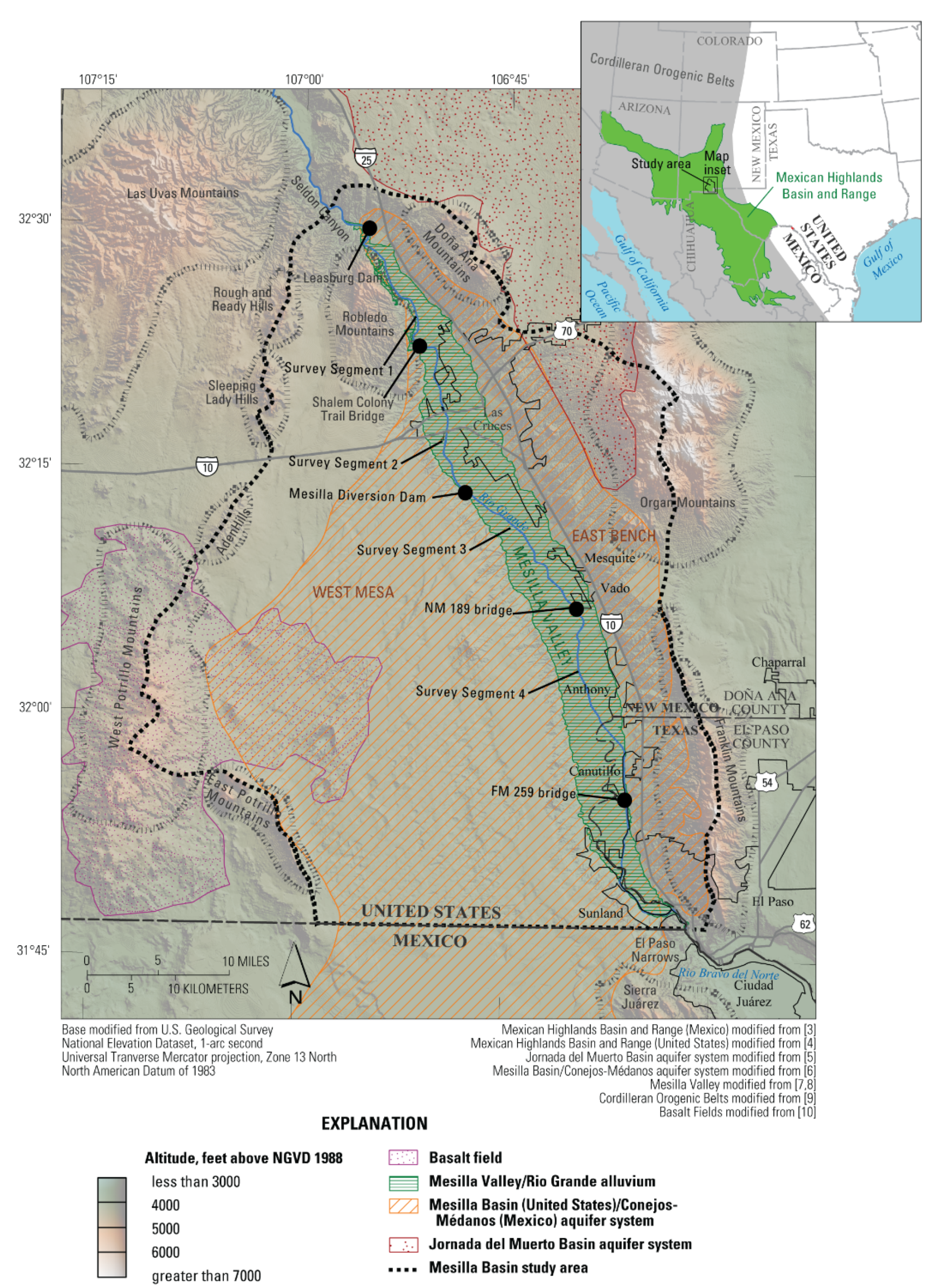
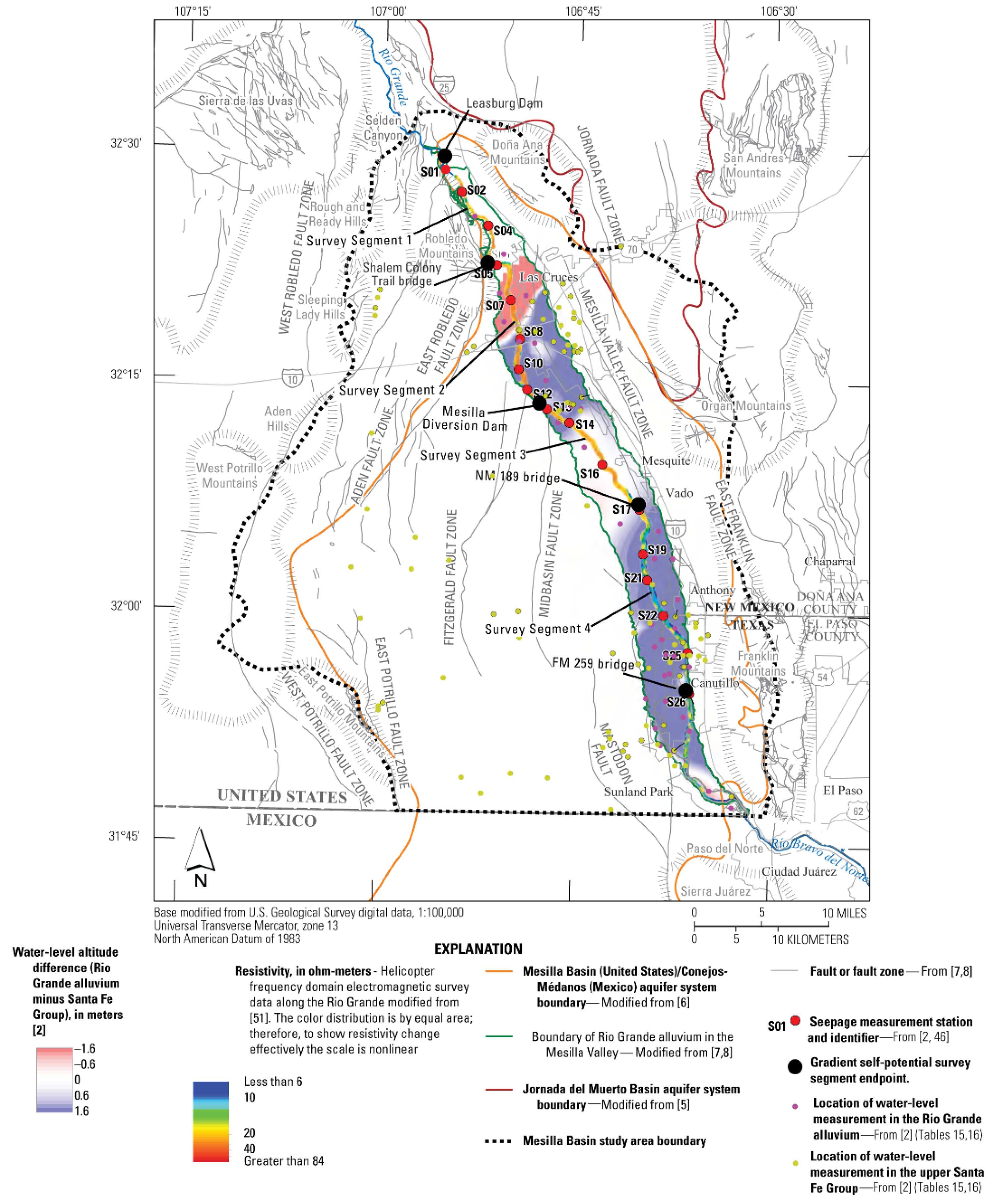
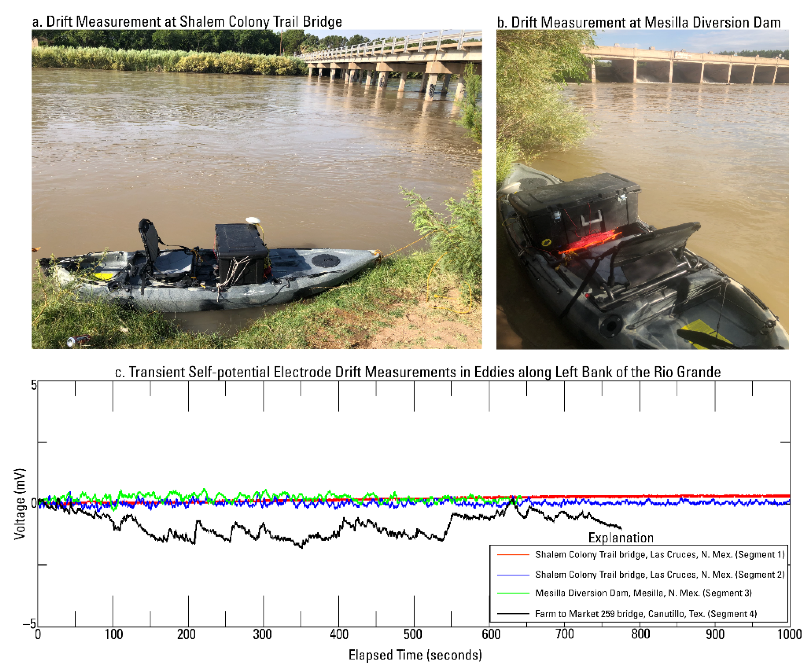
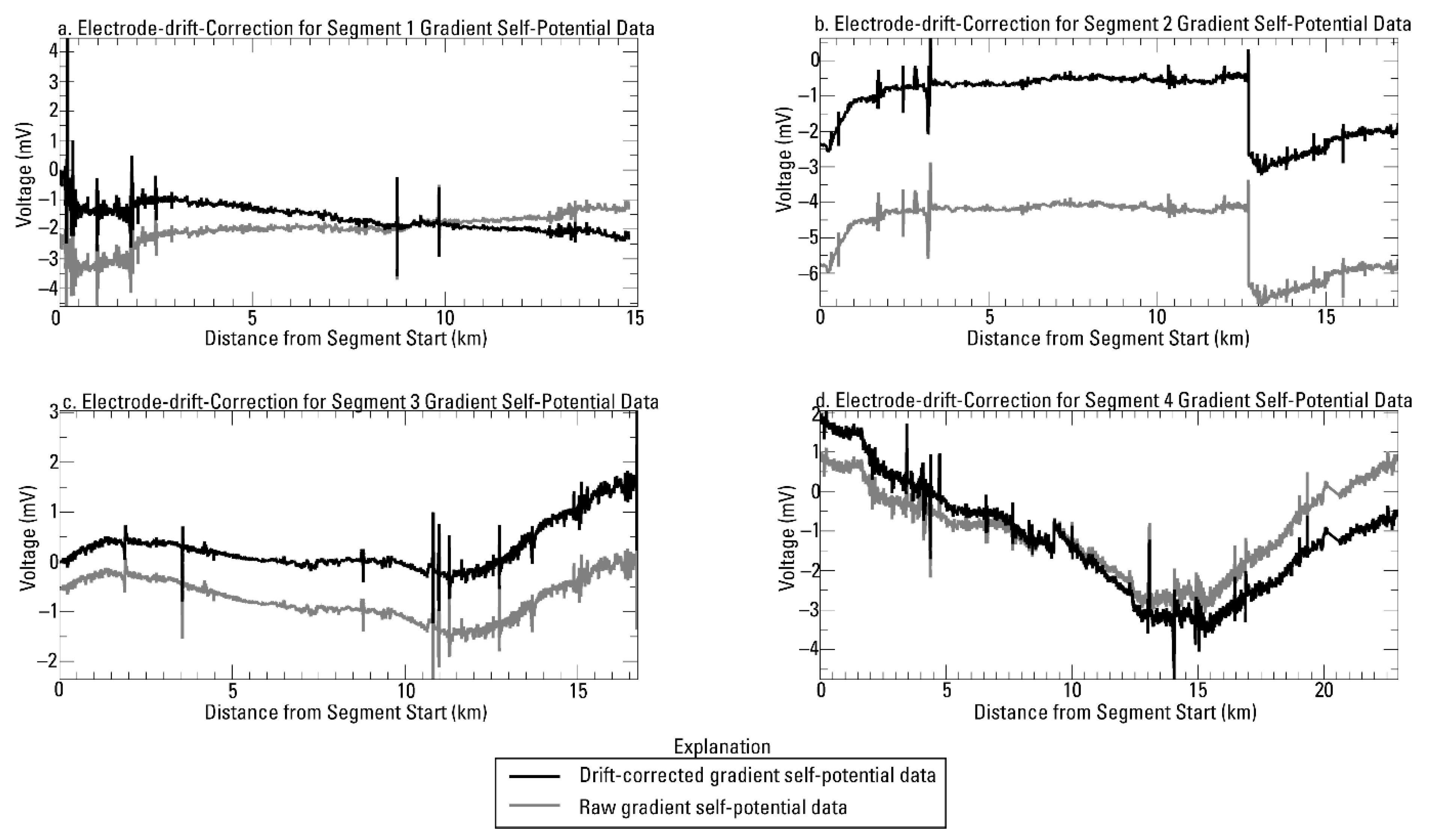
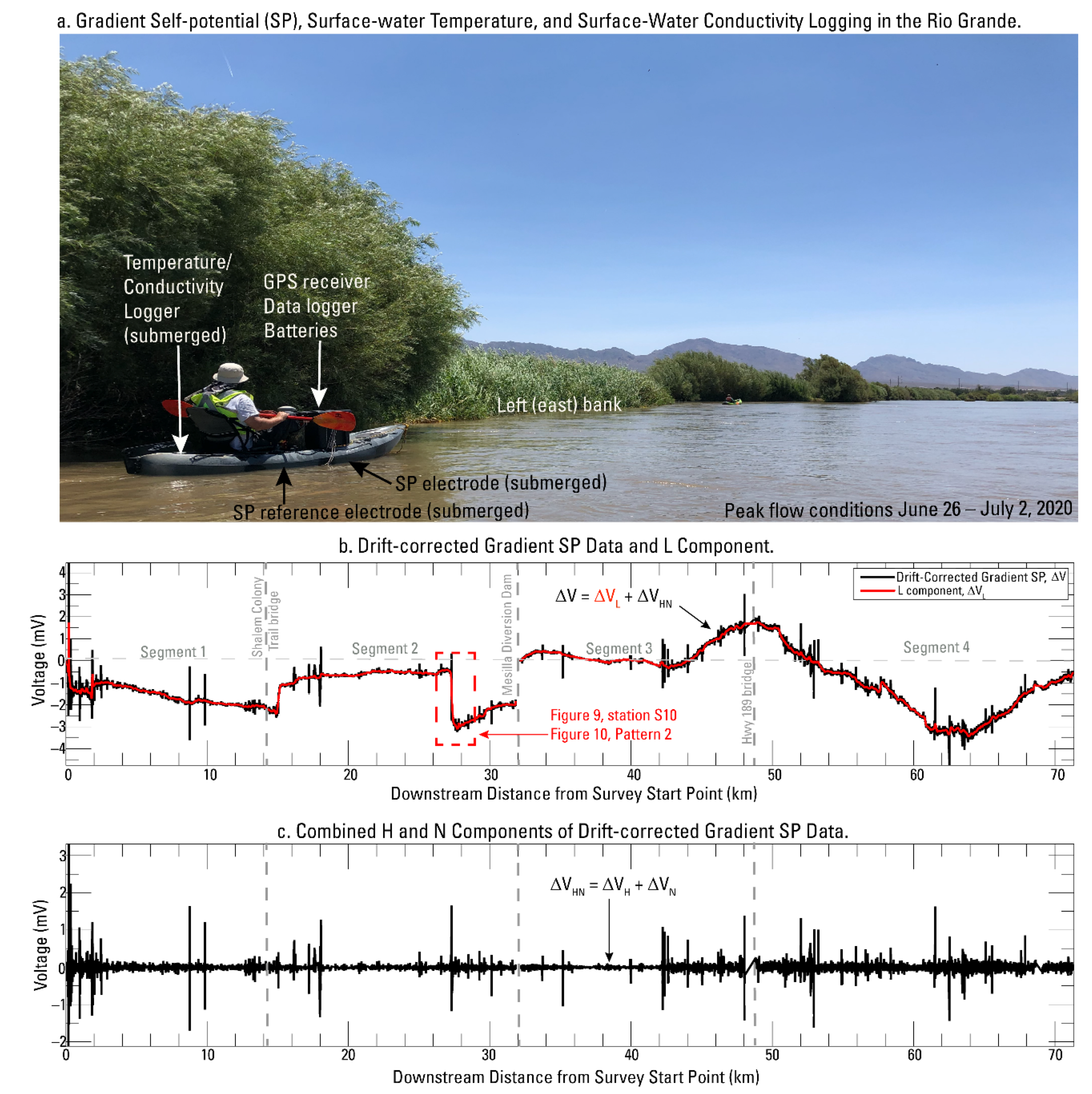
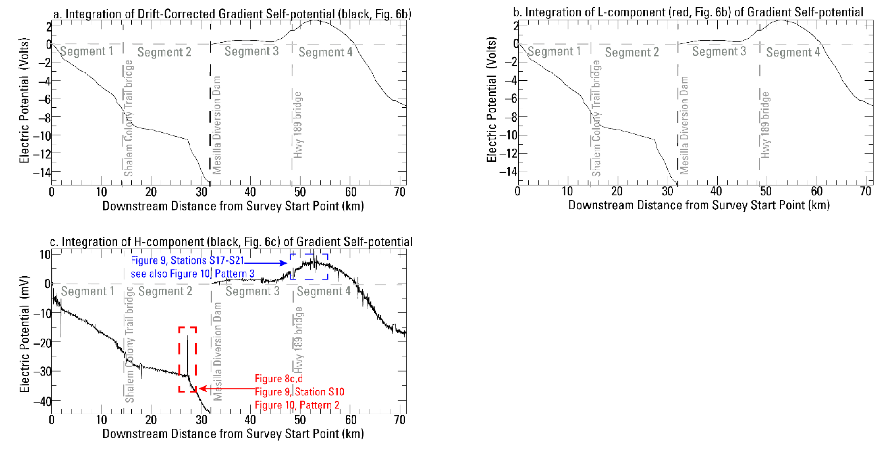
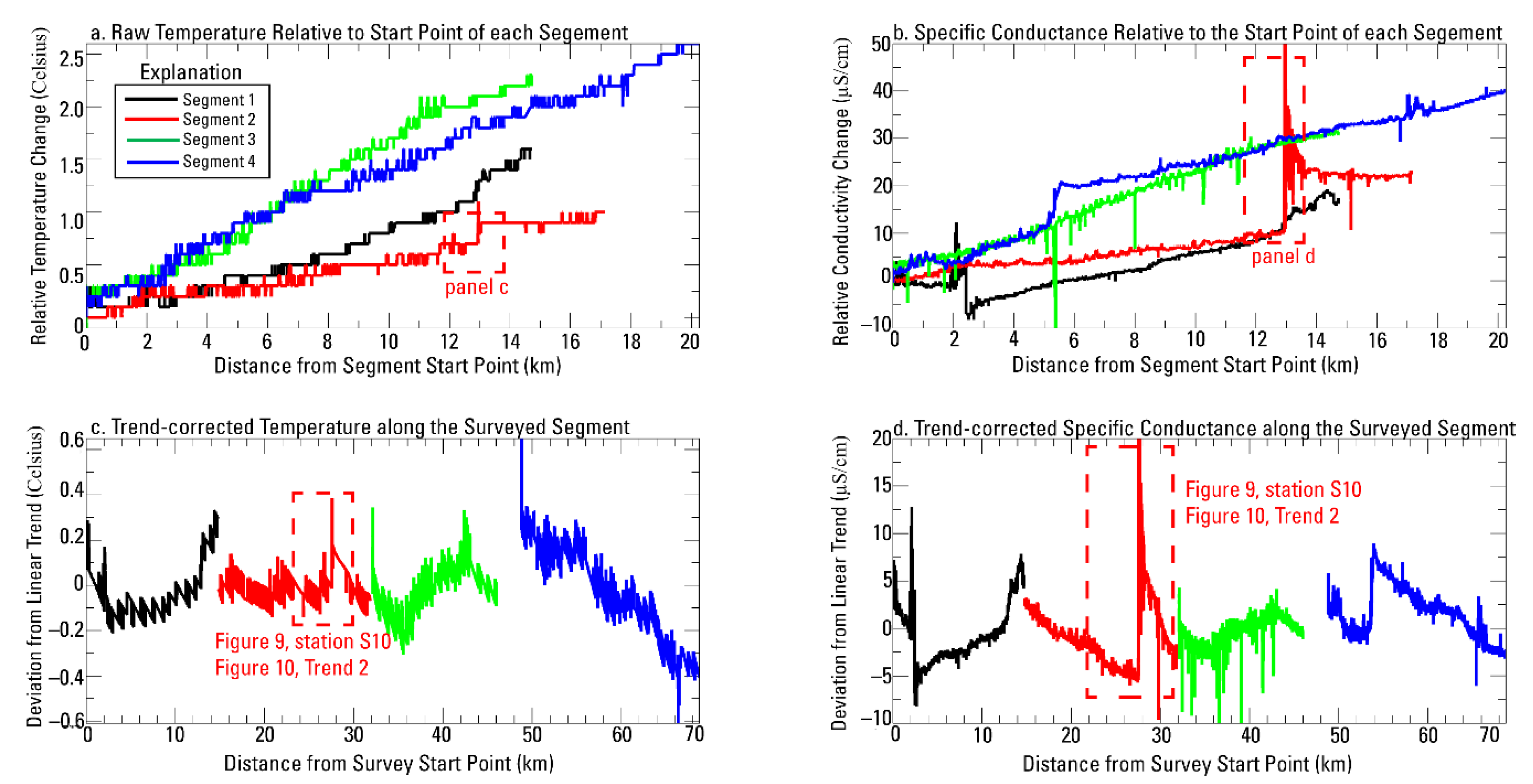
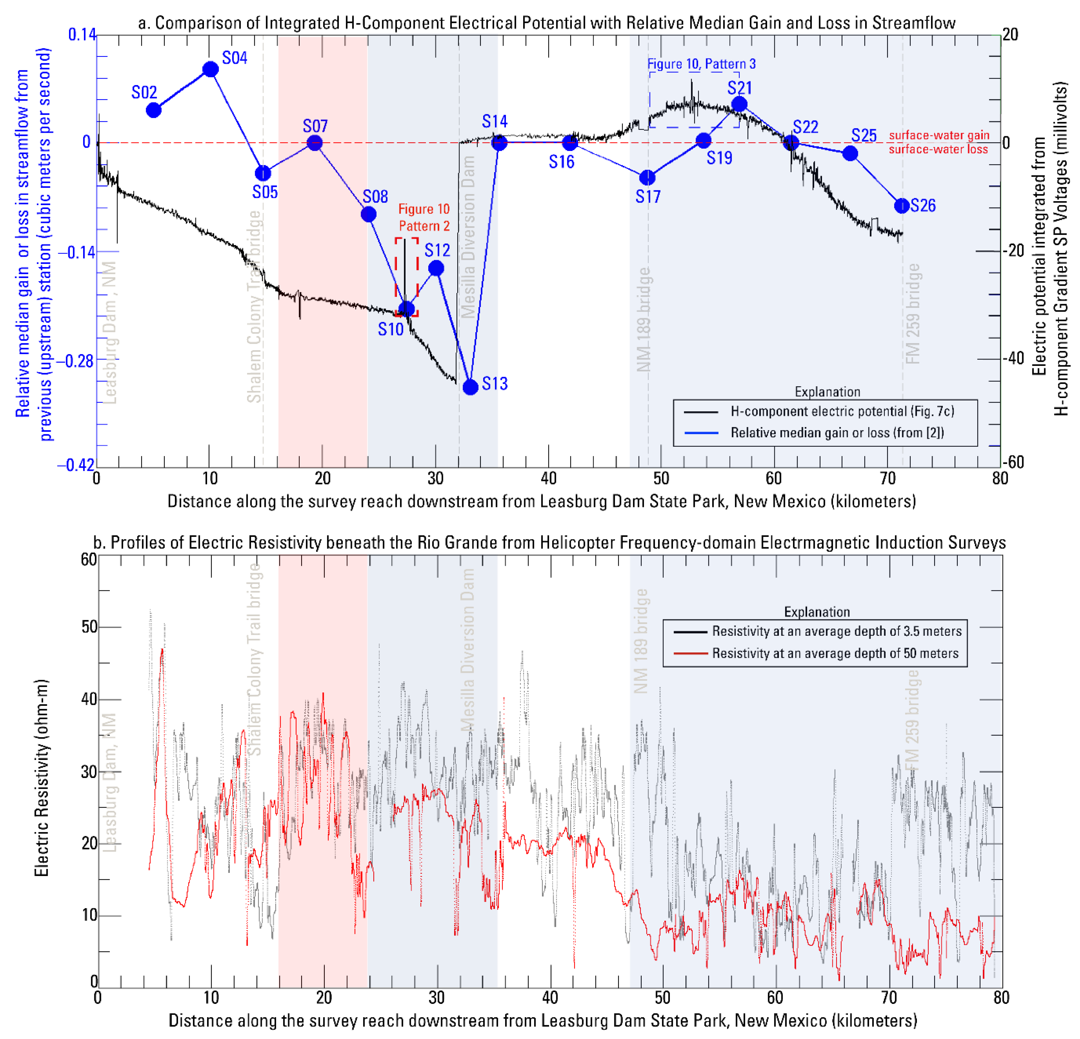
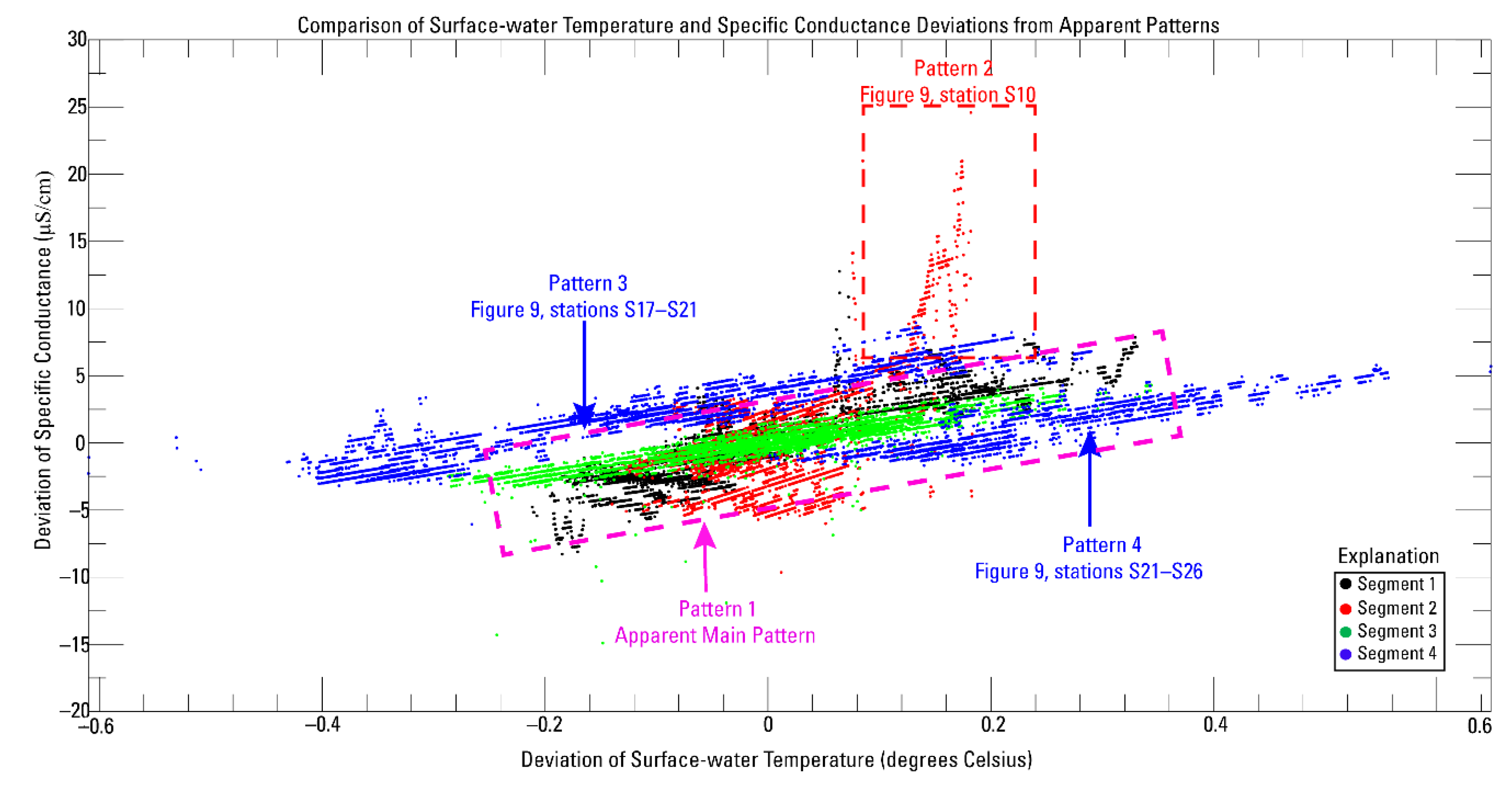
Table 1.
Summary of slopes, intercepts, and coefficients of determination from ordinary least squares (OLS) regression lines fitted to the gradient SP data (electrode drift voltage), surface-water temperature, and specific conductance.
Table 1.
Summary of slopes, intercepts, and coefficients of determination from ordinary least squares (OLS) regression lines fitted to the gradient SP data (electrode drift voltage), surface-water temperature, and specific conductance.
| Data Series | Survey Segment 1 | Slope | Intercept | Coefficient of Determination |
|---|---|---|---|---|
| Electrode Drift Voltage | 1 | 0.00035 | −0.00472 | 0.9556 |
| 2 | −0.00004 | 0.02242 | 0.0569 | |
| 3 | −0.00013 | 0.25666 | 0.0318 | |
| 4 | 0.0002 | −0.96317 | 0.0097 | |
| Surface-water Temperature | 1 | 0.00026 | 23.71262 | 0.9292 |
| 2 | 0.0002 | 22.60852 | 0.9717 | |
| 3 | 0.00045 | 22.33067 | 0.9758 | |
| 4 | 0.00035 | 22.71919 | 0.9939 | |
| Specific Conductance | 1 | 0.00304 | 623.7121 | 0.7115 |
| 2 | 0.00532 | 605.9887 | 0.7971 | |
| 3 | 0.00614 | 611.4147 | 0.9433 | |
| 4 | 0.00567 | 614.8888 | 0.9666 |
1 Survey segment 1: Leasburg Dam, New Mexico (N. Mex.) to Shalem Colony Trail bridge, Las Cruces, N. Mex. Survey Segment 2: Shalem Colony Trail bridge to Mesilla Diversion Dam, Mesilla, N. Mex. Survey Segment 3: Mesilla Diversion Dam to New Mexico State Road 189 bridge, Vado, N. Mex. Survey Segment 4: New Mexico State Road 189 bridge to Farm-to-Market 259 bridge, Canutillo, Texas (Figure 1, Figure 2 and Figure 3).
Publisher’s Note: MDPI stays neutral with regard to jurisdictional claims in published maps and institutional affiliations. |
© 2021 by the authors. Licensee MDPI, Basel, Switzerland. This article is an open access article distributed under the terms and conditions of the Creative Commons Attribution (CC BY) license (https://creativecommons.org/licenses/by/4.0/).
Share and Cite
MDPI and ACS Style
Ikard, S.; Teeple, A.; Humberson, D. Gradient Self-Potential Logging in the Rio Grande to Identify Gaining and Losing Reaches across the Mesilla Valley. Water 2021, 13, 1331. https://doi.org/10.3390/w13101331
AMA Style
Ikard S, Teeple A, Humberson D. Gradient Self-Potential Logging in the Rio Grande to Identify Gaining and Losing Reaches across the Mesilla Valley. Water. 2021; 13(10):1331. https://doi.org/10.3390/w13101331
Chicago/Turabian StyleIkard, Scott, Andrew Teeple, and Delbert Humberson. 2021. "Gradient Self-Potential Logging in the Rio Grande to Identify Gaining and Losing Reaches across the Mesilla Valley" Water 13, no. 10: 1331. https://doi.org/10.3390/w13101331
Note that from the first issue of 2016, this journal uses article numbers instead of page numbers. See further details here.