
An Enhanced Multi-Objective Particle Swarm Optimization in Water Distribution Systems Design
by
 , , , and
Mohamed R. Torkomany
1,2,* ,
,
Hassan Shokry Hassan
1,3,
Amin Shoukry
4,5,
Ahmed M. Abdelrazek
2 and
Mohamed Elkholy
2 1
Environmental Engineering Department, Egypt-Japan University of Science and Technology (E-JUST), New Borg El Arab City, Alexandria 21934, Egypt
2
Irrigation Engineering and Hydraulics Department, Alexandria University, Alexandria 11432, Egypt
3
Electronic Materials Researches Department, Advanced Technology and New Materials Research Institute, City of Scientific Research and Technological Applications (SRTA-City), New Borg El Arab City, Alexandria 21934, Egypt
4
Computer Science and Engineering Department, E-JUST, New Borg El Arab City, Alexandria 21934, Egypt
5
Computer and Systems Engineering Department, Alexandria University, Alexandria 11432, Egypt
*
Author to whom correspondence should be addressed.
Water 2021, 13(10), 1334; https://doi.org/10.3390/w13101334
Submission received: 8 April 2021
/
Revised: 4 May 2021
/
Accepted: 6 May 2021
/
Published: 11 May 2021
(This article belongs to the Special Issue Urban Water Networks Modelling and Monitoring)
Abstract
:The scarcity of water resources nowadays lays stress on researchers to develop strategies aiming at making the best benefit of the currently available resources. One of these strategies is ensuring that reliable and near-optimum designs of water distribution systems (WDSs) are achieved. Designing WDSs is a discrete combinatorial NP-hard optimization problem, and its complexity increases when more objectives are added. Among the many existing evolutionary algorithms, a new hybrid fast-convergent multi-objective particle swarm optimization (MOPSO) algorithm is developed to increase the convergence and diversity rates of the resulted non-dominated solutions in terms of network capital cost and reliability using a minimized computational budget. Several strategies are introduced to the developed algorithm, which are self-adaptive PSO parameters, regeneration-on-collision, adaptive population size, and using hypervolume quality for selecting repository members. A local search method is also coupled to both the original MOPSO algorithm and the newly developed one. Both algorithms are applied to medium and large benchmark problems. The results of the new algorithm coupled with the local search are superior to that of the original algorithm in terms of different performance metrics in the medium-sized network. In contrast, the new algorithm without the local search performed better in the large network.
1. Introduction
Designing water distribution systems (WDSs) has gained lots of interest in the past three decades. Despite the simple formulation of some of these problems, the feasible solutions are hardly identified because of the vastness of their search spaces. Moreover, the total enumeration of the solutions for this kind of problem is almost impossible [1]. For instance, if a small network consists of 20 pipes with only 5 available diameters in the market, the search space size of this network is around possible solutions. This complexity led to the necessity of using optimization methods to solve this type of optimization problem. Several optimization methods were applied on WDSs design such as linear programming (LP), dynamic programming (DP), non-linear programming (NLP), mixed integer programming (MIP), and evolutionary algorithms (EAs) [2,3]. Due to the vastness of search spaces and the discrete nature of variables for such problems, EAs began to take the lead because of their simplicity in execution and the quality of solutions they provide for such problems.
The complexity of WDS design problems increases when more components are added to the network pipes (e.g., pumps, storage tanks, etc.) since the search space gets wider [4]. The complexity also increases when more than one objective is considered because of the emergence of many feasible non-dominated solutions in this case and the trade-off between the different objectives functions [5]. For instance, the single-objective design of WDSs, which mainly depends on minimizing the capital cost, always results in a solution with minimum pipes diameters. However, this solution often produces the least hydraulic reliability of the network. When network reliability is added to the design as an objective, the conflicting nature between the cost and reliability affects the produced non-dominated solutions (i.e., the approximate Pareto set). In this case, decision-makers should select only one solution among these solutions for the real implementation of the network. Many other objectives may be added to these problems, such as minimizing the operational cost, maximizing water quality, and minimizing water leakage, to name a few. However, adding more than two objectives to the optimization problem usually forms an approximate Pareto surface of non-dominated solutions.
One of the most well-known meta-heuristic optimization algorithms used in designing WDSs is the particle swarm optimization (PSO) algorithm developed by Kennedy and Eberhart [6]. The algorithm is based on the swarm intelligence phenomenon, which may be observed in bird flocks or fish schools where a leader, which moves with the most convenient direction and speed, leads the whole swarm into a specific destination (this destination here is the optimum solution). Later, Coello and Lechuga [7] modified the PSO algorithm and developed the multi-objective PSO (MOPSO) algorithm by adding an external archive for saving non-dominated solutions (i.e., the approximate Pareto set) during the optimization process. Padhye [8] compared several proposals for archiving the particles in this external archive and stated the advantages and disadvantages of each method. He also proposed a new hybrid method by combining the -dominance and the sequential quadratic programming (SQP) search, and this method resulted in better convergent solutions.
PSO and MOPSO were frequently used in optimizing the design of WDSs and produced reasonable solutions compared to many other optimization algorithms, as will be explained subsequently. Wang et al. [9] made an extensive trial to obtain the best-known Pareto sets for twelve benchmark networks by accumulating the results of five evolutionary and hybrid algorithms so that those Pareto sets act as references for any other researchers. The hybrid AMALGAM algorithm, which includes parts of the PSO algorithm, and the non-dominated sorting genetic algorithm II (NSGA-II) had the most considerable contributions in forming the best-known Pareto sets of the studied networks.
El-Ghandour and Elbeltagi [10] made a comparison between five meta-heuristic EAs (the genetic algorithm (GA), PSO algorithm, the ant colony optimization (ACO) algorithm, the modified shuffled frog leaping algorithm (SFLA), and the memetic algorithm (MA)). They performed a single-objective optimization to design two benchmark networks, the two-loop network and New York tunnels network. The PSO algorithm proved to have the best performance among all other studied algorithms in terms of solutions efficiency and computational resources.
Additionally, Wang et al. [11] developed a hybrid algorithm called GALAXY to solve WDSs using six search operators including the main search operator of PSO, which is called the turbulence factor, TF. GALAXY’s results were superior compared to some baseline MOEAs, which were NSGA-II, -MOEA, and BORG algorithms. Monsef et al. [12] made a multi-objective optimization using NSGA-II, MOPSO, and the multi-objective differential evolution (MODE) of four benchmark networks (New York tunnel network, Hanoi network, Pescara network, and Modena network). MOPSO gave moderate result quality compared to the others while MODE algorithm surpassed all algorithms in terms of accuracy and computational resources.
MOPSO algorithm often performs well in WDSs design. It produces Pareto sets with functional diversities within the objective space; however, the convergence of final solutions is sometimes weaker than other algorithms [12]. Furthermore, MOPSO algorithm has few parameters to be tuned and has a fast-convergent search operator. It reaches sub-optimal solutions in relatively less computational time than other algorithms [10,12]. On the other hand, PSO algorithm, and the same applies for MOPSO algorithm, occasionally falls in local optima, severely suffering from premature convergence. Moreover, due to the non-linearity and non-convexity of the used objective functions in WDSs design problems, PSO and MOPSO particles may gather together at local optima, and the search process collapses [3,13].
Therefore, in a multi-objective WDS optimization, if MOPSO algorithm is improved in terms of convergence and diversity of the final solutions while taking advantage of its fast-convergent search operator, it can be superior compared to the other EAs frequently used in the literature. For this purpose, Different strategies may be added to hybridize the original MOPSO algorithm to improve its capabilities to reach near-optimal solutions when used to optimize WDSs design problems.
Although WDSs in many parts of the world are nowadays fully complete, in other parts (i.e., Middle East and some developing countries), they are still looking to improve their systems. Implementing new, robust, and yet simple algorithms for the optimal design of the networks would be essential. In this work, it is not intended to develop a new approach but to enhance the performance of MOPSO in terms of runtime convergence and solutions diversity compared to the original MOPSO while using a fixed computational budget in both cases. In addition, a comparison is held between the different strategies in the literature added to the algorithm and the effect of each on improving the overall performance is investigated. Two different benchmark networks are analyzed, and a comparison is held between the original and the modified MOPSO algorithms for each network. The structure of the rest of this paper is as follows: Section 2 describes the original MOPSO algorithm and its application to the design of WDSs. Section 3 identifies the performance metrics used in judging the results of each algorithm. Section 4 describes the strategies added to the original MOPSO algorithm to form the new algorithm. In Section 5, application of the local search to both MOPSO algorithms is described, while in Section 6 the used benchmark networks are illustrated. Finally, the obtained results and conclusions are given in Section 7 and Section 8, respectively.
2. Original MOPSO Algorithm
2.1. PSO Concept
The single-objective PSO imitates the idea of swarm intelligence. The algorithm initiates a population of particles representing a flock of birds or a school of fish aiming at moving towards the area of optimum solutions. The population initiation is usually done by generating random numbers for the decision variables (the decision variables are the pipes’ diameters in WDSs design problems) within their prespecified ranges. A decision vector is created for each particle, and the population consists of a prespecified number of population particles, . Thus, several decision vectors (, , …, , …, ) will be developed to form the initial positions of population particles. The algorithm starts to iterate to improve each particle position by following the swarm intelligence idea, as will be subsequently explained.
The objective function is evaluated for each particle. The algorithm saves the global best position of all particles () and the particles’ personal best positions (, , …, , …, ) for each particle in terms of the objective function value. Each particle position is improved in any following iterations by changing the velocity and direction as follows
where is the new particle velocity vector in iteration i+1, is the velocity vector in iteration i, is the inertia coefficient in iteration i that keeps the particle moving, and are random numbers between 0 and 1, is the cognitive parameter, and is the social parameter. In most studies, the values of and are set to 2.0 while may be calculated from several equations. One of the most common is
The new velocity vector of each particle should not exceed or drop below the maximum flying velocity vector, , and the minimum flying velocity vector, , respectively, so that the particle does not fly outside the search space [13]. is usually set as - and all values are typically set to 2.0 for all the particles.
Afterward, each particle position vector is updated according to the following equation
where is the new particle position in iteration i+1, and is the particle position in iteration i.
Then, the algorithm iterates within a prespecified number of iterations, , and at the last iteration is the optimum solution. A fixed total number of objective function evaluations, TNFE, to find the final solutions is adopted in this work. It represents the used computational budget in obtaining the results, i.e., the number of times the algorithm uses the simulator of the objective function, as will be explained later, to evaluate the fitness of all particles. The aim of fixing the TNFE, which should be proportional to the size of the problem search space, is to ensure an equal opportunity for this algorithm and any other version of it to find the final solutions using the same computational budget [9].
Coello and Lechuga [7] modified the single-objective PSO algorithm so that it acted like any multi-objective algorithm and developed the multi-objective PSO (MOPSO) algorithm. This transformation was done by adding an external archive/repository to save the non-dominated solutions every iteration. The leader of any iteration, which acts as for all population particles, is selected by the roulette-wheel selection [14] from the repository particles of the previous iteration. The repository has a maximum size, which equals the population size in this work, and if the repository is full, excess particles, which are selected using the roulette-wheel selection, are removed.
2.2. Formulation of WDS Design Problem
When solving the WDS design problems using MOPSO algorithm, each particle decision vector should represent all the pipe diameters in the network. The actual diameter of each pipe should be selected from a given set of the available diameters in the market. A hydraulic simulator is needed to obtain the pressure heads and flow velocities corresponding to each particle position. In this work, the hydraulic simulator is the freely available software EPANET2.0 [15]. MOPSO algorithm is written in a MATLAB Environment, and an EPANET-MATLAB toolkit is used to control EPANET2.0 from MATLAB [16].
The objective functions consist of minimizing network capital cost and maximizing network reliability. The network capital cost is a function of the cost of pipes, which is proportional to the number, length, and diameter of all pipes in the network according to the following equation
where NCC is the network capital cost, is the number of pipes in the network, is the unit cost per length of pipe k having an available diameter in the market , is the length of pipe k, and is the number of available diameters in the market.
On the other hand, the network reliability is measured by a surrogate measure, which is the network resilience [17]. The network resilience, , is a modification of the resilience index developed by Todini [18]. The resilience index expresses the surplus amount of available power for all network junctions to confront any failure, if any, happening in the network (e.g., pipes failure, contamination intrusion, etc.) considering the total power generated by reservoirs and pumps available in the network. The modification made by Prasad and Park [17] on the resilience index equation is adding a uniformity coefficient, U, for all junctions to check network redundancy. For more details, readers may refer to [17]. The network resilience can be calculated from
where varies between 0 and 1, is the number of junctions in the network, is the uniformity coefficient of junction m, is the demand of junction m, is the actual piezometric head of junction m, is the minimum required piezometric head for junction m and it is network-specific, is the number of reservoirs in the network, is the reservoir outflow, is the reservoir water elevation, is the number of pumps in the network, is the pumping power of pump p, and is the unit weight of water.
The uniformity coefficient for any junction m, , can be calculated from
where is the total number of pipes connected to junction m, and is the diameter of pipe t connected to junction m.
Values of the capital cost and network resilience are normalized to provide a fair probability of optimization for each objective function as follows
where NCC is the normalized value of network capital cost, is the normalized value of the network resilience, NCC is the minimum value of network capital cost, is the maximum value of the network resilience.
The original MOPSO algorithm is adapted here to find the pay-off characteristics curve (approximate Pareto set) between the network capital cost and the network reliability by running the algorithm several runs with different population sizes, and Pareto surfaces are identified. Finding the pay-off characteristics curve is done by identifying the non-dominated solutions saved in the external archive after finishing each run and by combining, ranking, and sorting the results from all runs. The different population sizes used for the required runs should be proportional to the size of the search space for each network. This proportionality is mandatory because small populations cannot perform well in a large search space due to their limited ability to discover the whole search space. In contrast, large populations, when used in a small search space, are computationally expensive. Consequently, large networks (i.e., a large number of junctions and pipes) require large population sizes and vice versa.
2.3. Constraints Handling
Two different types of constraints exist in WDSs design problems. The first type is a rigid constraint since it is related to satisfying the continuity and energy balance equations and it cannot be violated. This constraint is satisfied throughout the solution by using the hydraulic simulator, EPANET 2.0. The second type is a flexible constraint since it is related to the network operation and it might be violated. An example of this type is satisfying the required pressure heads of junctions and flow velocities of pipes within their prespecified limits.
Here, the flexible constraints are related to the pressure heads only and are handled using the same concept presented in [17]. After the end of each iteration during any run, the algorithm saves the non-dominated solutions, which are supposed to have zero constraints violations at the final iteration, in the external archive from population solutions. At any iteration, if a pair of sequential solutions (A) and (B) is selected from the population, solution (A) is saved in the repository while solution (B) is not saved if (i) solution (A) is feasible while solution (B) is infeasible; (ii) solutions (A) and (B) are both infeasible but solution (A) has less constraints violations compared to solution (B), or (iii) solutions (A) and (B) are both feasible but solution (B) is dominated by solution (A). After saving the new repository members, the repository is updated by repeating the same previous steps for the old and the new repository members, and an approximate Pareto front, PF, is obtained after the end of each iteration. Hence, the final approximate PF formed at the last iteration represents the best non-dominated solutions in a single run.
3. Performance Metrics
The need to measure the performance of multi-objective algorithms is essential for assessment and comparison purposes, especially in this work that aims at comparing two versions of the MOPSO algorithms, the original algorithm (OMOPSO) and the modified one (MMOPSO). Some metrics can be applied during the run (on-line metrics or runtime metrics), and others can be applied at the run end (off-line metrics). The runtime metrics are better in monitoring the performance of any algorithm, especially when information about the convergence speed is needed, as shown in [19]. The perfect performance of any multi-objective algorithm is achieved if it converges rapidly to the true PF while maintaining a diverse set of non-dominated solutions on the approximate PF.
Zitzler et al. [20] stated that the number of performance metrics should be equal to or greater than the number of objective functions to maintain theoretical accuracy. In this work, two runtime metrics are used, the runtime convergence metric [19] and the hypervolume metric [21]. The runtime convergence metric, , measures the Euclidean distances between each of the non-dominated solutions on the approximate Pareto set and the closest point on a reference set (e.g., the true PF). Then, it sums all these distances up and divides the summation by the number of non-dominated solutions. If this metric is close to zero, this indicates a good convergence of the generated approximate Pareto set.
On the other hand, the hypervolume metric, , measures both convergence and diversity of the obtained solutions. measures the objective space area which is covered by the non-dominated solutions in terms of a reference point. In this work, the reference point is selected to make the approximate PF of convex shape. The reference point, r, in this work is calculated as follows
where NCC is the maximum capital cost of the network, and is the minimum value of network resilience. NCC and NCC can be calculated by setting the maximum and minimum available diameter in the market for all the pipes in the network while and equal 1 and 0, respectively. is often classified as a monotonic measure since it does not depend on the true PF, unlike which needs a true PF [22]. In this work, the hypervolume value for the approximate PF is divided by the hypervolume value of the best-known Pareto set. Therefore, is converted to , which ranges from zero to one. If is close to unity, this means an excellent convergence and diversity of the generated approximate Pareto set.
In addition to and , the total number of non-dominated solutions, , for any final PF is utilized for displaying the intensity of this PF. In this work, is essential in presenting the effect of any strategy on the final PF intensity when it is applied to OMOPSO, as will be shown subsequently.
4. Modified MOPSO Algorithm
In WDS design problems, OMOPSO occasionally suffers from rapid convergence towards local minima during any single run, mainly if some repository members are concentrated in a particular area of the objective space. OMOPSO consumes a considerable amount of the number of function evaluations, NFE, to escape from local minima, thus reducing the opportunity to discover other areas of the objective space. Furthermore, the algorithm usually fails to maintain a diverse set of solutions, although it continuously seeks to improve diversity with the progress of iterations. Therefore, it often fails to obtain the whole set of non-dominated solutions located on the true PF and frequently loses competent solutions in terms of diversity during the archiving method. Consequently, there is a need to modify OMOPSO to escape from local optima and maintain or even increase its convergence and diversity rates to reach near-global optimum solutions. Many strategies are proposed here to enhance the overall algorithm performance by reducing the computational effort required for parameters tuning, improving the algorithm randomness during the search, and maintaining the best diverse non-dominated solutions obtained in any iteration. These strategies are explained in the subsequent sections. It should be noted that the PSO primary search operator is the same as that of OMOPSO (Equations (1) and (3)).
4.1. Self-Adaptive PSO Parameters Strategy
The main parameters of PSO are the inertia coefficient, , the cognitive coefficient, , the social coefficient, , and the maximum flying velocity, .
Firstly, many equations exist in the literature to calculate the value of , which keeps the particles moving during the whole run [23]. is implicitly responsible for switching the search from global search (exploration) at the beginning of the search into local search (exploitation) at the end of the search [24]. This switching is done by changing from its highest value in the first iteration (i.e., global search) to its lowest value (i.e., local search) at the last iteration. The highest and lowest values of in this study are assumed 1.0 and 0.5, respectively. Several equations of from [23] are used in trial runs. However, none of these equations dramatically affect the results of the WDS design problem, as also confirmed in [23]. Therefore, Equation (2) is kept the same in all the runs.
Secondly, the strategy of PSO self-adaptive parameters was proposed in [24] to eliminate the need for parameter tuning of , , and . The values of and usually vary from 0.2 to 4.0 while may be calculated as follows
where is a constant ranging from 0.1 to 1.0, and are vectors containing all the maximum and minimum limits of all the decision variables, respectively.
The self-adaptive parameters strategy is performed by assuming random values for , , and within their prespecified limits at the start of the search and by incorporating them within the decision vector for each particle to act like additional decision variables. Thus, the algorithm searches for the best values of these parameters until reaching their near optimum values. Their values differ from one particle to another and from one iteration to another. Although this method has a major drawback resulting from reducing the search quality because it increases the search space size, this strategy relieves the computational effort needed at the start of the solution to select appropriate values for these coefficients.
4.2. Selecting Repository Members Strategy
In this strategy, the repository members are selected from population particles to maintain the diversity of the non-dominated solutions set as much as possible. Following the original MOPSO algorithm, the leader of all particles in any iteration is chosen randomly from the repository using the roulette wheel selection method, thus providing an equal probability for each repository member to be the leader of the whole swarm.
On the other hand, the selection of the repository particles is performed using the non-dominated sorting, which was explained briefly in the constraints handling section. A problem occurs when the actual size of the repository (i.e., the number of saved members in the repository) exceeds its maximum allowable size. In OMOPSO, the excess particles are eliminated from the repository by selecting the exact number of particles that need to be eliminated using the roulette wheel selection method. This elimination method negatively impacts the quality of the approximate Pareto set since it may lead to losing eminent non-dominated solutions in terms of diversity. Accordingly, a modification is made to this elimination method by deleting the particles that would not adversely affect the achieved hypervolume of the approximate PF as much as possible. First, saved particles with the same position are removed, leaving only one particle for each repeated position. Then, excess particles, if any, are deleted one by one by while maximizing in each deletion. This strategy substantially helps in maintaining the resulted diversity of the approximate PF. Figure 1 summarizes the steps of this archiving strategy.
4.3. Regeneration-On-Collision Strategy
Surco et al. [3] used this strategy in a single-objective PSO optimization setting of WDSs design problems to prevent a PSO population from falling in local minima, hence jeopardizing the solution progress for the whole run. They explained the phenomenon of particles collision briefly. They stated that due to the non-linearity and the non-convexity of the total network cost function with penalties and the discrete nature of WDS design problems, any ordinary particle might collide with a local optimum in the objective space. Thus, the cognitive and social terms in Equation (1) equal zero for this particle. They also stated that if there is no criterion to fix the positions of the collided particles, this may lead to the assemblage of all particles in a local optimum and the occurrence of premature convergence.
Accordingly, a solution for this problem was developed in [3] by re-initiating any particle that collides with a local optimum while preserving the value of its flying velocity. Re-initiation of a collided particle position is done by generating a new random decision vector containing all the decision variables (i.e., all the diameters of network pipes) within their prespecified limits and keeping the same old flying velocity vector during the collision.
In the current work, a similar idea is adopted by re-initiating only one particle of any two collided particles within the objective space. The difference between this work and [3] is for two reasons: (i) to increase the probability of re-initiating any particle of any two particles that may have the same direction and therefore saving any consumed computational budget in their path to fall in any local minimum and (ii) to increase the leaping ability of the population in order to increase its efficiency in discovering the search space. Although this strategy may damage the convergence rate of the collided particles, it would help in preventing the MOPSO population from falling in local minima.
4.4. Adaptive Population Size Strategy
The population size has a double-edged nature in EAs since it affects the computational budget and both of the PF convergence and diversity of any run [25,26]. A small-sized population, although it consumes less computational budget, has less ability to perform a global search at the beginning of a run and thus may easily fall in local optima or obtain a final set of non-dominated solutions with low diversity. On the other hand, a big-sized population consumes more computational time with less progress in the overall convergence, although it may provide a proper final diverse set of solutions. Therefore, adopting a fixed population size throughout the whole run may lead to any of the previous problems.
Hence, the necessity of an adaptive-sized population arises. Chen and Zhao [25] tried this by adopting the ladder-concept where the whole iterations are divided into ladder steps with equal iterations in each step. In the first step, the largest prespecified population size is used. The population size remains fixed during any step; however, when moving from one step to another, the population size is changed according to the following rules: (i) if the diversity at the end of a step is less than a threshold value, the population size increases in the next step; (ii) if the diversity at the end of a step is more than a threshold value, the population size decreases in the next step, or (iii) if the diversity at the end of a step equals a threshold value, the population size remains the same.
In another study, Hadka and Reed [26] developed a new hybrid algorithm called Borg algorithm, where the population-to-repository ratio, also termed as the injection rate in some studies, was used to regenerate the population if a stagnation occurs in the population progress towards near optimum solutions. The population-to-repository ratio is usually above or equal unity. The idea of this ratio is to check the progress of population runtime convergence continuously. If there is no improvement in it after a prespecified number of iterations, the population is regenerated. Population regeneration is performed by combining the repository members and new members. These new members are generated from applying the mutation approach to the repository members.
Here in this work, both approaches of the two studies mentioned above are combined for better overall performance. The number of iterations, which is calculated based on the maximum population size, is divided into ten steps. Each step, T, comprises a fixed population and repository sizes. The population size has two bounds, which are the minimum population size, , and the maximum population size, .
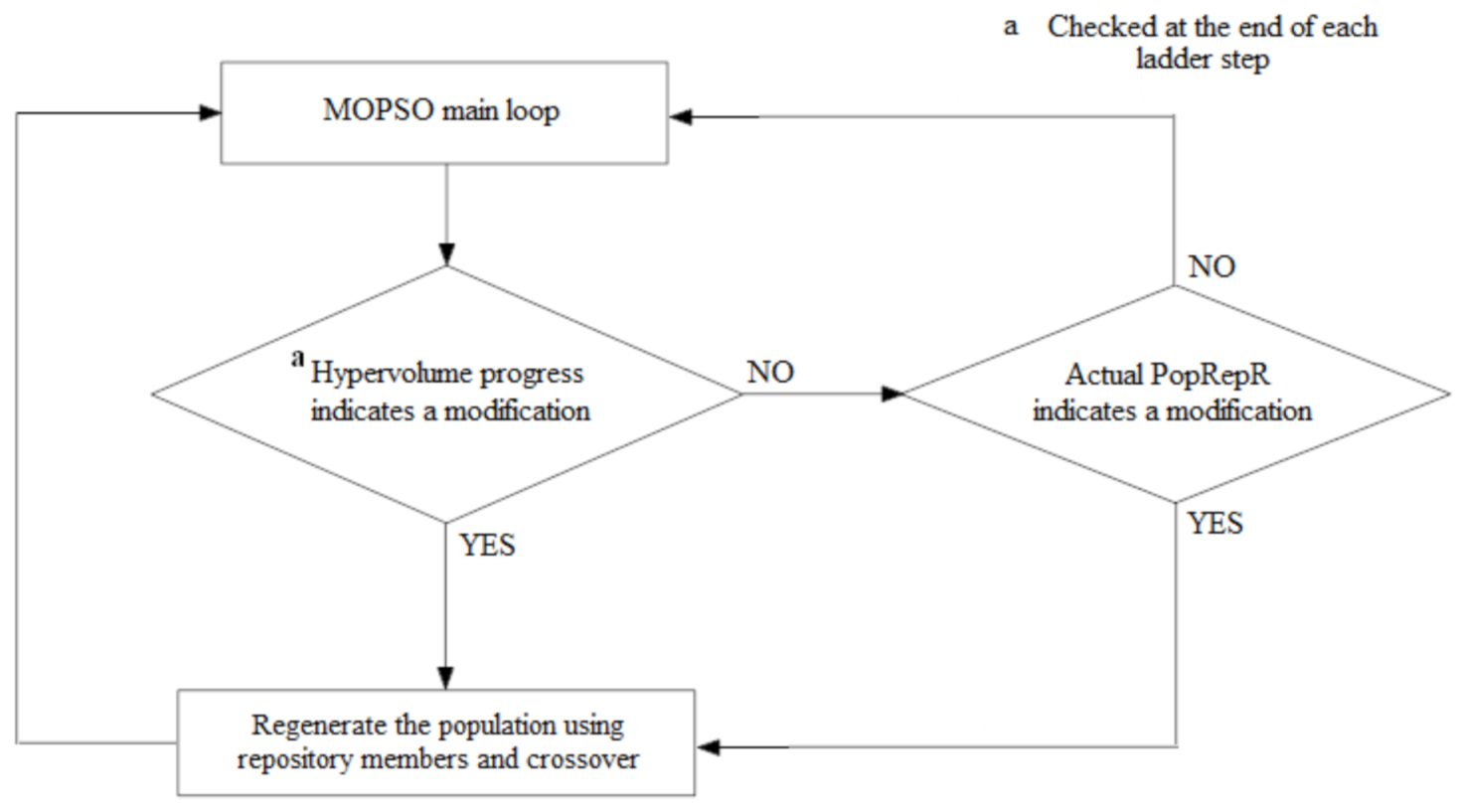
The population size is changed at each step end according to the following sequence. First, the average hypervolume throughout this step is checked. If there is no improvement in it in terms of a prespecified tolerance, the population is regenerated. It should be noted that the population regeneration is done according to a prespecified population-to-repository size ratio, . Otherwise, the actual is checked, and as in [26], if it is greater than the prespecified by 25%, the population is generated according to the prespecified . Figure 2 describes all the conditions that may lead to the regeneration of the population after the end of any single ladder step, T.
The population regeneration process is performed by assuming that the prespecified equals 1.0. Half of the new population matches half of the repository members’ positions and flying velocities. In contrast, the other half is generated by applying the crossover approach to the position and velocity vectors of each consecutive pair of repository particles. This strategy helps in relieving the computational effort needed for population size selection at the start of any run and increases the leaping ability of the population within the objective space during the search process.
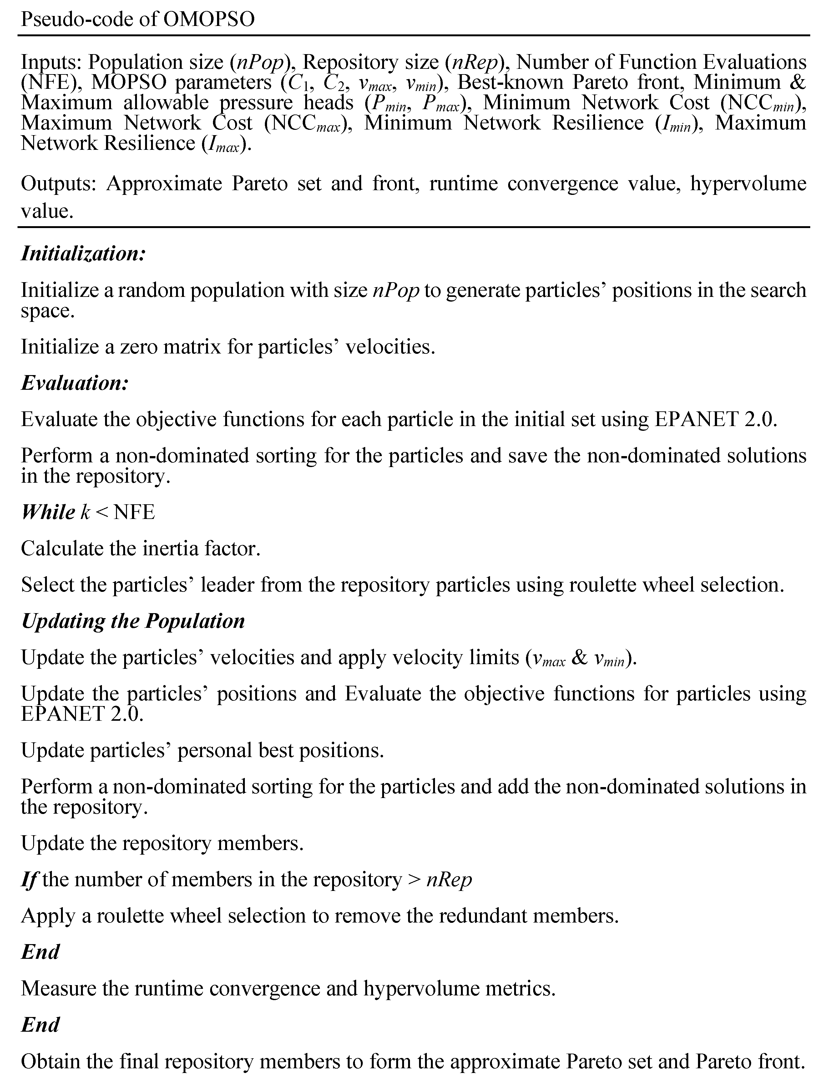
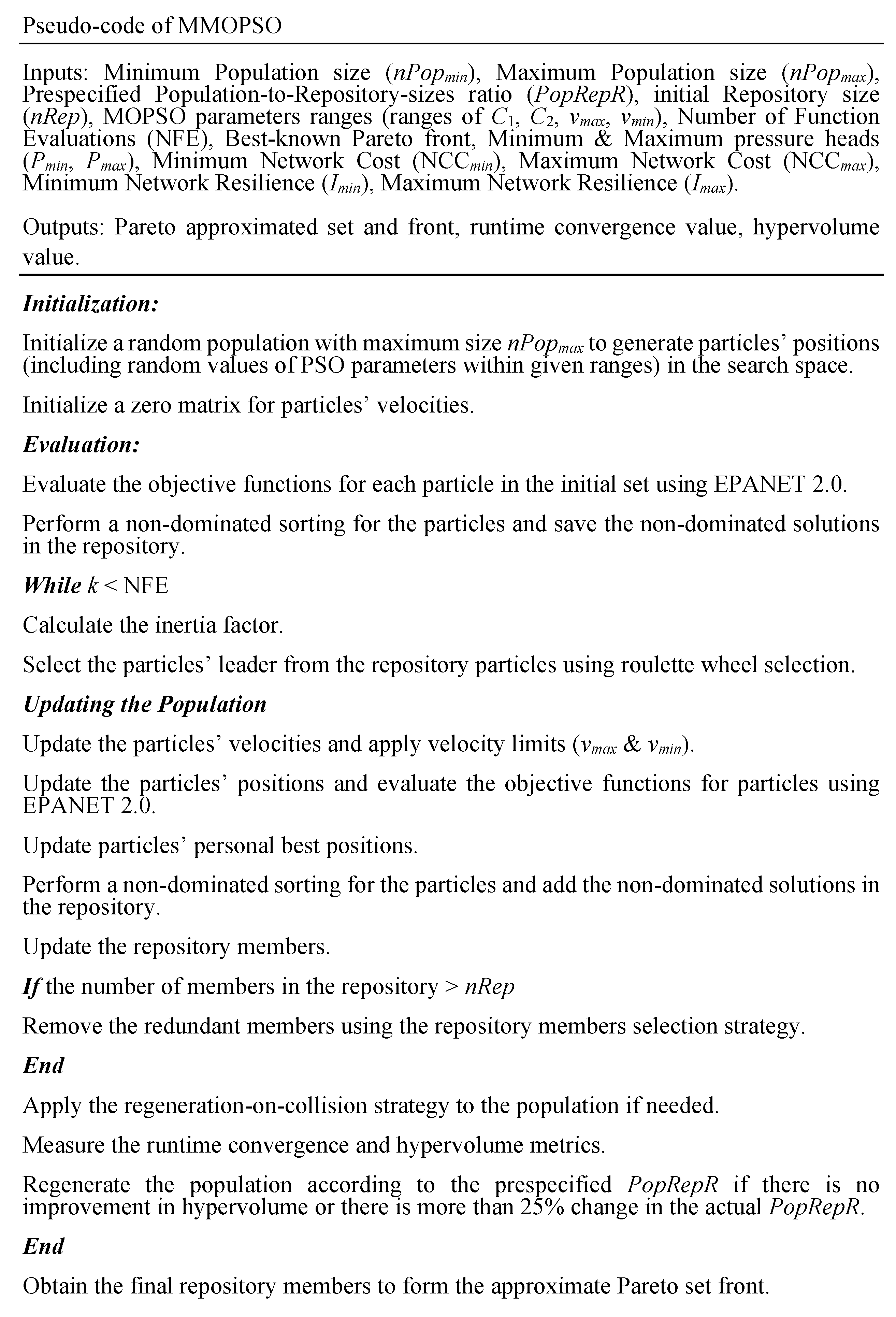
To conclude the previous sections, pseudo-codes for both OMOPSO and MMOPSO are presented in the appendix section (Figure A1 and Figure A2). Regarding the pseudo-code of MMOPSO, the self-adaptive PSO parameters are randomly initialized side by side to the decision variables at the initialization step. The step of updating repository members is performed by maintaining the achieved diversity of solutions. The regeneration-on-collision strategy is applied to the population particles at the end of each update of repository members. The population is resized using the adaptive population size strategy, which is performed periodically at the end of each ladder step as described before.
5. Local Search Application
A simple local search, LS, may be performed after obtaining any final PF from OMOPSO and MMOPSO to provide more local exploring ability to the search space areas adjacent to the obtained solutions. Here in this work, an LS method similar to that in [27] is used. Pipe diameters of any PF solution are separately and sequentially decreased two steps, if possible, to their least cost available diameters to form two new coupling solutions per each diameter in any solution. This step is repeated for all the PF solutions until all old solutions are locally explored. The new feasible solutions obtained from the LS, if any, are added to the old PF solutions, and a non-dominated sorting is performed to obtain an updated final PF. The LS step is applied for both OMOPSO and MMOPSO, resulting in four final PFs for any studied problem, which are the PFs of OMOPSO, OMOPSO with LS (), MMOPSO, and MMOPSO with LS ().
6. Benchmark Problems
Several benchmark problems regarding WDS design are found in the literature [9], and these problems may be classified into two main types, design problem and extended design (rehabilitation) problems. Two benchmark problems are used in this work; Hanoi (HAN) network [28] and Balerma irrigation network (BIN) [29]. Both HAN and BIN are design problems. HAN and BIN are selected to be representative of medium and large WDS, respectively. The size of each network is classified according to its search space size. The decision variables for HAN and BIN are designing 34 and 454 new pipes, respectively.
Table 1 contains the number of water reservoirs, , the minimum allowed pressure head above the ground level in meters, , the maximum permitted pressure head above the ground level in meters, , the minimum and maximum capital costs, NCC and NCC, in millions units, the number of available diameters in the market, , the minimum, intermediate, and maximum population sizes, , , and , respectively, used during the simulation runs, the total computational budget, TNFE, and the search space size for each network. The minimum allowed pressure head, , is network-specific. In contrast, the maximum permitted pressure head, , is assumed equal to the highest water level of all water reservoirs in each network. For more details about each network’s specifications, readers may refer to [9].
Wang et al. [9] obtained the best-known PF in the objective space for these networks in terms of network capital cost and network resilience by accumulating the results of five different algorithms. These PFs are used as reference sets, as illustrated previously in the performance metrics section. It is worth saying that Wang et al. [9] used an enormous total computational budget in their work to get the best-known PFs. For instance, in HAN, they used five different algorithms in 30 runs per each algorithm using NFE of 600,000. That is, 600,000 = 90 . While in this work, the total computational budget for HAN in any algorithm is around which is equivalent to only 2.24% of that used in [9]. The same applies for BIN in which the total used computational budget here is only which is 3.11% of that used in [9], which was . The success of this work relies on using very small computational budget to reach to near-optimum solution. This will guarantee the practicality of this approach.
7. Results and Discussion
7.1. A Comparison between the Proposed Strategies
A comparison is held using HAN network to investigate the effect of each proposed strategy when added to OMOPSO. Three runs are performed for each strategy using the population sizes mentioned in Table 1. Three similar runs are performed for OMOPSO and MMOPSO as well. The used NFE is 600,000 for any single run, and the maximum and minimum population sizes for the adaptive population strategy and MMOPSO are 60 and 240, respectively. The final values of , , and are obtained for the final PF of any run. The average values of , , and for each strategy/algorithm are presented in Table 2.
All the strategies indicate improvements in the values of , , and with respect to OMOPSO. However, the self-adaptive PSO parameters strategy records a lower average compared to OMOPSO, although it records improvements by almost 52.01% and 6.69% for the average values of and , respectively. This ensures that the value of is not always a good measure of the solutions’ convergence or diversity, since it only illustrates the density of the obtained PFs.
The most significant improvements in the average values of and among all occur in MMOPSO which include all the proposed strategies as shown in Table 2. MMOPSO records the highest relative improvements of about 68.45% and 13.25% of the average values of and in comparison with OMOPSO, respectively, regardless of the overlapping effect of the strategies. It is clear also that the strategy of the Adaptive Population size has significant effect compared to other self-standing strategies in improving the overall performance of the original MOPSO algorithm. For a user to select between applying this strategy or applying all of them in MMOPSO is a trade-off. It should be mentioned also that, HAN network has a relatively medium-sized search space, and if the aforementioned improvements are evident in HAN, the superior performance of MMOPSO is expected to be more obvious in BIN, which has a larger search space.
7.2. Results of the Different Proposed MOPSO Algorithms
For each of the used benchmark networks, the total computational budget, TNFE, is divided into four different stages; the main MOPSO search stage, which consumes around three-fourths of TNFE in HAN and two-thirds of TNFE in BIN, the main local search stage, which includes performing the local search two sequential times using the final PF obtained from the main MOPSO search stage, the secondary MOPSO search stage, which consumes around one-quarter of TNFE in HAN and around one-third of TNFE in BIN, and finally the secondary local search stage, which includes performing a local search only one time using the final PF obtained from the secondary MOPSO search stage. To ensure a fair comparison between all the proposed algorithms, it is worth noting that the used computational budget for the secondary MOPSO search stage for OMOPSO and MMOPSO equals the summation of the computational budgets that are consumed in the last three search stages for and , respectively.
Full details are presented here for the main MOPSO search stage since it represents most of the consumed TNFE in the two studied networks. In the main MOPSO search stage, OMOPSO runs 15 times using three different population sizes , , and , listed in Table 1 and by running each population size five separate runs. Furthermore, 15 more runs are also made for MMOPSO in each network, starting with as initial population size and bounded by .
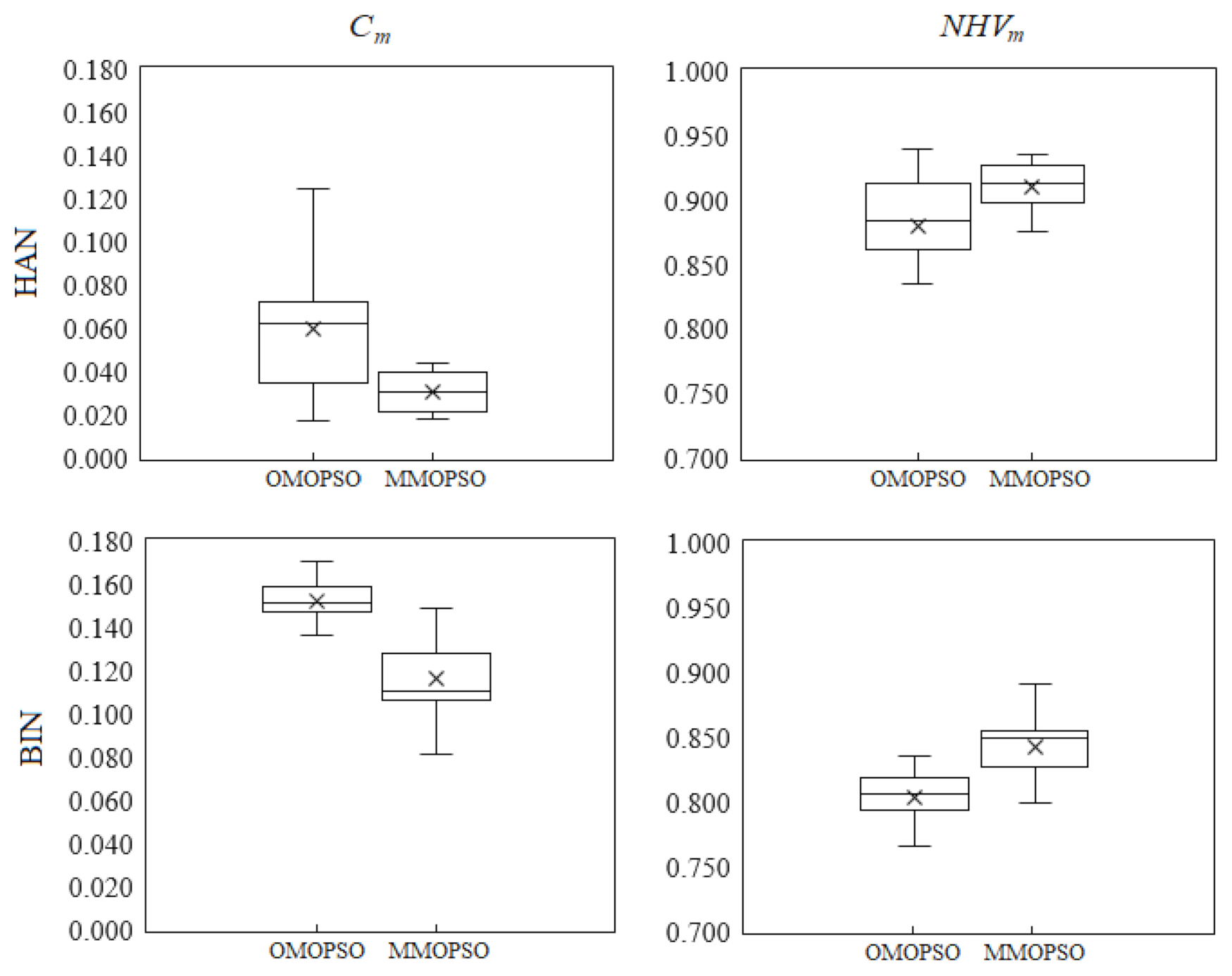
A statistical analysis is made to analyze the final values of and for each final approximate PF generated from each single run of OMOPSO and MMOPSO in the main MOPSO search stage. Box and whiskers plots are utilized to distinguish the differences in and for each network, as shown in Figure 3. In a box and whiskers plot, median and mean are represented by a central line and a cross sign within the box, respectively, the 25th and 75th percentiles are the edges of the box, and whiskers are the extreme points.
Recalling that lower represents improved convergence and greater represents both better convergence and diversity, an evident improvement is noticed in and for MMOPSO performance in HAN compared to OMOPSO. The 50.57% and 48.74% relative decreases are found in the median and the mean values and almost 3.36% and 3.46% relative increases in the median and the mean values, respectively.
A better performance of MMOPSO in terms of is also outlined in BIN since the relative increase in ’s median and mean are 5.30% and 4.82%, indicating the quality of MMOPSO searching process in big search spaces compared to OMOPSO. The relative decrease in ’s median and mean are 27.11% and 23.28%.
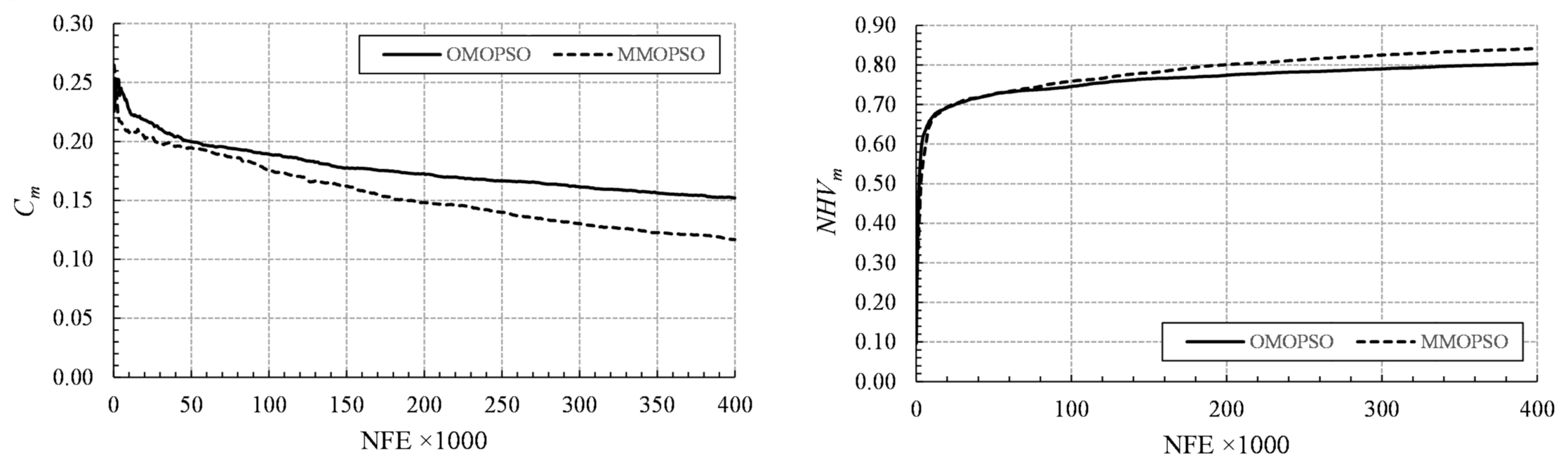
Moreover, the runtime performance of and metrics for both networks may be detected by tracking their values during any run. The average curves of the runtime performance metrics, and , for each algorithm in BIN network, which is the most difficult network with respect to the search space size, are shown in Figure 4. MMOPSO frequently succeeds in converging to better final values of and , producing a better quality of the final set of non-dominated solutions. Moreover, MMOPSO converges faster towards the area of near-optimum solutions compared to OMOPSO.
Regarding the self-adaptive PSO parameters (which are , , and ), a statistical analysis is also made to clarify their values for each non-dominated solution set obtained from each run from the overall 15 runs, as shown in Figure 5. It may be noticed that the mean values of in HAN and BIN are 0.2970 and 0.4959 while the mean values of and are 1.8529 and 1.9365, and 0.7247 and 0.8965, respectively. Subsequently, the variation in these values indicates the significance of the self-adaptive PSO parameters strategy since it alleviates the complexity of parameterization needed for investigating the best values of these parameters at the beginning of any run.
In the strategy of selecting repository members, MMOPSO continuously succeeds in saving only dissimilar non-dominated solutions during any run. It keeps only non-dominated solutions that maintain the acquired hypervolume from previous iterations. Although this strategy helped in providing a unique set of non-dominated solutions in HAN, it did not function in BIN because of the difficulty of finding a high number of non-dominated solutions that exceeds the maximum repository size during any single run. For example, in one of the best HAN runs in terms of its final value using OMOPSO, the final repository is found full of 60 non-dominated solutions. Still, 5 of them are similar, leaving only 55 unique solutions. On the other hand, in one of the best runs of MMOPSO in HAN in terms of its final as well, the repository saved 145 unique solutions without any duplication. Additionally, due to the large search space of BIN, OMOPSO saves 125 solutions without repeat in the best run in terms of while MMOPSO saves 273 unique solutions.
Furthermore, it is noticeable that the regeneration-on-collision strategy rarely occurs while used in BIN. This low probability of collision between particles is due to the enormous search space of this network, unlike HAN in which the regeneration-on-collision strategy frequently occurs during each run. Although the collision between particles is a function of the maximum population size, the minimum population size, and the search space size, the search space size proved to have significant effect in this rare occurrence of particles collision in BIN. In HAN, the mean number of total collisions reaches 5689 collisions with a standard deviation of nearly collisions. On the contrary, almost all the runs in BIN record zero collisions between particles. Thus, the regeneration-on-collision strategy significantly expresses its ability to prevent the population from falling in local minima in only medium search space problems. For large search space problems, the vastness of the available solutions and the breadth of the search space overwhelmingly decrease the probability of collision between any of the particles to a great extent.
Eventually, the adaptive population size strategy helps in preventing the modified algorithm from being stagnant during the search progress of any run. This strategy helps in changing the whole geometry of the population if there is no sensible improvement in values. Thus, this strategy helps in increasing the population leaping ability within the objective space, providing more opportunity to discover the search space. This previous behavior is in contrast with OMOPSO in which the population is usually gathered in close positions and follows a random leader every iteration to desperately increase its ability to move towards undiscovered regions of the search space. Moreover, this strategy switches frequently between large to small population sizes and vice versa during any run to make the most beneficial use of the available computational budget, NFE. The strategy starts using a large population size at the beginning of the search and then reduce the size in the middle of the search process to increase the local search ability. During one of the best runs in BIN in terms of using MMOPSO, the population size starts with the maximum size of 800 particles to provide a good exploration opportunity for the algorithm. Then, after consuming around a quarter of the computational budget, the population size dramatically decreases to be around only 145 particles from the quarter to the three-fourths of the computational budget to provide a good exploitation opportunity. After that, it slightly increases to reach 245 particles in average to provide more storage capacity for the repository for the rest of the run.
The final non-dominated feasible solutions, which are obtained from 15 runs for any algorithm, are used to obtain approximate PFs of each network as follows. The final non-dominated solutions from all runs are accumulated, ranked according to their network resilience value, and sorted using the non-dominated sorting to form only one final approximate PF per each network. Table 3 and Table 4 summarize the final values of and for the final approximate PFs generated from each algorithm in HAN and BIN, respectively, in the main MOPSO search stage and the subsequent search stages.
Differences between OMOPSO and MMOPSO are evident in the main MOPSO search stage in HAN since MMOPSO is more capable of exploring the search space compared to OMOPSO. The final number of non-dominated solutions, , for the approximate PF in HAN is 166 solutions for OMOPSO and 242 solutions for MMOPSO. Moreover, the final values of and for MMOPSO approximate PF are improved by 25.42% and 2.54%, respectively, compared to the approximate PF of OMOPSO.
MMOPSO significantly expressed its superiority in BIN in the main MOPSO search stage since the modified algorithm reaches extreme solutions in terms of the value of objective functions with more convergence values in terms of the reference PF compared to OMOPSO. for the accumulated approximate PF in BIN is 151 for OMOPSO and 289 for MMOPSO. Improvements in and are 36.96% and 6.46%, respectively, in comparison between MMOPSO and OMOPSO.
In the main LS stage, obvious differences start to take place between OMOPSO and MMOPSO, and their versions with local search, and , respectively. The LS is performed twice using the final PF obtained from the main MOPSO search stage. In HAN, and are improved by 65.54% and 2.45% for , and by 59.09% and 1.72% for , respectively, with respect to their values in the previous search stage. increases as well from 166 to 234 for and from 242 to 298 for , respectively.
Whereas in BIN, the most significant impact of this stage is intensifying the number of non-dominated solutions of the final PF, , while recording minor progress in terms of and . increases from 151 to 808 and from 289 to 2655 for and , respectively.
In the last two search stages for and , a secondary MOPSO search is performed and followed by a secondary LS search. In HAN, all the performance indicators, which are , , and , improved to be 0.0051, 0.9840, and 276 in the secondary MOPSO search stage and to reach 0.0039, 0.9903, and 312 in the secondary LS search stage, respectively, for . The same applies for in which , , and improved to reach 0.0053, 0.9896, and 319 in the secondary MOPSO search stage and 0.0041, 0.9917, and 363 for the secondary LS search stage, respectively.
In BIN, expresses its superiority over since it reaches a better final set of non-dominated solutions in terms of all the performance indicators. reaches 0.0695, 0.9193, and 5455 for , , and after performing the secondary MOPSO search stage and the secondary LS search stage compared to 0.0956, 0.8931, and 741 for after performing the same two search stages.
The accumulated computational budget used in the last three search stages for and are used to perform an extended optimization using OMOPSO and MMOPSO in the two studied networks. OMOPSO reaches 0.0066, 0.9860, and 193 and MMOPSO reaches 0.0122, 0.9730, and 234 for , , and , respectively in HAN. The previous results confirm the superiority of over all the other studied algorithms in HAN.
While in BIN, OMOPSO reaches 0.0966, 0.8783, and 149 and MMOPSO reaches 0.0483, 0.9321, and 399 for , , and , respectively, after extending the optimization that is performed in the main MOPSO search stage. Surprisingly, MMOPSO outperformed and all the other studied algorithms which indicates the priority of MMOPSO and the insignificance of performing an LS in large WDSs, especially in terms of and .
Generally, the LS increases for the algorithm by 23.14% after the main MOPSO search stage and by 13.79% after the secondary MOPSO search stage in HAN. The same applies for BIN in which the local search increases for by 818.69% after the main MOPSO search stage and by 498.79% after the secondary MOPSO search stage.
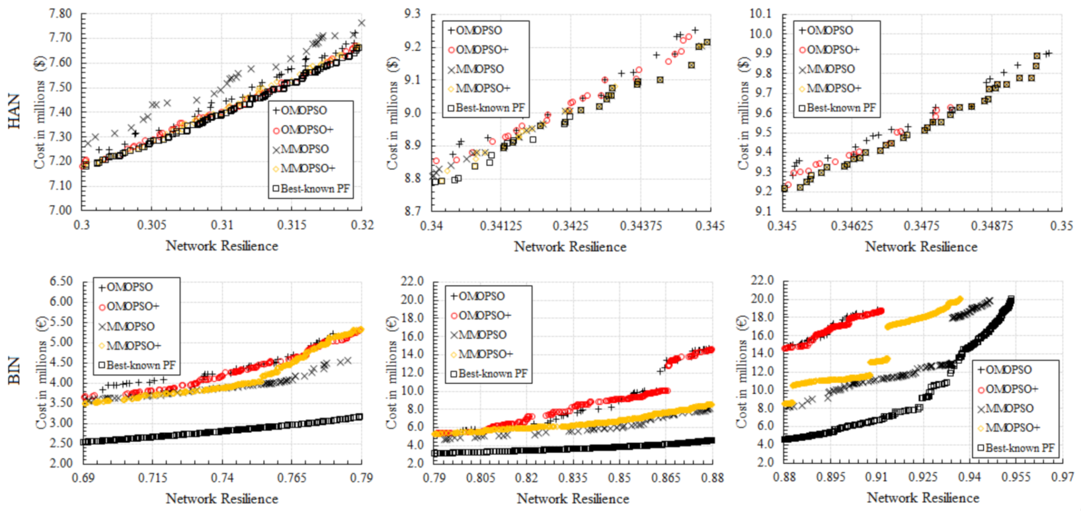
Parts of the final PFs for all algorithms in both networks after the end of all search stages are shown in Figure 6. Generally, all OMOPSO and MMOPSO studied versions fail to reach the full reference PFs in HAN and BIN despite its improved performance. This failure is undoubtedly due to the use of only one algorithm to obtain the results instead of accumulating the results of five different algorithms while using an enormous total computational budget in [9] to obtain the best-known PFs for HAN and BIN.
The enhanced performance of MMOPSO is evident compared to OMOPSO for several reasons:
- A reduced effort is needed for parameterization of PSO since the self-adaptive PSO parameters strategy nearly optimizes their values during the search process.
- Implementing the regeneration-on-collision strategy prevents the population from being trapped in local minima areas and this strategy is more evident in medium-sized networks.
- More leaping ability is provided to MMOPSO by depending on the regeneration-on-collision and the adaptive population size strategies. The random changes of some or all particles’ positions during the search process substantially help in discovering new solutions areas within the search space.
- The real dilemma of whether to use a relatively large or relatively small population size is alleviated by depending on the adaptive population size strategy. This strategy strengthens the global search at the beginning of the search and the local search at its end.
- The local search strengthens the local exploration ability of MMOPSO in medium sized problems since it investigates nearly all the local solutions around the gained non-dominated solutions of MMOPSO final PF, providing a good opportunity to increase the available design choices for decision makers upon the real implementation of networks.
However, MMOPSO still needs further improvements to be capable of capturing the whole set of non-dominated best-known solutions using a minimized computational budget. The leader selection criterion and the random initiation of the population at the search beginning should be improved so that MMOPSO becomes more efficient in exploring the whole search space.
8. Conclusions
Several strategies are proposed, and each is tested and implemented to modify and upgrade the original MOPSO algorithm for faster convergence with small computational time. These strategies include the self-adaptive PSO parameters strategy, the new archiving system to save repository members, the regeneration-on-collision strategy, and the adaptive population size strategy. In addition, a simple local search method is applied twice to the original and the modified MOPSO algorithms to examine the ability of local search on both thus creating a total of four different MOPSO algorithms; OMOPSO, MMOPSO, OMOPSO with local search (), and MMOPSO with local search (). The algorithms are tested on two benchmark problems, HAN and BIN, which represent medium and large search space problems, respectively. Results of all the studied algorithms are compared in terms of three performance metrics which are the runtime convergence metric, , the hypervolume metric, , and the number of obtained non-dominated solutions, , indicating significant improvements in and for the modified algorithm and its superiority in convergence compared to the original one.
Results for the different applied strategies showed that the self-adaptive PSO parameters strategy relieved the computational efforts at the beginning of runs since it merged the PSO parameters within the search process, converging them to their near-optimum values. The new archiving system of repository members and the regeneration-on-collision strategy improve the search process in the medium search space problem by preserving the maintained diversity and preventing the population from falling into local minima. However, in the large search-space problem (BIN network), they were not functioning. In contrast, the adaptive population size strategy improves the search process in all the studied problems by resizing the population according to the overall progress in , thus making a better usage of the available computational budget.
The local search, which is performed two times between the two MOPSO search stages and one time at the end, proved its efficiency in intensifying any final approximate Pareto set obtained from both of the main and the secondary MOPSO search stages. The local search usually increases the number of non-dominated solutions when applied after any MOPSO search stage.
Although the modified MOPSO algorithm combined with the local search () provides a superior final set of solutions in HAN, the modified MOPSO algorithm without the local search, MMOPSO, proved its priority in BIN, indicating the insignificance of conducting a local search in large WDSs designs in the way to reach a more convergent and diverse set of solutions. Despite the improved performance of the developed MOPSO algorithm, further benchmark networks and real networks with different objectives (e.g., operational costs, water quality) and additional decision variables (e.g., location, size and number of storage tanks, optimum pumping power) should be tested to ensure the applicability of the novel algorithm.
Author Contributions
Conceptualization, M.R.T.; methodology, M.R.T.; validation, M.R.T., A.M.A., M.E.; investigation, M.R.T., M.E.; data curation, M.R.T., M.E.; writing—original draft preparation, M.R.T.; writing—review and editing, M.R.T., H.S.H., A.S., A.M.A., M.E.; visualization, M.R.T.; supervision, H.S.H., A.S. All authors have read and agreed to the published version of the manuscript.
Funding
This research received no external funding.
Institutional Review Board Statement
Not applicable.
Informed Consent Statement
Not applicable.
Data Availability Statement
The used data in this study are available as follows: All the EPANET 2.0 input files, the best-known Pareto fronts [9], and descriptions of the used networks may be found at the following link (http://tinyurl.com/cwsbenchmarks/) (accessed on 10 May 2021). The original MATLAB source code of the MOPSO algorithm may be found on the website of Yarbiz project via (https://yarpiz.com/59/ypea121-mopso) (accessed on 10 May 2021). The MATLAB codes of OMOPSO and MMOPSO accompanied with a tutorial to explain their usage in the studied benchmark problems are found at (http://dx.doi.org/10.17632/39xmcn87d9.1) (accessed on 10 May 2021).
Acknowledgments
The first author would like to thank the Ministry of Higher Education (MOHE) in Egypt for providing the computational resources and the technical support needed for this work. We also thank Qi Wang for his cooperation in checking the resilience calculations in large networks. The first author would also like to thank the Centre of Water Systems at the University of Exeter for providing a brief description for all the benchmark problems used in this work.
Conflicts of Interest
The authors declare no conflict of interest.
Appendix A. Pseudo-Code for OMOPSO Algorithm
Figure A1.
Pseudo-code of the OMOPSO algorithm in a single run.

Appendix B. Pseudo-Code for MMOPSO Algorithm
Figure A2.
Pseudo-code of the MMOPSO algorithm in a single run.

References
- Marchi, A.; Salomons, E.; Ostfeld, A.; Kapelan, Z.; Simpson, A.R.; Zecchin, A.C.; Maier, H.R.; Wu, Z.Y.; Elsayed, S.M.; Song, Y.; et al. Battle of the water networks II. J. Water Resour. Plan. Manag. 2014, 140, 04014009. [Google Scholar] [CrossRef] [Green Version]
- Mala-Jetmarova, H.; Sultanova, N.; Savic, D. Lost in optimisation of water distribution systems? A literature review of system design. Water 2018, 10, 307. [Google Scholar] [CrossRef] [Green Version]
- Surco, D.F.; Vecchi, T.P.; Ravagnani, M.A. Optimization of water distribution networks using a modified particle swarm optimization algorithm. Water Sci. Technol. Water Supply 2018, 18, 660–678. [Google Scholar] [CrossRef]
- Farmani, R.; Walters, G.A.; Savic, D.A. Trade-off between total cost and reliability for Anytown water distribution network. J. Water Resour. Plan. Manag. 2005, 131, 161–171. [Google Scholar] [CrossRef]
- Farmani, R.; Walters, G.; Savic, D. Evolutionary multi-objective optimization of the design and operation of water distribution network: Total cost vs. reliability vs. water quality. J. Hydroinform. 2006, 8, 165–179. [Google Scholar]
- Kennedy, J.; Eberhart, R. Particle swarm optimization. In Proceedings of the ICNN’95-International Conference on Neural Networks, Perth, WA, Australia, 27 November–1 December 1995; Volume 4, pp. 1942–1948. [Google Scholar]
- Coello, C.C.; Lechuga, M.S. MOPSO: A proposal for multiple objective particle swarm optimization. In Proceedings of the 2002 Congress on Evolutionary Computation. CEC’02 (Cat. No. 02TH8600), Honolulu, HI, USA, 12–17 May 2002; Volume 2, pp. 1051–1056. [Google Scholar]
- Padhye, N. Comparison of archiving methods in multi-objectiveparticle swarm optimization (MOPSO) empirical study. In Proceedings of the 11th Annual Conference on Genetic and Evolutionary Computation, Montreal, QC, Canada, 10–14 July 2009; pp. 1755–1756. [Google Scholar]
- Wang, Q.; Guidolin, M.; Savic, D.; Kapelan, Z. Two-objective design of benchmark problems of a water distribution system via MOEAs: Towards the best-known approximation of the true Pareto front. J. Water Resour. Plan. Manag. 2015, 141, 04014060. [Google Scholar] [CrossRef] [Green Version]
- El-Ghandour, H.A.; Elbeltagi, E. Comparison of five evolutionary algorithms for optimization of water distribution networks. J. Comput. Civ. Eng. 2018, 32, 04017066. [Google Scholar] [CrossRef]
- Wang, Q.; Savić, D.; Kapelan, Z. G ALAXY: A new hybrid M OEA for the optimal design of W ater D istribution S ystems. Water Resour. Res. 2017, 53, 1997–2015. [Google Scholar] [CrossRef] [Green Version]
- Monsef, H.; Naghashzadegan, M.; Jamali, A.; Farmani, R. Comparison of evolutionary multi objective optimization algorithms in optimum design of water distribution network. Ain Shams Eng. J. 2019, 10, 103–111. [Google Scholar] [CrossRef]
- Deb, K.; Padhye, N. Enhancing performance of particle swarm optimization through an algorithmic link with genetic algorithms. Comput. Optim. Appl. 2014, 57, 761–794. [Google Scholar] [CrossRef]
- Goldenberg, D.E. Genetic Algorithms in Search, Optimization and Machine Learning; Addison-Wesley Publishing Company, Inc.: Reading, MA, USA, 1989. [Google Scholar]
- Rossman, L.A. EPANET 2: Users Manual; United States Environmental Protection Agency: Washington, DC, USA, 2000. [Google Scholar]
- Eliades, D.G.; Kyriakou, M.; Vrachimis, S.; Polycarpou, M.M. EPANET-MATLAB toolkit: An open-source software for interfacing EPANET with MATLAB. In Proceedings of the 14th International Conference on Computing and Control for the Water Industry, CCWI, Amsterdam, The Netherlands, 7–9 November 2016. [Google Scholar]
- Prasad, T.D.; Park, N.S. Multiobjective genetic algorithms for design of water distribution networks. J. Water Resour. Plan. Manag. 2004, 130, 73–82. [Google Scholar] [CrossRef]
- Todini, E. Looped water distribution networks design using a resilience index based heuristic approach. Urban Water 2000, 2, 115–122. [Google Scholar] [CrossRef]
- Deb, K.; Jain, S. Running Performance Metrics for Evolutionary Multi-Objective Optimization. In Proceedings of the Fourth Asia-Pacific Conference on Simulated Evolution and Learning, Singapore, 18–22 November 2002; pp. 13–20. [Google Scholar]
- Zitzler, E.; Laumanns, M.; Thiele, L.; Fonseca, C.M.; da Fonseca, V.G. Why quality assessment of multiobjective optimizers is difficult. In Proceedings of the 4th Annual Conference on Genetic and Evolutionary Computation, New York, NY, USA, 9–13 July 2002; pp. 666–674. [Google Scholar]
- Zitzler, E.; Thiele, L. Multiobjective optimization using evolutionary algorithms—A comparative case study. In Proceedings of the International Conference on Parallel Problem Solving from Nature, Amsterdam, The Netherlands, 27–30 September 1998; pp. 292–301. [Google Scholar]
- Fu, G.; Kapelan, Z.; Reed, P. Reducing the complexity of multiobjective water distribution system optimization through global sensitivity analysis. J. Water Resour. Plan. Manag. 2012, 138, 196–207. [Google Scholar] [CrossRef]
- Shrivatava, M.; Prasad, V.; Khare, R. Multi-objective optimization of water distribution system using particle swarm optimization. IOSR J. Mech. Civ. Eng. 2015, 12, 21–28. [Google Scholar]
- Montalvo, I.; Izquierdo, J.; Pérez-García, R.; Herrera, M. Improved performance of PSO with self-adaptive parameters for computing the optimal design of water supply systems. Eng. Appl. Artif. Intell. 2010, 23, 727–735. [Google Scholar] [CrossRef]
- Chen, D.; Zhao, C. Particle swarm optimization with adaptive population size and its application. Appl. Soft Comput. 2009, 9, 39–48. [Google Scholar] [CrossRef]
- Hadka, D.; Reed, P. Borg: An auto-adaptive many-objective evolutionary computing framework. Evol. Comput. 2013, 21, 231–259. [Google Scholar] [CrossRef] [PubMed]
- Broad, D.; Dandy, G.C.; Maier, H.R. Water distribution system optimization using metamodels. J. Water Resour. Plan. Manag. 2005, 131, 172–180. [Google Scholar] [CrossRef] [Green Version]
- Fujiwara, O.; Khang, D.B. A two-phase decomposition method for optimal design of looped water distribution networks. Water Resour. Res. 1990, 26, 539–549. [Google Scholar] [CrossRef]
- Reca, J.; Martínez, J. Genetic algorithms for the design of looped irrigation water distribution networks. Water Resour. Res. 2006, 42. [Google Scholar] [CrossRef]
Figure 1.
Flowchart describing the repository archiving strategy.

Figure 2.
Flowchart describing the population regeneration conditions.

Figure 3.
Box and whiskers plot for and values of 15 runs for OMOPSO and MMOPSO in each network.

Figure 4.
Average curves of runtime and for 15 runs using the OMOPSO and MMOPSO algorithms in BIN network.
Figure 4.
Average curves of runtime and for 15 runs using the OMOPSO and MMOPSO algorithms in BIN network.

Figure 5.
Box and whiskers plots for , , and values for all networks.

Figure 6.
Comparison between the final approximate PFs.


Table 1.
Data of WDS benchmark problems used in this work.
| Network | Population Sizes | TNFE | Search Space | ||||||||
|---|---|---|---|---|---|---|---|---|---|---|---|
| HAN | 1 | 30 | 100 | 1.80 | 10.97 | 6 | 60 | 120 | 240 | ≈2.02 × 10 | 2.87×10 |
| BIN | 4 | 20 | 127 | 0.72 | 21.64 | 10 | 100 | 400 | 800 | ≈9.34 × 10 | 1.00×10 |
Table 2.
Average values of , , and for each strategy/algorithm (relative improvements with respect to OMOPSO are in brackets).
Table 2.
Average values of , , and for each strategy/algorithm (relative improvements with respect to OMOPSO are in brackets).
| Strategy/Algorithm | |||
|---|---|---|---|
| OMOPSO | 0.0821 | 0.8342 | 101 |
| Self-adaptive PSO Parameters | 0.0394 (52.01%) | 0.8900 (6.69%) | 93 (−7.92%) |
| Selecting Repository Members | 0.0589 (28.26%) | 0.8860 (6.21%) | 122 (20.79%) |
| Regeneration-on-collision | 0.0507 (38.25%) | 0.8737 (4.74%) | 113 (11.88%) |
| Adaptive Population Size | 0.0270 (67.11%) | 0.9271 (11.14%) | 165 (63.37%) |
| MMOPSO | 0.0259 (68.45%) | 0.9447 (13.25%) | 164 (62.38%) |
Table 3.
Values of , , and for the final PFs in HAN (relative improvements in and with respect to the main MOPSO search stage of OMOPSO are in brackets.)
Table 3.
Values of , , and for the final PFs in HAN (relative improvements in and with respect to the main MOPSO search stage of OMOPSO are in brackets.)
| Stage | OMOPSO | OMOPSO+ | MMOPSO | MMOPSO+ | ||||||||
|---|---|---|---|---|---|---|---|---|---|---|---|---|
| Main MOPSO search | 0.0177 | 0.9486 | 166 | 0.0177 | 0.9486 | 166 | 0.0132 (25.42%) | 0.9727 (2.54%) | 242 | 0.0132 (25.42%) | 0.9727 (2.54%) | 242 |
| Main local Search | N/A | N/A | N/A | 0.0061 (65.54%) | 0.9718 (2.45%) | 234 | N/A | N/A | N/A | 0.0054 (69.49%) | 0.9894 (4.30%) | 298 |
| Secondary MOPSO search | 0.0066 (62.71%) | 0.9860 (3.94%) | 193 | 0.0051 (71.19%) | 0.9840 (3.73%) | 276 | 0.0122 (31.07%) | 0.9730 (2.57%) | 234 | 0.0053 (70.06%) | 0.9896 (4.32%) | 319 |
| Secondary local search | N/A | N/A | N/A | 0.0039 (77.97%) | 0.9903 (4.40%) | 312 | N/A | N/A | N/A | 0.0041 (76.84%) | 0.9917 (4.54%) | 363 |
Table 4.
Values of , , and for the final PFs in BIN (relative improvements in and with respect to the main MOPSO search stage of OMOPSO are in brackets.)
Table 4.
Values of , , and for the final PFs in BIN (relative improvements in and with respect to the main MOPSO search stage of OMOPSO are in brackets.)
| Stage | OMOPSO | OMOPSO+ | MMOPSO | MMOPSO+ | ||||||||
|---|---|---|---|---|---|---|---|---|---|---|---|---|
| Main MOPSO search | 0.1239 | 0.8389 | 151 | 0.1239 | 0.8389 | 151 | 0.0781 (36.97%) | 0.8931 (6.46%) | 289 | 0.0781 (36.97%) | 0.8931 (6.46%) | 289 |
| Main local Search | N/A | N/A | N/A | 0.1218 (1.69%) | 0.8465 (0.91%) | 808 | N/A | N/A | N/A | 0.0782 (36.88%) | 0.8985 (7.10%) | 2655 |
| Secondary MOPSO search | 0.0966 (22.03%) | 0.8783 (4.70%) | 149 | 0.0995 (19.69%) | 0.8900 (6.09%) | 365 | 0.0483 (61.02%) | 0.9321 (11.11%) | 399 | 0.0705 (43.10%) | 0.9179 (9.42%) | 911 |
| Secondary Local search | N/A | N/A | N/A | 0.0956 (22.84%) | 0.8931 (6.46%) | 741 | N/A | N/A | N/A | 0.0695 (43.91%) | 0.9193 (9.58%) | 5455 |
Publisher’s Note: MDPI stays neutral with regard to jurisdictional claims in published maps and institutional affiliations. |
© 2021 by the authors. Licensee MDPI, Basel, Switzerland. This article is an open access article distributed under the terms and conditions of the Creative Commons Attribution (CC BY) license (https://creativecommons.org/licenses/by/4.0/).
Share and Cite
MDPI and ACS Style
Torkomany, M.R.; Hassan, H.S.; Shoukry, A.; Abdelrazek, A.M.; Elkholy, M. An Enhanced Multi-Objective Particle Swarm Optimization in Water Distribution Systems Design. Water 2021, 13, 1334. https://doi.org/10.3390/w13101334
AMA Style
Torkomany MR, Hassan HS, Shoukry A, Abdelrazek AM, Elkholy M. An Enhanced Multi-Objective Particle Swarm Optimization in Water Distribution Systems Design. Water. 2021; 13(10):1334. https://doi.org/10.3390/w13101334
Chicago/Turabian StyleTorkomany, Mohamed R., Hassan Shokry Hassan, Amin Shoukry, Ahmed M. Abdelrazek, and Mohamed Elkholy. 2021. "An Enhanced Multi-Objective Particle Swarm Optimization in Water Distribution Systems Design" Water 13, no. 10: 1334. https://doi.org/10.3390/w13101334
Note that from the first issue of 2016, this journal uses article numbers instead of page numbers. See further details here.