
Analytical Formula for the Mean Velocity Profile in a Pipe Derived on the Basis of a Spatial Polynomial Vorticity Distribution


Faculty of Mechanical Engineering, University of Technology Brno, Technická 2896/2, 616 69 Brno, Czech Republic
Water 2021, 13(10), 1372; https://doi.org/10.3390/w13101372
Submission received: 26 March 2021
/
Revised: 23 April 2021
/
Accepted: 10 May 2021
/
Published: 14 May 2021
(This article belongs to the Section Hydraulics and Hydrodynamics)
Abstract
:The derivation of the mean velocity profile for a given vorticity distribution over the pipe cross-section is presented in this paper1. The velocity profile and the vorticity distribution are axisymmetric, which means that the radius is the only variable. The importance of the vortex field for the flow analysis is discussed in the paper. The polynomial function with four free parameters is chosen for the vorticity distribution. Free parameters of this function are determined using boundary conditions. There are also two free exponents in the polynomial. These exponents are determined based on the comparison of this analytical formula with experimental data. Experimental data are taken from the Princeton superpipe data which consist of 26 velocity profiles for a wide range of Reynolds numbers (Re). This analytical formula for the mean velocity profile is more precise than the previous one and it is possible to use it for the wide range of Reynolds number <31,577; 35,259,000>. This formula is easy to use, to integrate, or to derivate. The empirical formulas for the profile parameters as a function of Re are also included in this paper. All information for the mean velocity profile prediction in the mentioned Re range are in the paper. It means that it is necessary to know the average velocity v(av), the pipe radius R, and Re to be able to predict the turbulent mean velocity profile in a pipe.
1. Introduction
The aim of this work is not to bring some breaking news about turbulent velocity profiles in pipes, but to add some ideas and new views on the mean velocity profile mosaic. In essence, there are two reasons or aims of this work. The first aim is to derive a simple analytical formula for the mean velocity profile in pipes, which is easy to use in practice with sufficient precision. The second aim is to point out the significance of the vorticity field in liquid flow for the flow analysis. When the flow analysis is carried out, the velocity field, the pressure field, and other parameters of the flow are analyzed, but the vorticity field is avoided. It is a pity because the analysis of the vorticity field can give us a lot of important and interesting information about the fluid flow behavior. For example, the vorticity distribution is important for the shear boundary thickness determination, or the rot(Ω) is related to the friction force, etc.
It is possible to find a number of papers about turbulent velocity profiles in a pipe of circular cross-section. Most of them are focused on the fluid flow near the wall. We will deal with the whole fluid domain in this paper. Some elementary power formulas are possible to find in the fundamental literature about fluid mechanics [1]. This power formula works well for some narrow range of Re, but it has principal discrepancies. These are the discontinuity of the first derivative in the pipe axis (r = 0) and the infinite first derivative at the wall (r = R). More formulas are collected in the paper [2].
It is difficult to find experimental data of velocity profiles in pipes for a wide range of Reynolds number. The paper with such experimental data is [3]. The mean velocity profiles of the air flow, measured by the pitot tube in the straight pipe are presented in that paper. These experimental data are known as Princeton superpipe data (PSP). Recently, another paper was published with new experimental data under similar conditions as [3]. The measurements were done with a more precise pitot tube. A new velocity profile formula, called ‘universal’, was introduced in the paper [4]. This formula is based on the mixing length model for the turbulent shear stress. Cantwell [4] used a new combined wall–wake mixing length function with five free coefficients. The problem of this new universal velocity profile is that it is presented in an integral form. These integrals must be solved numerically. This is rather uncomfortable. Despite of this discomfort, Cantwell’s profiles are very precise even though the free coefficients are constant for the whole range of Reynolds numbers (Re). These free coefficients are determined by minimizing the total squared error [4].
The idea of this paper is to introduce an analytical formula that is relatively simple, where the free coefficients are obtained on the basis of boundary or other conditions (center line, velocity, etc.) which are functions of the Re. When these parameters are known for a given Re, then it is possible to estimate the mean velocity profile.
This analytical velocity profile can be used as a boundary condition for CFD calculations where it can reduce the fluid domain size. Another interesting analytical velocity profile utilization is described in [5]. It was used for modelling the solute reactivity in a phreatic solution conduit penetrating a karst aquifer in this paper. It means that the knowledge of the analytical turbulent velocity profile can be used for the analysis of some physical problems.
2. Backgrounds
The idea of the analytical velocity profile derivation is based on the vorticity distribution over the cross-section. The vorticity is represented by the vector Ωi, which is defined as the curl of the velocity vector.
The Einstein summation notation is used here for vector expressions. Each of the indexes i, j, and k may acquire values 1, 2, or 3. The pair of the same indexes in one single expression indicates the summation over these indexes. The number of free indexes indicates the type of a mathematical quantity. For example, in the case of no free index, it means that the quantity is a scalar, in the case of one free index, the quantity is a vector, in the case of two free indexes the quantity is a matrix, etc. In other words, the number of free indexes determines the tensor order. The quantity εijk is a Levi-Civita tensor of 3−d order. For a 2D axis-symmetrical flow in a pipe, it is possible to write:
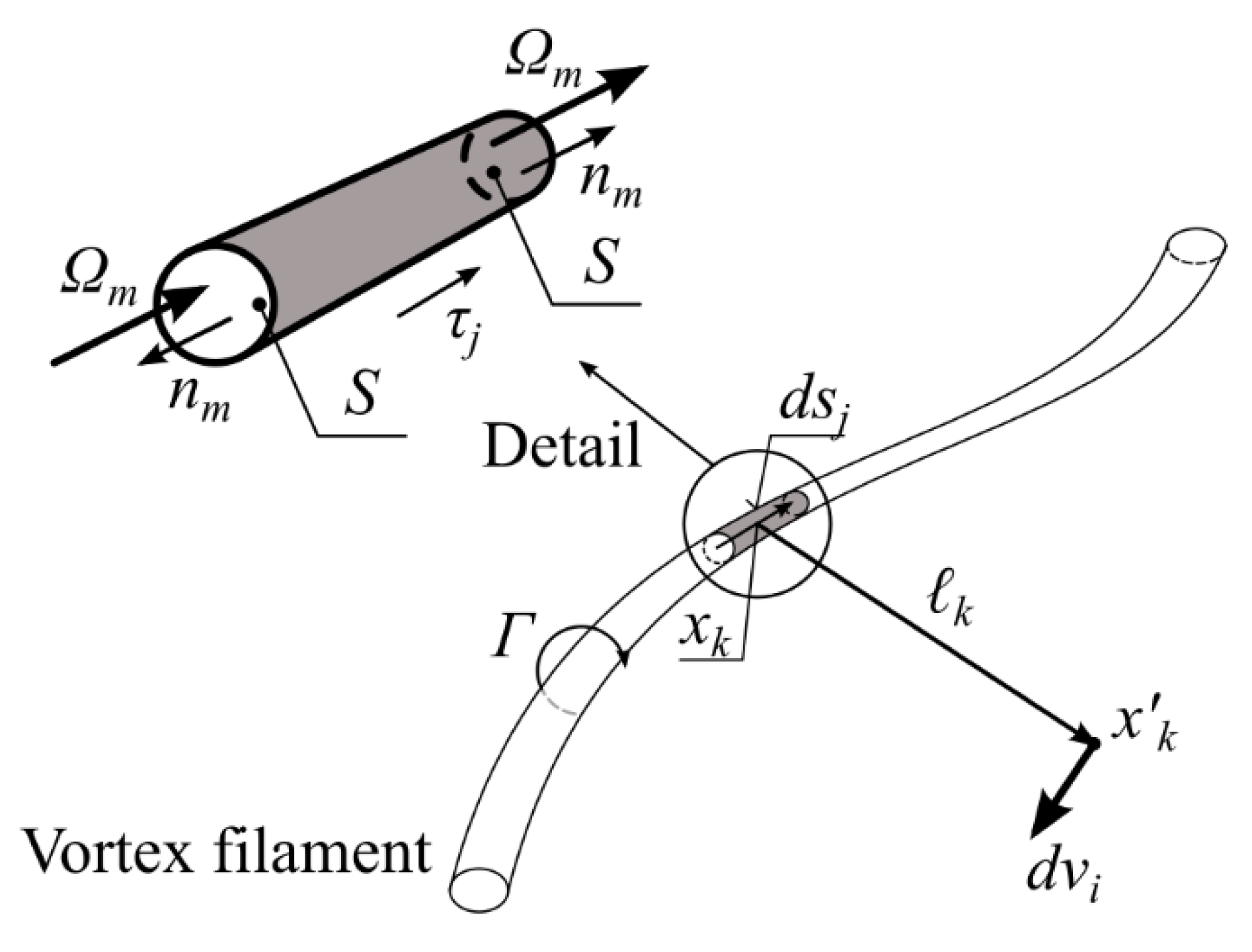
It will be useful to remind some basic terms of the vortex flow for a better understanding of the following derivations. It is possible to define vortex lines in the vorticity vector field. The vortex line is an imaginary line on which the vorticity vector is tangential at each point of it. After that, it is possible to define a vortex tube. The vortex tube is a vortex structure where the boundary is created by the vortex lines drawn through a closed curve. A vortex filament is the vortex tube with an infinitesimal area of the vortex tube cross-section. The intensity of the vortex tube/filament is defined as the flux of the vorticity vector through a cross-section of the vortex tube/filament. This flux can be expressed as a scalar product of the vorticity vector and the outward unit normal vector.
where µ is the intensity of the vortex tube/filament, nm is the outward unit normal vector to the boundary surface of the vortex tube/filament element, S is the area of the vortex tube/filament cross-section. The intensity µ of the vortex tube/filament is equal to the circulation Γ over the boundary curve of the vortex tube/filament cross-section area. This is a result of the well-known Kelvin–Stokes theorem [6].
There is a vortex filament which element dsj induces an infinitesimal velocity dvi in Figure 1. This velocity can be expressed by the Biot–Savart law applied to the vortex flow:
where Γ is the circulation around the vortex filament, r is the magnitude of the vector rk, xk is the vortex filament element location, x’k is the induced velocity location, ℓk = x’k − xk, τj is a unit vector tangential to the vortex filament. The vortex tube/filament has the same orientation as the vorticity vector Ωm.
It is possible to take into consideration the next relations:
If the element dsj is really infinitesimal, then it is possible to assume that the vectors Ωm, nm, and τj are parallel. It is possible to write:
The Biot–Savart law then becomes:
or
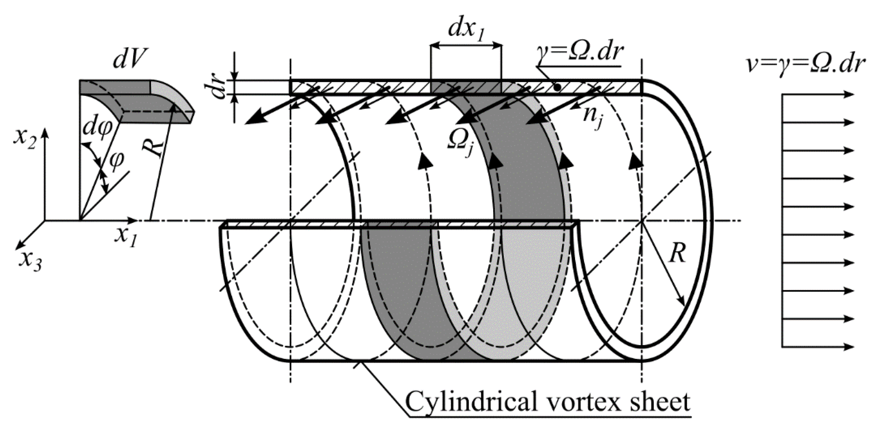
Now, it is possible to define a special vortex sheet shape in accordance with Figure 2. The shape of this vortex sheet is cylindrical. This vortex sheet consists of circular vortex filaments with radius R. The length of the cylinder is infinite. The vorticity vector magnitude is constant along the whole cylinder and the thickness of the vortex sheet is dr.
The Biot–Savart law will be applied to the infinitesimal element of this vortex sheet. Dimensions of this element are:
After applying all previous relations to (7) or (8), we obtain:
It is thus possible to introduce the linear density of vorticity γ.
If the cylindrical vortex sheet has the infinite length and the linear density of vorticity is constant over the whole vortex sheet than the infinitesimal velocity induced by the element of such vortex sheet is given by the following expression:
Equation (8) must be integrated to express the velocity induced by the whole cylindrical vortex sheet:
The tangential unit vector τj does not depend on the x1 coordinate. It is the function of the angle φ. The location of the induced velocity is given by the coordinates x’k. These coordinates are constants from the view of the integration. The coordinates xk determine the location of the vorticity element on the vortex sheet. These coordinates are variables from the point of view of the integration. Variable ℓ is the distance between xk and x’k in accordance with the Expression (5). The integral in Expression (13) has a simple analytical solution (14). This is also mentioned in [7]. The solution is:
where σi is a unit vector in the streamwise direction of the pipe axis. It means that such a circular vortex sheet induces a plug flow inside of the circular vortex sheet and no flow outside the circular vortex sheet. Another result is that this solution does not depend on the cross-section shape of the vortex sheet. The only condition is that the cross-section shape must be constant along the whole vortex sheet.
It is possible to combine two coaxial cylindrical vortex sheets now. This situation is described in Figure 3. The principle of superposition can be applied in this situation. The effects of both vortex sheets are combined. Each of the cylindrical vortex sheets influences the flow in its inside area.
Velocity for the radius interval <0, R2> is v = γ1 + γ2. Velocity for the radius interval <R2, R1> is v = γ1.
3. Basic Idea of Velocity Profile Derivation
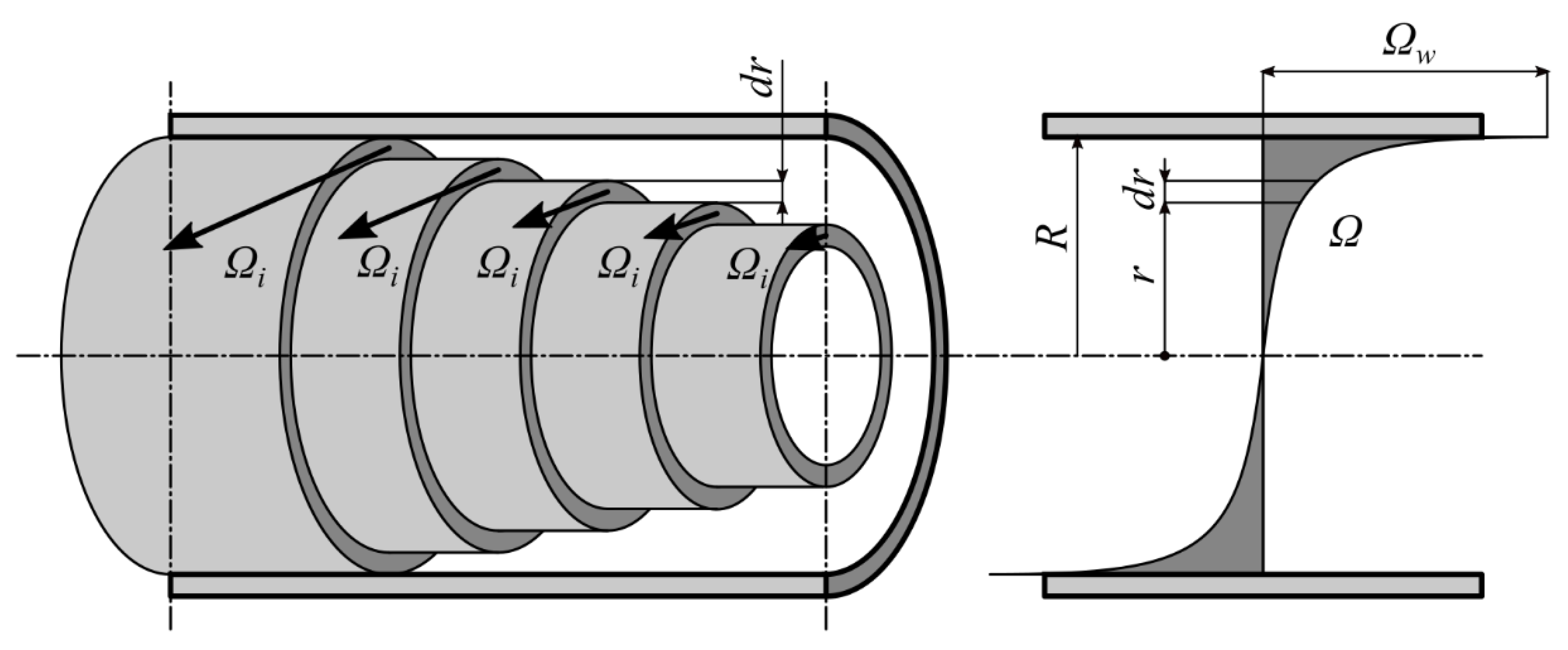
Every fluid flow is interwoven with vorticity and vortex sheets. This is also true for fluid flow in the pipes. It is possible to imagine that there are a number of circular vortex sheets inside of the pipe in accordance with Figure 4. Each of these circular vortex sheets influences the flow inside of it, but it does not influence its outside area. There are not separated vortex sheets in this case, but there is a continuous distribution of vorticity Ω over cross-section. The maximal vorticity is at the wall (Ωw).
The infinitesimal velocity induced by one circular vortex sheet with radius r can be expressed:
The vector σi is the streamwise oriented unit vector. This vector is constant over the whole domain; therefore, it is possible to neglect it for this case. The velocity magnitude will be solved only. Equation (15) will then be modified as follows:
The velocity at a given radius r* is result of the effects of the vortex sheets with radius within the interval <r*, R>. This can be expressed by the integral:
The only problem is that the function Ω is unknown for now. However, it is possible to choose a function with free coefficients which will be determined with the help of some boundary conditions. The author tested many functions, polynomial functions of different order [8], hyperbolical functions which lead to logarithmic velocity profiles, and the combination of polynomial and hyperbolical functions. Soukup [9] tested a function tangent which worked well, but it was a rather uncomfortable function to work with it. At the end, the polynomial function with four free coefficients and with two free exponents was chosen. Four free coefficients are determined from the boundary conditions. Two free exponents are determined on the basis of the absolute error minimization in comparison with the PSP experimental data.
The general form of the polynomial function can be written as:
where A(i) are the free coefficients, i is an integer in the interval <0, ∞>. The number M can be an infinite value. It means that there are an infinite number of free coefficients A(i) in the polynomial. The number of free coefficients must be restricted. The Ω function is shown in Figure 4. It is possible to assume that it is an odd function in accordance with Figure 4. It means that only the odd values of i are taken into consideration. The free coefficients A(i) represent the values of i-th derivatives of the polynomial function in the pipe axis (r = 0). The idea about using the odd polynomial function is supported by the fact that Ω = 0 for r = 0. It means that A(0) = 0. This is also the condition of smoothness of the first velocity profile derivative in the pipe axis.
The first derivative of Ω function corresponds to the second velocity profile derivative. The second velocity profile derivative in the middle of the pipe determines the curvature radius at that point. If this second derivative is zero, then the curvature radius is infinite. This is not possible. The first derivative of Ω at r = 0 cannot be zero, and it means that A(1) ≠ 0. The third derivate is also chosen not to be zero, what means that A(3) ≠ 0. The same situation is for the K-th and N-th derivatives, A(K) ≠ 0 and A(N) ≠ 0. All other derivatives in the pipe axis (free coefficients) are chosen to be zero.
The form of the chosen polynomial function is:
It is supposed that the exponent K is lower than the exponent N. The boundary conditions for the velocity or for the vorticity Ω are used to determine the four free coefficients in the polynomial.
4. Available Conditions for Free Coefficients Determining
Some information about the velocity profile and about the vorticity Ω can be used as boundary conditions. The list of all usable conditions is as follows:
- Zero velocity at the wall.
- Vorticity at the wall Ωw. This condition corresponds to the condition of pressure drop in the pipe.
- Zero value of the vorticity Ω in the pipe axis. This corresponds to the smoothness condition of the first velocity profile derivative in the pipe axis.
- The first vorticity derivative in the pipe axis. This condition corresponds to the curvature radius.
- Maximal velocity in the pipe axis.
- The knowledge of flow rate in pipe.
- The knowledge of radius where the velocity is the same as the average velocity.
- All conditions are explained in detail in the next chapters.
4.1. Zero Velocity at the Wall
This condition is fulfilled directly due to the using of the cylindrical vortex sheet. It was mentioned in the previous sections that the cylindrical vortex sheet with circular vortex lines induces zero velocity outside the cylinder and velocity v = γ inside the cylinder. It will be clearer after the velocity profile derivation.
4.2. Vorticity Value at the Wall Ωw
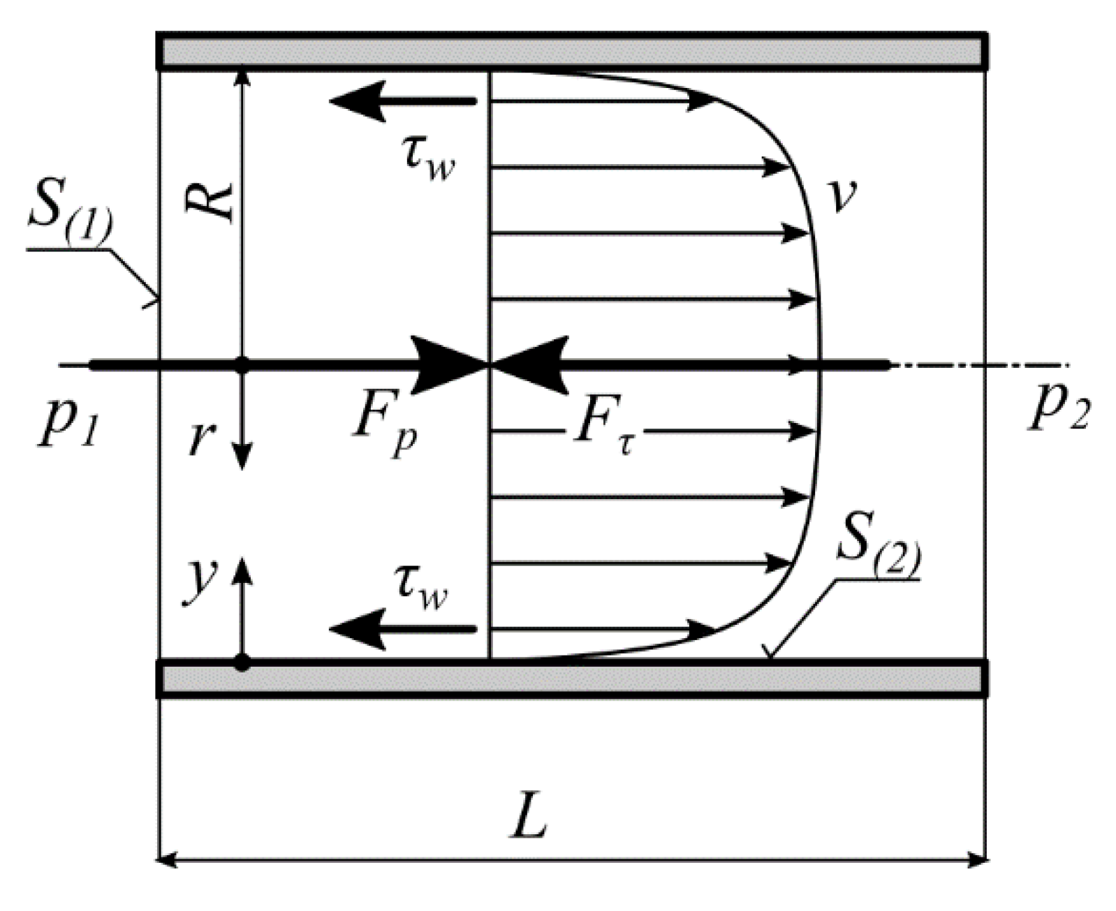
As mentioned earlier, this condition corresponds to the pressure drop condition in the pipe. The pressure drop depends on the wall shear stress τw. The pressure force Fp must be in balance with the friction force Fτ as it is depicted in Figure 5.
Pressure force can be expressed this way:
Friction force can be expressed as:
where:
The quantity η is the dynamic viscosity. Then the friction force is:
It is possible to express the value of Ωw by the force balance applying:
The pressure drop can be expressed as a function of the friction factor f. It can be expressed by using Bernoulli equation:
When the previous equation is applied into Equation (24), then we obtain:
4.3. Zero Value of the Vorticity Ω in the Pipe Axis
If the vorticity Ω is zero for r = 0, then it means that the first velocity profile derivative is also zero. It is apparent from relation (2). This condition ensures the smoothness of the velocity profile in the pipe axis. Some models of the mean velocity profiles for turbulent flow have a problem with this condition [1,2].
4.4. The First Derivative of the Vorticity Function Ω in the Pipe Axis
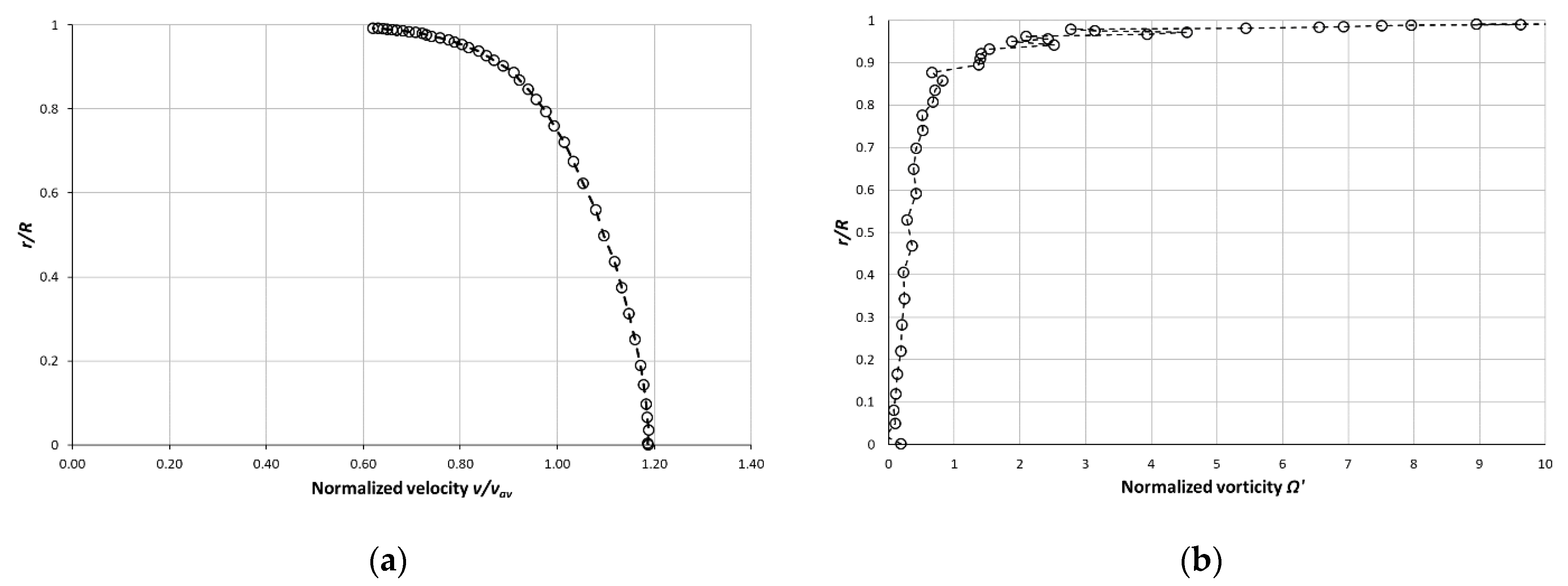
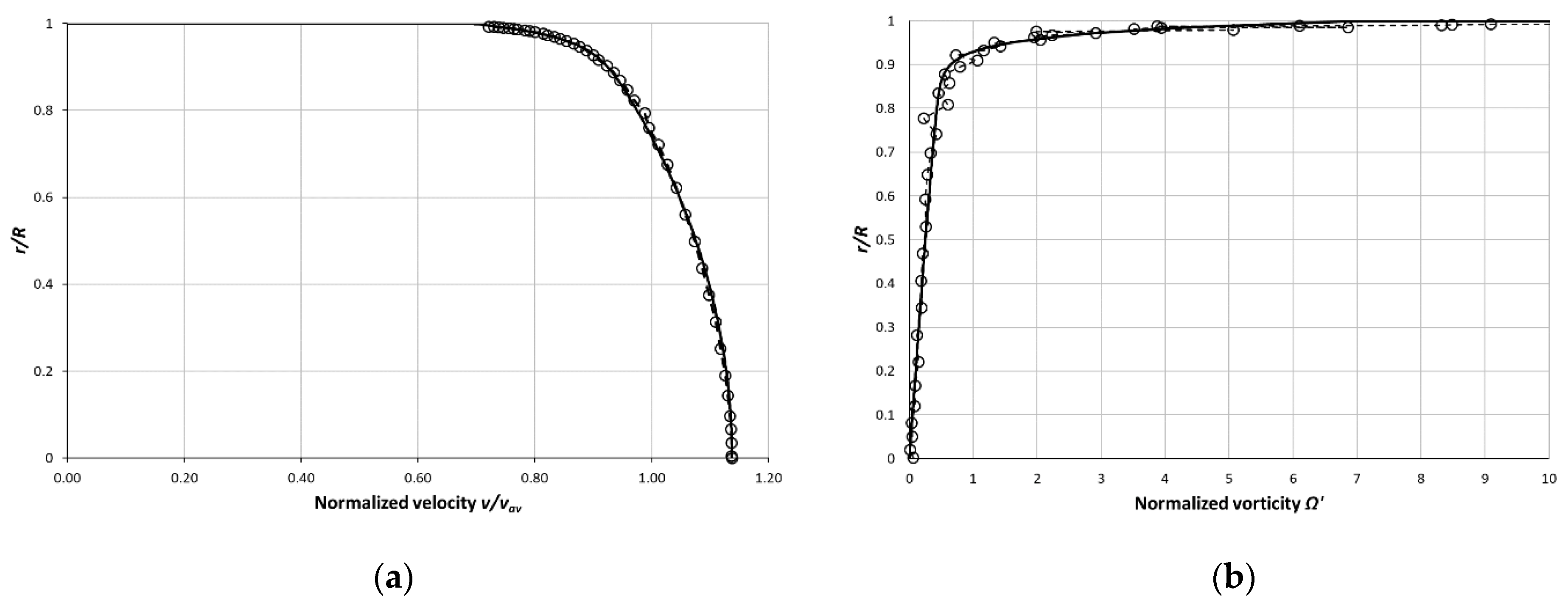
This condition is new and essential. The first derivative of Ω corresponds to the second velocity profile derivative. They differ by sign only. It follows from Expression (2). The values of vorticity Ω can be calculated from the mean velocity profiles. The value of Ω is calculated from the mean velocity profile acquired experimentally (PSP), for Reynolds number 230,460 is in Figure 6.
The results for other values of Re are similar like in Figure 6. The vorticity distribution is rather bumpy even though the mean velocity profile looks smooth. The vorticity distribution is close to the linear function near the pipe axis. It means that the vorticity derivative is constant within that area. This leads to the deduction that the curvature radius of the mean velocity profile is constant, and the velocity profile is nearly parabolic in this area. It is possible to find the value of the vorticity derivative by a linear substitution of the vorticity distribution calculated from the measured mean vorticity profile. The question is how it depends on Re or on the other quantity? It was found, by analysis of PSP data, that there is a problem in the dependence on Re. The Reynolds number was increased by increasing of the density/pressure of the air in case of PSP measurements. This causes the problem with the finding of the vorticity derivative dependence on the Re. It will be explained later. Now it will be useful to express the second mean velocity profile derivative for laminar flow. The velocity profile for laminar flow can be expressed by the next formula.
The first velocity derivative is:
The second velocity derivative (negative first vorticity derivative) is:
The second mean velocity profile derivative is marked by subscript 1 because it is also the negative first vorticity derivative.
When the normalized velocity profile for the laminar flow is taken into consideration, then the velocity profile will have the following form:
where v’ is a velocity normalized by the average velocity v(av) and r’ is a radius normalized by the pipe radius R, r’ = r/R. Then, the first normalized velocity derivative has the following form:
The second normalized velocity derivative is:
The second normalized velocity derivative (negative first normalized vorticity derivative) is constant in the case of the laminar flow.
It is clear from Equation (29) that the second velocity derivative or the first vorticity derivative for the laminar flow depends on the average velocity and on the pipe radius. In the case of the normalized velocity profile, it is a constant value.
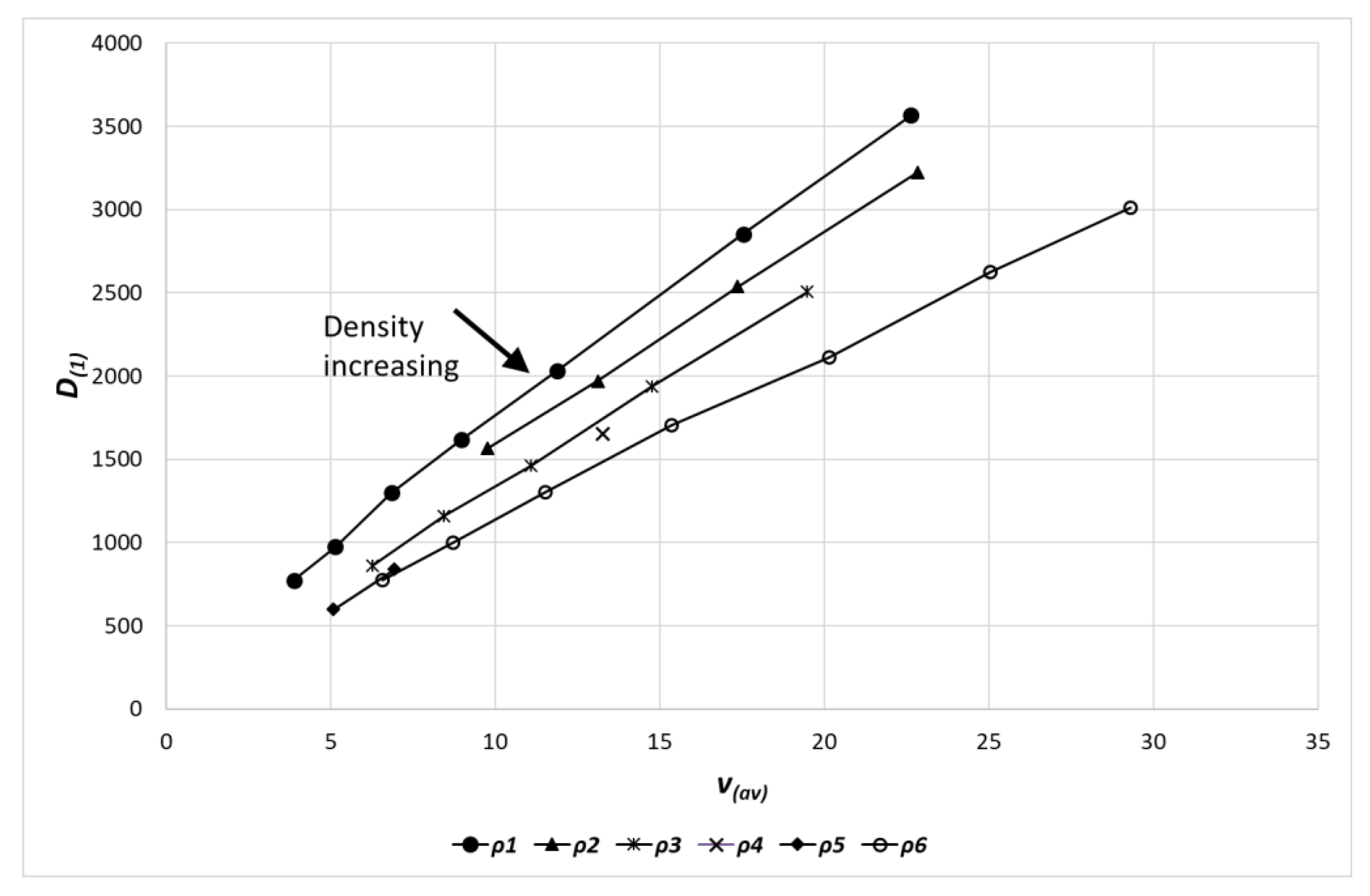
As mentioned earlier, it was found that the first vorticity derivative at the pipe axis, in the case of turbulent flow, depends linearly on the average velocity under the condition that the air density is constant. If the density is changed, then the linear dependence is different. These dependences are drawn in Figure 7.
This condition should be researched in detail in future. This condition will be discussed later in this paper.
4.5. Maximal Velocity in the Pipe Axis
The maximal velocity is possible to use as a condition because it depends on Re. It means that we take it as a known quantity. This is described in detail in [8]. The difference between v(max) and v(av) can be normalized by the average velocity. This way, we obtain a value which is signed as n.
Then:
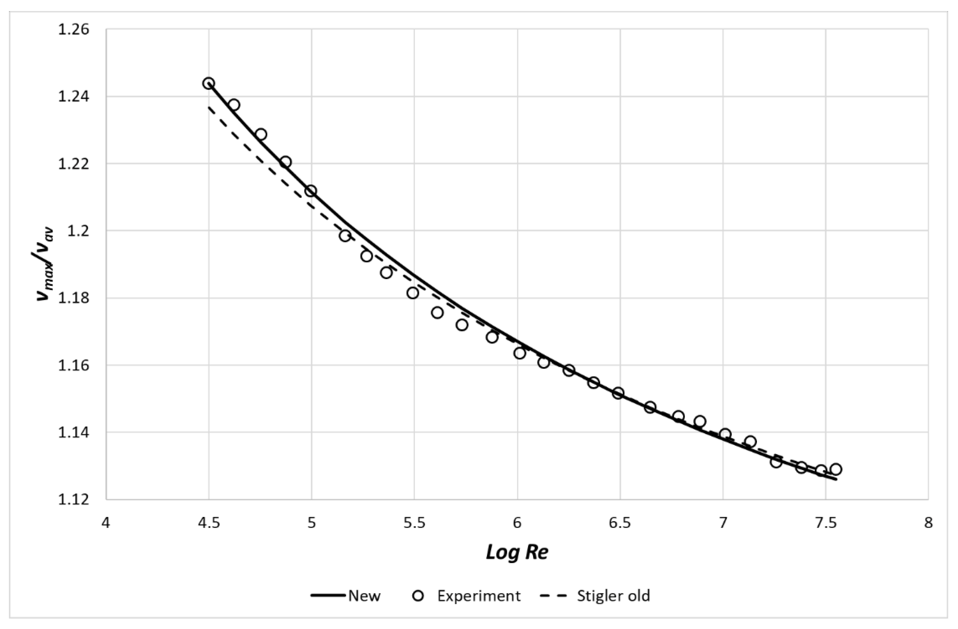
The normalized maximal velocity as a function of Re is shown in Figure 8.
The number n depends on the Re. For laminar flow is n = 1 and it decreases with the Re increasing. The dependence of n on Re, for the range Re = <31,577; 35,259,000> can be expressed this way [8]:
The constants are A = 1.789 and B = −1.392 in literature [8]. This dependence is represented by the dashed line in Figure 8. Here it was found that the better values are A = 1.8902 and B = −2.0373. This dependence is represented by the solid line in Figure 8. The empty circle symbols represent experimental data (PSP). On the basis of Expressions (34) and (35) it is possible to write
The approximation of the normalized maximal velocity is rather good. However, it would be better to do more experiments to improve Expression (36).
4.6. The Knowledge of Flow Rate in Pipe
This is an essential and elementary condition. If we know the mean velocity profile, then it is possible to express this condition this way
where Q [m3.s−1] is the flow rate, S is the cross-section area. If the cross-section has a circular shape, then the infinitesimal area dS can be expressed as:
The radius r is the only variable. The flow rate can be then expressed by the finite integral:
The only problem is to find a function for the velocity v which will be possible to integrate. If we know the average velocity, then the flow rate can be also expressed this way:
4.7. The Radius of the Average Velocity
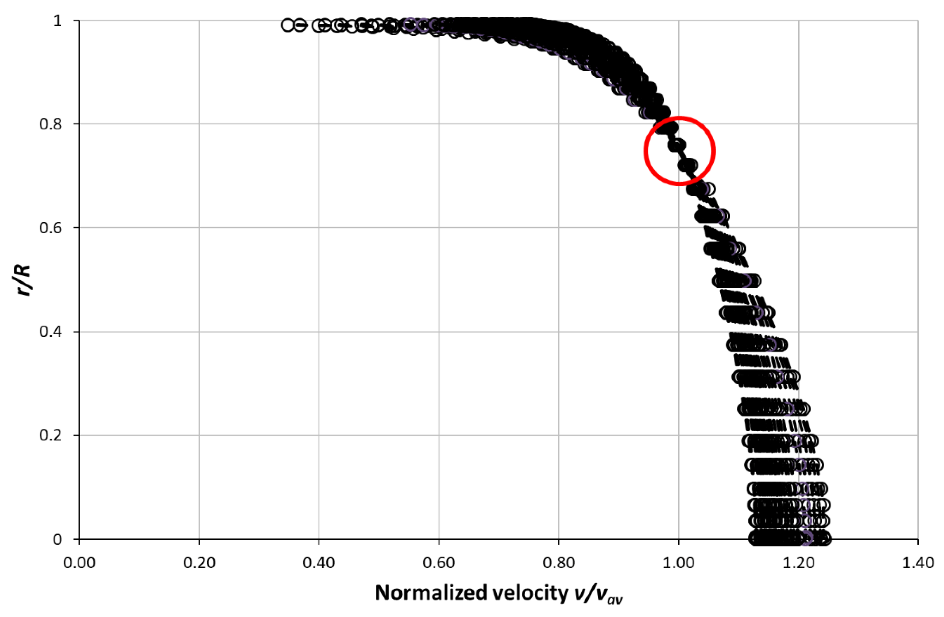
This is the last condition for now. When we draw all 26 mean velocity profiles measured by Zagarola [3] (PSP) and when we normalize them by the average velocity, as shown in Figure 9, then it is apparent that all of them are crossing at one point with the normalized velocity with value 1.
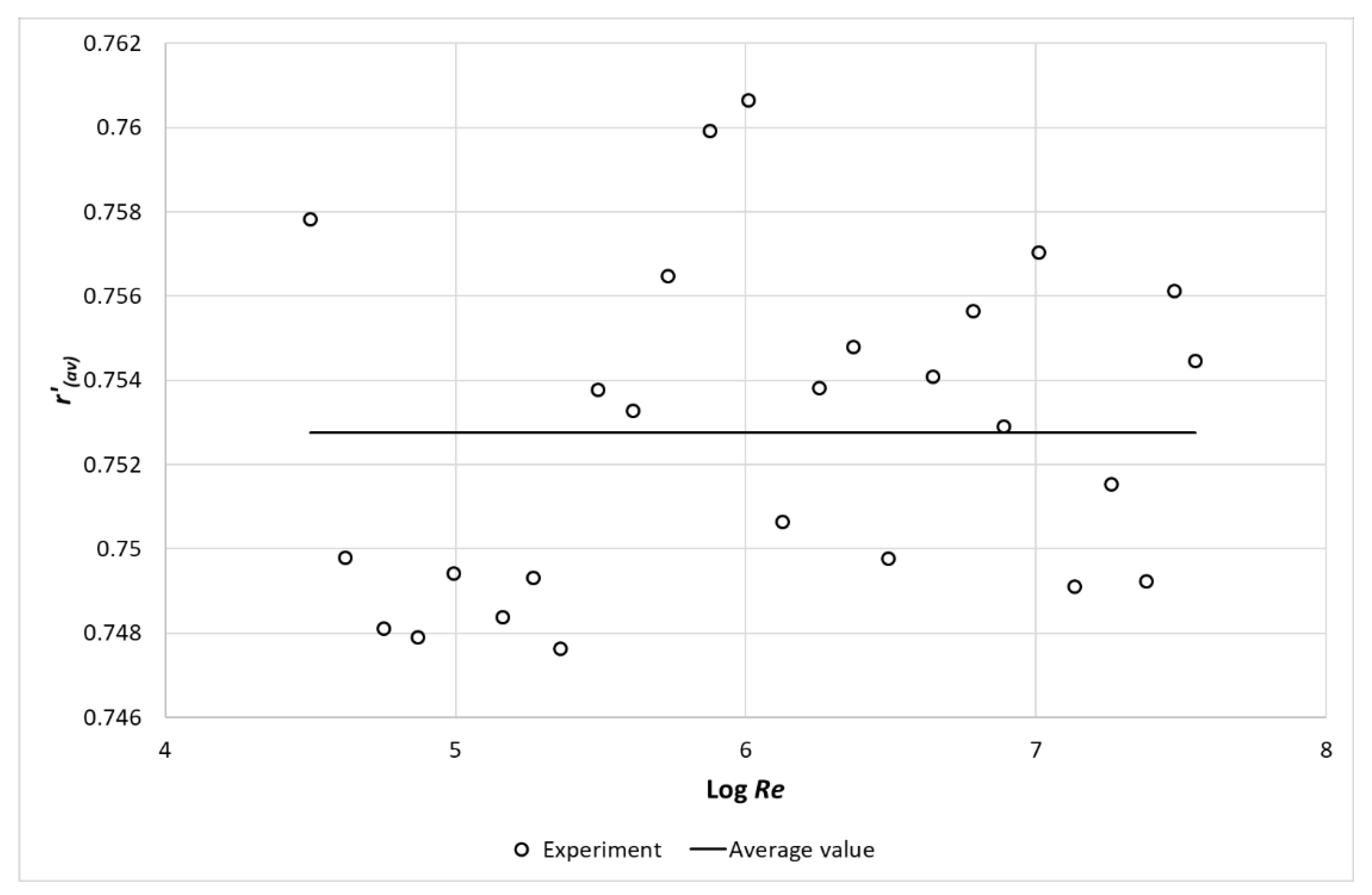
The normalized radius for the average velocity for all profiles is possible to determine in a numerical way. The values of average velocity radius for all profiles are in Figure 10.
It is possible to see that the values tend to oscillate around a constant value for a given Re range. The average velocity radius range is <0.74763; 0.76064>. The range width is 0.013012, which is 1.3% of the total normalized radius range. The average value of the average velocity radius is 0.75275. It is necessary to carry out more measurements to prove this result. This condition was not used during the mean velocity profile derivation.
5. Mean Velocity Profile Formula Derivation
The derivation of the analytical formula of the mean velocity profile is based on the Expressions (17) and (19). When we put together these equations, then we obtain:
where the low integral radius limit r* is the radius where we want to know the mean velocity because the velocity is influenced only by the vorticity outside the radius r*. The analytical solution of this integral is rather simple.
Hereinafter, the variable r* will be replaced by r. The Expression (42) will take the following form:
The boundary conditions are applied to find four free coefficients A(1), A(3), A(K), and A(N). The condition of the first vorticity derivative, or the negative value of the second velocity derivative in the pipe axis can be expressed this way:
where D(1) is the value of the first vorticity derivative. This value depends on Reynolds number. This dependence will be discussed later. Next condition is the vorticity value on the wall. It means the value of vorticity for r = R. The expression of this condition has the following form:
where Ωw is derived from the pressure drop. The third condition is the condition of the maximal velocity in the pipe axis. It is derived from the Expression (43) for the case that r = 0.
The last condition is the condition of the flow rate. It is possible to obtain this condition by applying of expression for velocity (43) and flow rate (40) into the expression for flow rate (39). After that it is possible to obtain this condition in the next form:
As mentioned above, there are three unknown free coefficients. There are also three Equations (45)–(47). It is possible to solve them and express all free coefficients. Expression for each coefficient is:
where:
It is possible to introduce the next parameters:
The formula for the velocity profile (43) will then be:
The normalized mean velocity profile for comparison of different profiles will be introduced now. The radius is normalized by the pipe radius R and the velocity is normalized by the average velocity v(av)
The normalized mean velocity profile is:
The first and the second derivatives of the normalized velocity profile will be derived now:
When the relations (54) are introduced, then we obtain:
The expression closed in the square bracket is the vorticity function Ω with respect to (19). Thus, it is possible to write:
The normalized vorticity on the wall as a function of the friction factor f (26) can be then expressed this way:
Now it is possible to continue with the second normalized mean velocity derivative (the first vorticity derivative). Similar way as in the case of the first derivative, it is obtained:
Expression (62) shows the relationship between the first normalized vorticity derivative and the first vorticity derivative. When the first vorticity derivative in the pipe axis is signed as D(1) (D′(1)), Expression (62) becomes:
At the end, the only problem is to determine the exponents K and N. They can be determined by two different ways. The first one determines the exponents by minimization of the absolute difference sum between the analytical velocity profile and the experimentally obtained values. This way is used here in this paper. Another way is to find the values of exponents K and N with help of the unused boundary condition. In this case, it can be the condition of the average velocity radius.
6. Exponents Determination
As mentioned earlier, the exponents K and N are determined by the minimization of the sum of the velocity magnitude difference. The difference means the difference between the analytical profile and the experimental data. All parameters necessary to determine the analytical velocity profile (v(av), v(max), Ω(w), D(1)) are listed in Table 1. They are listed for all PSP velocity profiles. The variables, which enter into the minimization process, are exponents N and K in this case. They are highlighted in grey in Table 1.
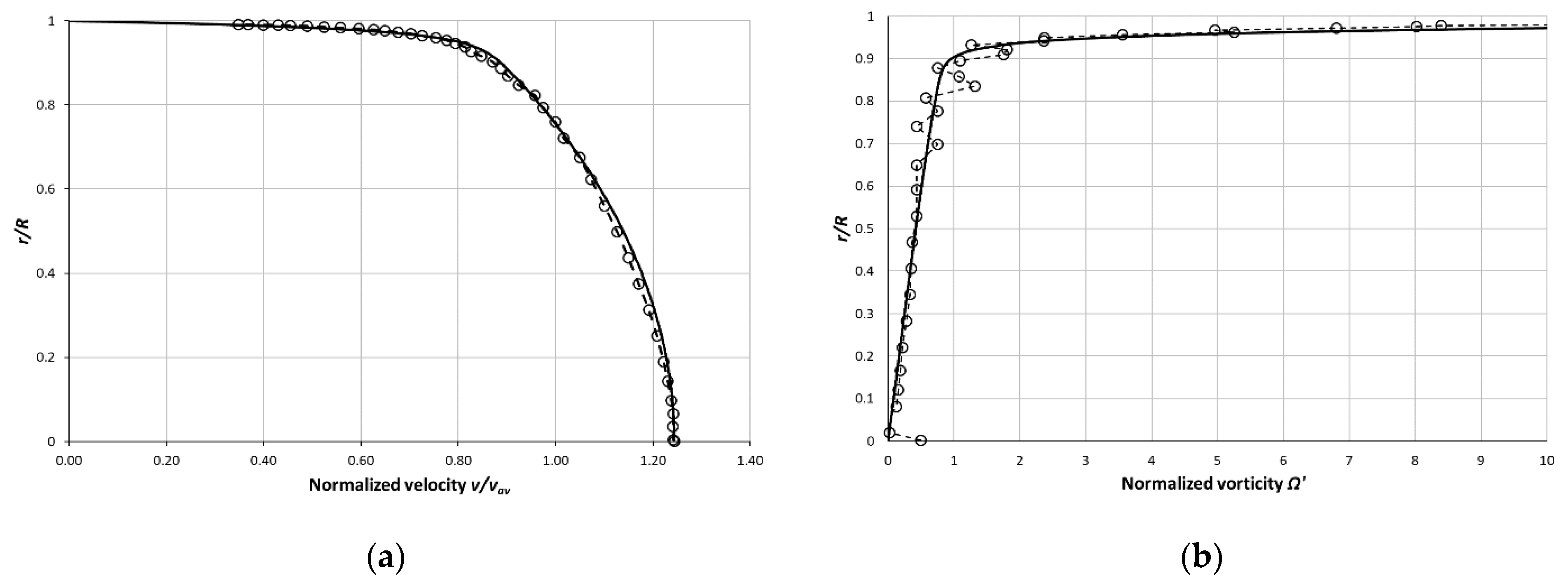
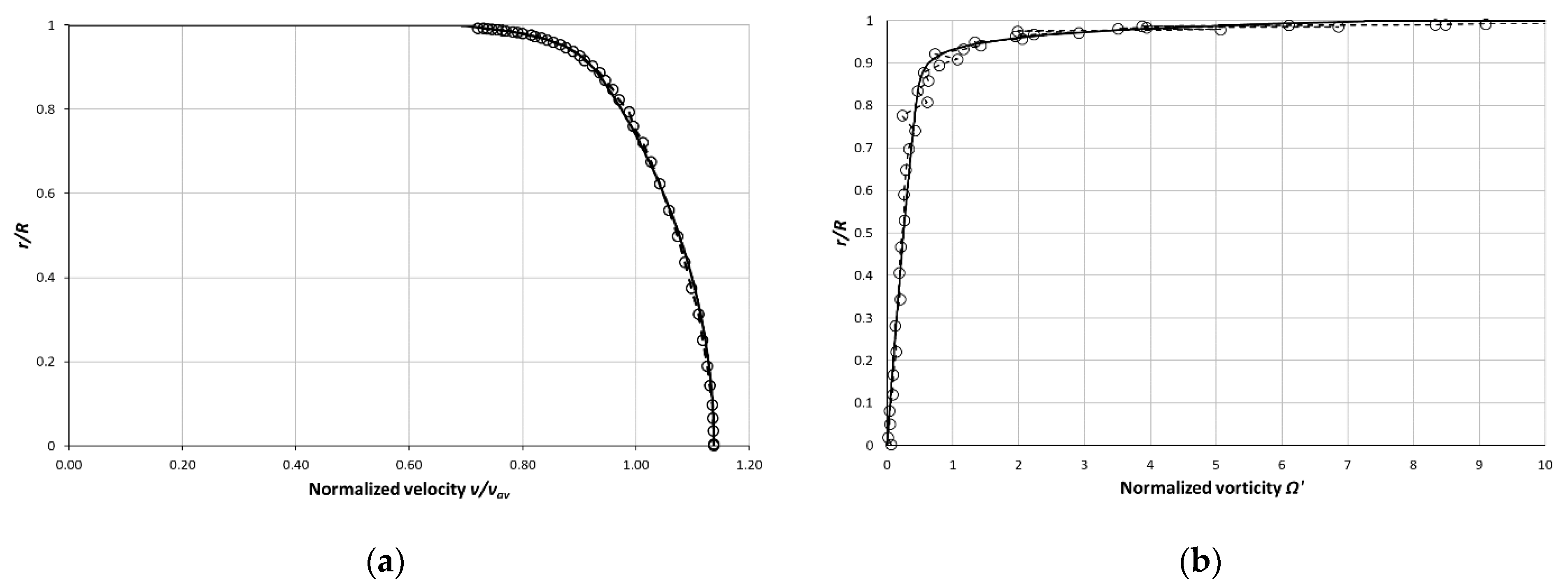
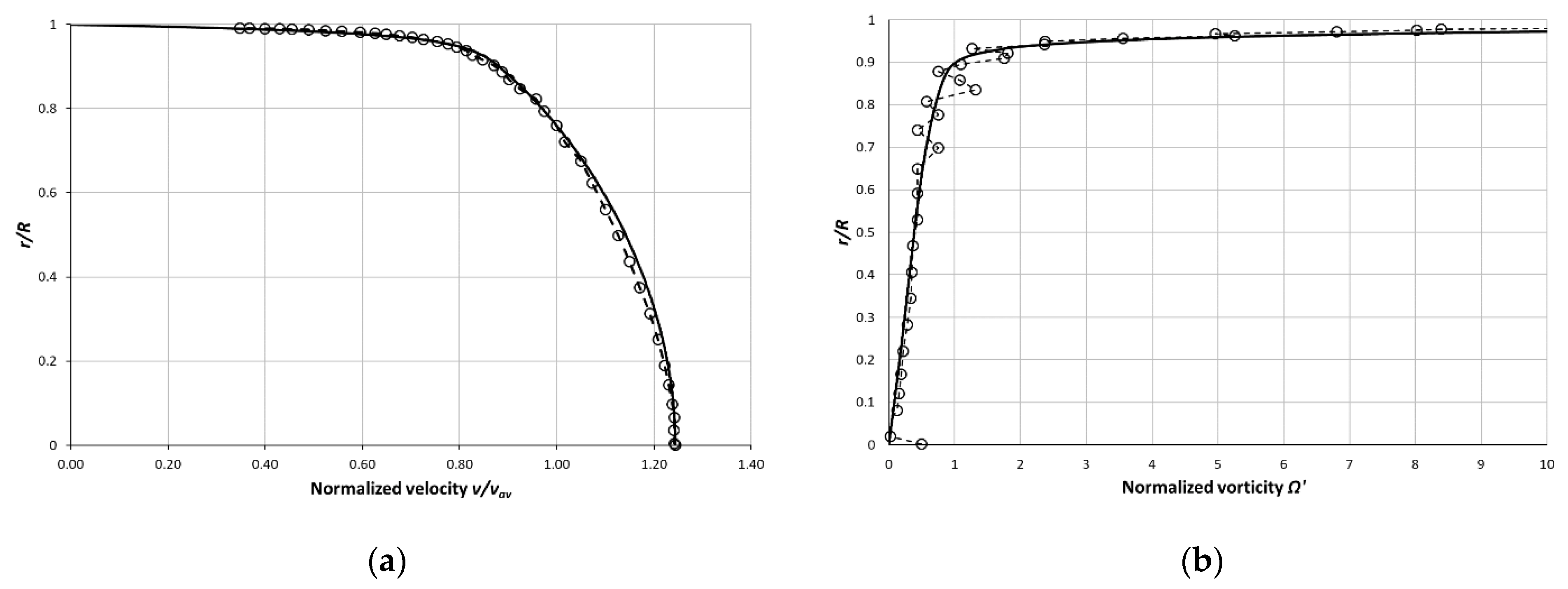
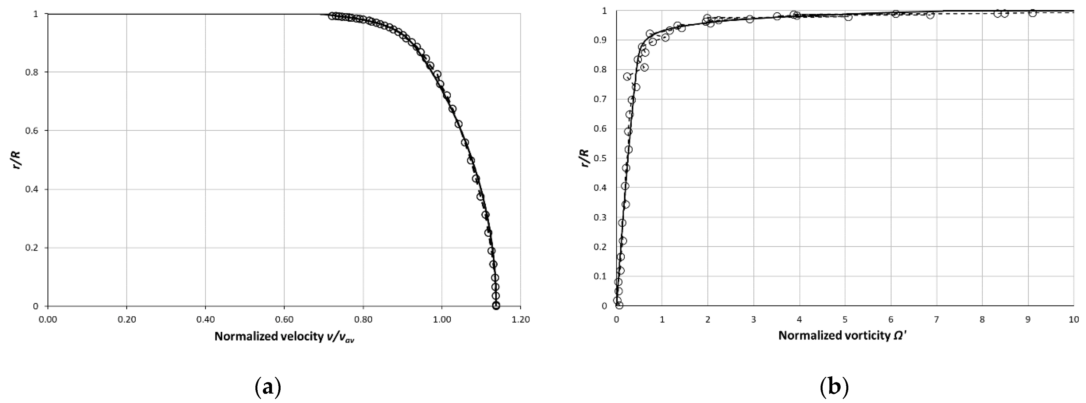
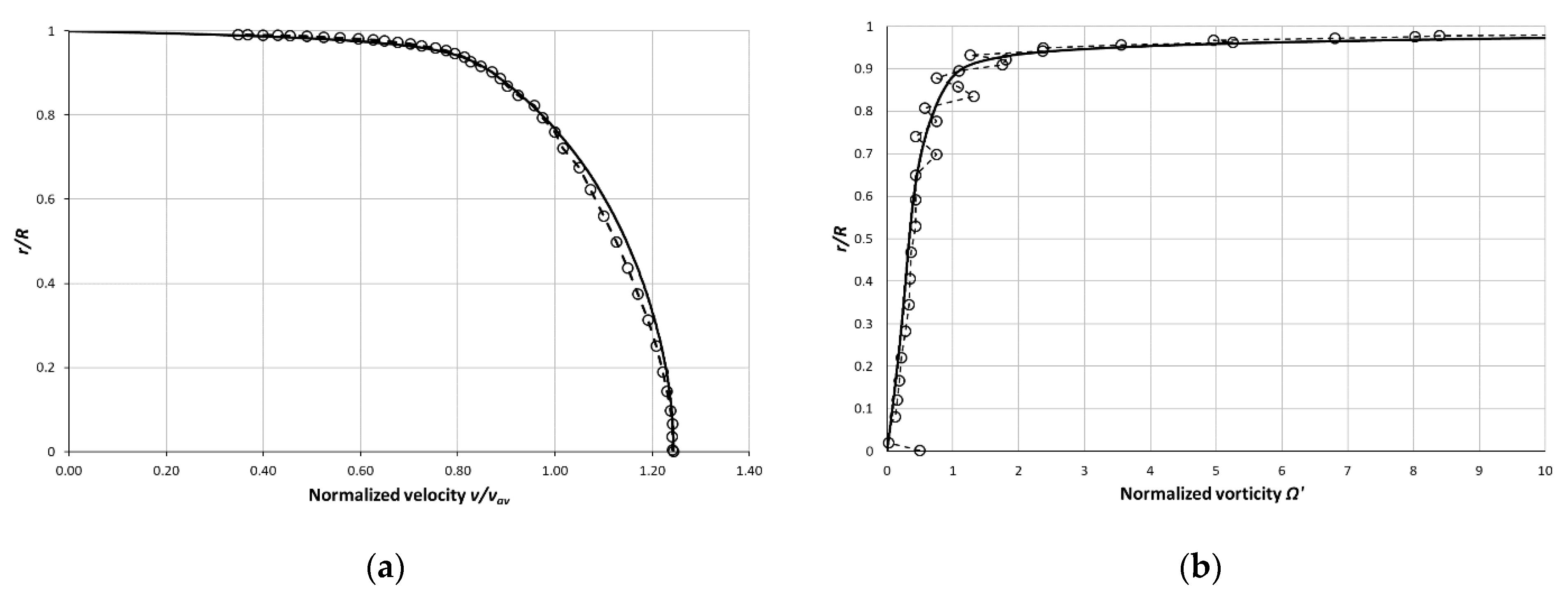
The values of v(av), v(max) are taken directly from the experimental data. The vorticity at the wall Ω(w) is calculated from the pressure drop through Expression (24) or (26). The normalized vorticity at the wall is expressed by (60). First, the vorticity derivative at the pipe axis is taken from the vorticity distribution calculated from the experimental data. The vorticity distribution near the pipe axis was approximated by a linear function from which the first vorticity derivative was calculated. The comparisons of the analytical velocity profiles and the experimental data are in Figure 11 and Figure 12. Figure 11 shows the results for the low Re. Results for the high Re are shown in Figure 12.
The average absolute difference percentage, related to the average velocity, is used for analytical velocity accuracy evaluation. It is signed as δ and its definition is in Expression (64):
where v(exp) is the experimental velocity at a given radius r, v(an) is the analytical velocity at a given radius r, v(av) is the average velocity, M is the number of measured velocities, v’(exp) is the normalized experimental velocity at a given radius r, and v(an) is the normalized analytical velocity at a given radius r. The value of s for the case of low Re (31,577) is s = 2.183 and for the case of high Re (13,598,000) is s = 0.364.
It is obvious that the velocity profiles fit better in the case of higher Reynolds numbers. There is a question about the basic parameter measurement precision as well as the mean velocity measurement precision. For example, the vorticity at the wall Ω(w) plays a crucial role in the accuracy of the analytical velocity profile, therefore the precise pressure drop measurement is essential. The problems with the mean velocity measurement are apparent from the vorticity diagram. The vorticity values calculated from the experimental data are very scattered. It is clear from Figure 11b and Figure 12b.
It is possible to test the vorticity values at the wall by the variables number extension which enter to the minimization process. The vorticity at the wall Ω(w) and the first vorticity derivative in the pipe axis D(1), as a new variable, are added to the exponents K and N. Table 2 shows the parameters obtained, for this case, by the velocity difference absolute value minimization. The grey columns emphasize the parameters which are taken as a variable in the minimization process.
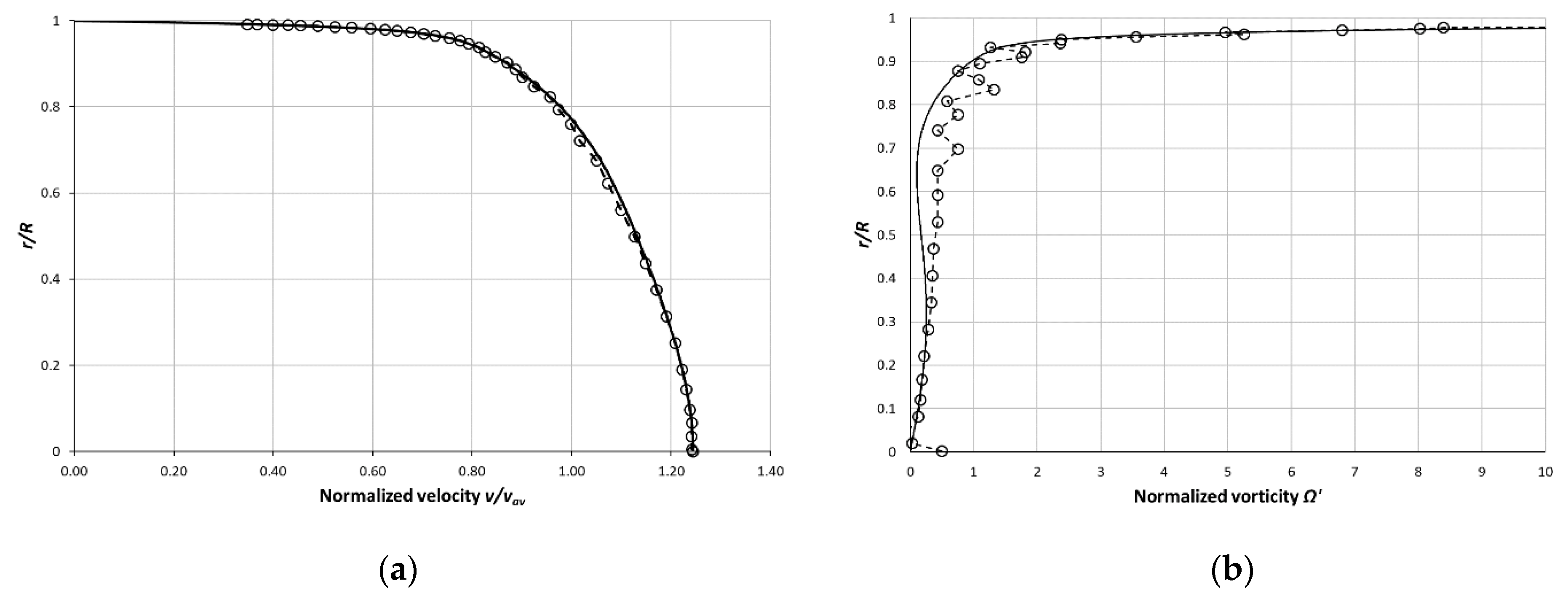
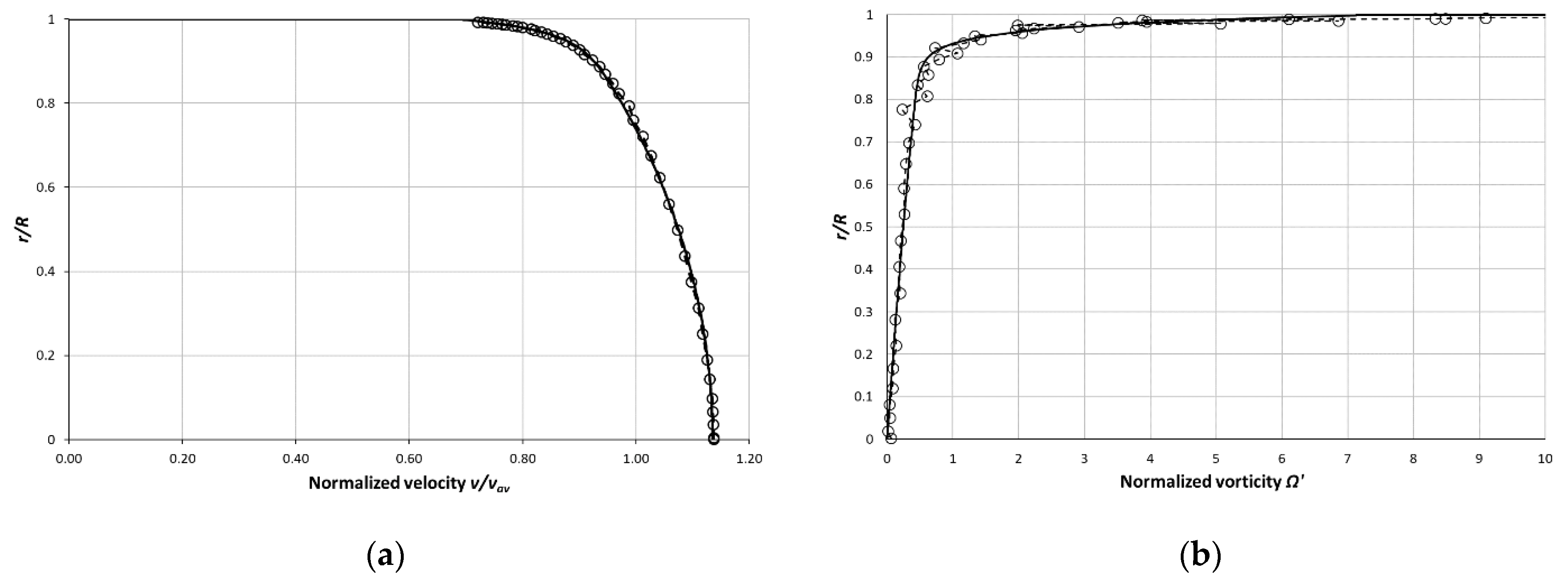
The velocity profiles for the same Re as in Figure 11 and Figure 12 are drawn in Figure 13 and Figure 14. When we compare Figure 12 and Figure 14 for high Re, then the improvement is not so apparent. The different situation is in the case of low Re. When we compare Figure 11 and Figure 13, then it is obvious that the analytical velocity profile for four variables fits better than the analytical velocity profile for two variables which are entering into the optimization. The analytical mean velocity profile precision can be evaluated by the average absolute difference percentage s (64). The s for the low Re (31,577) is s = 0.494 and for the high Re (13,598,000) is s = 0.362 in this case. The improvement of the curve fit is very high in case of low Re, but in case of high Re it is negligible.
However, the vorticity distribution is rather unusual in the case of four variables and low Re. The inflex point appears in this case. The vorticity is near to be negative in some radius range. This is something unexpectable in the case of mean velocity profiles. The question is: Where is the mistake? Are there some bumps upstream in the pipe? Is it the problem of velocity profile measurement?
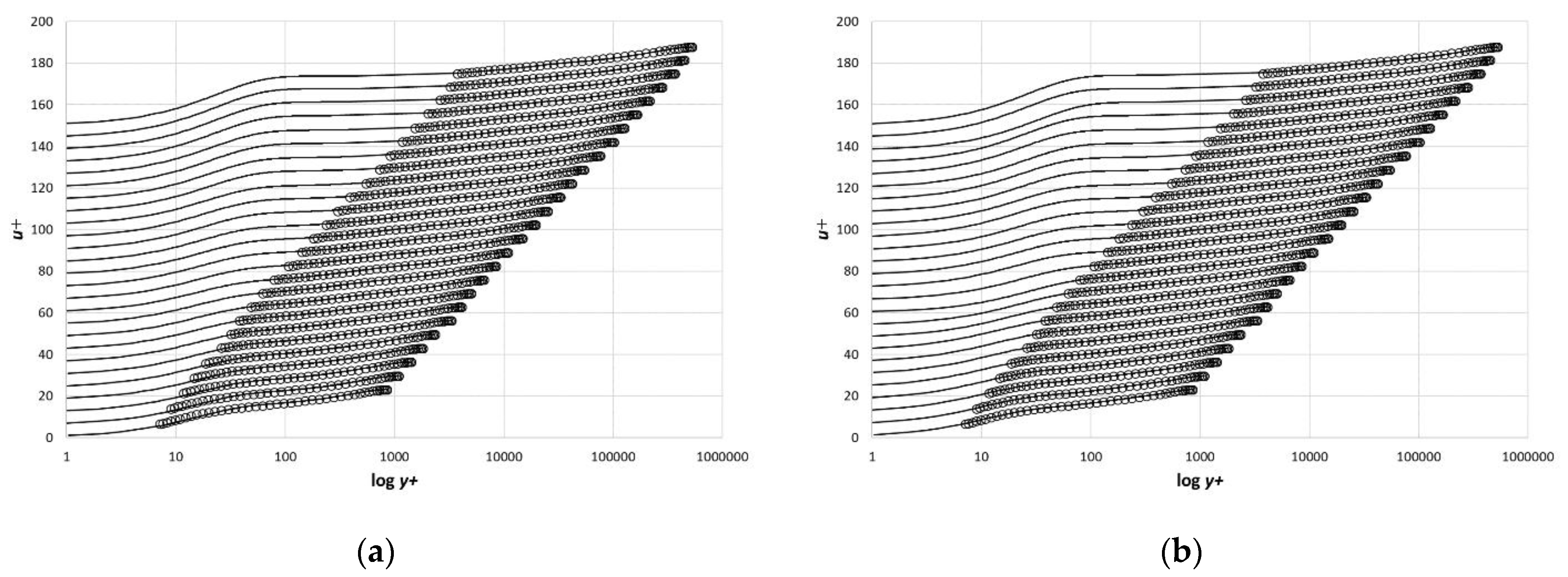
It is also possible to compare the velocity profiles in coordinates u+ and y+. The definition of u+ is in (64) and the definition of y+ is in (65).
where v is the velocity, uτ is the friction velocity, τw is the wall shear stress, ρ is the density, and ν is the kinematic viscosity. All velocity profiles in coordinates u+, y+, for the case of two variables N and K are drawn in Figure 15a. Each of the profiles is shifted about u+ = 6 from the previous one. The solid lines represent the analytical velocity profiles, and the circles represent experimental data.
The analytical profiles do not fit well in the case of low Re velocity profile. This is in accordance with our previous outcome.
The velocity profiles in coordinates u+, y+ for the case of four variables Ω(w), D(1), N, and K are drawn in Figure 15b. It is apparent that the analytical velocity profiles for low Re fit much better with the experimental data than in the previous case.
The analytical velocity profiles are very sensitive to the wall vorticity Ω(w). It is possible to compare the wall vorticity for the cases of two and four variables which are coming into the optimization process. The wall vorticity in the case of two variables is taken from the pressure drop obtained by the experiment. In the case of four variables, the wall vorticity is one of the variables which are obtained by the velocity difference minimization. It is better to compare the normalized wall vorticity which is expressed by Expression (60). The comparison is in Figure 16.
It seems, from Figure 16, that the wall vorticity is underestimated in the case of experimental data for low Re. The agreement is rather good for high Re, but the experimental values are slightly over estimated. Despite of it, the wall vorticity is more consistent in the case of the values from experiment. It is necessary to be cautious to give the exact judgement of what is correct and what is wrong because the velocity profiles are influenced by all parameters’ measurement precision. No one knows if the problem is in the measurement precision of the pressure or the mean velocity.
The next question is whether it is possible to find an analytical dependence of D(1), N, and K on Re to be able to predict the velocity profile without actual experimental data.
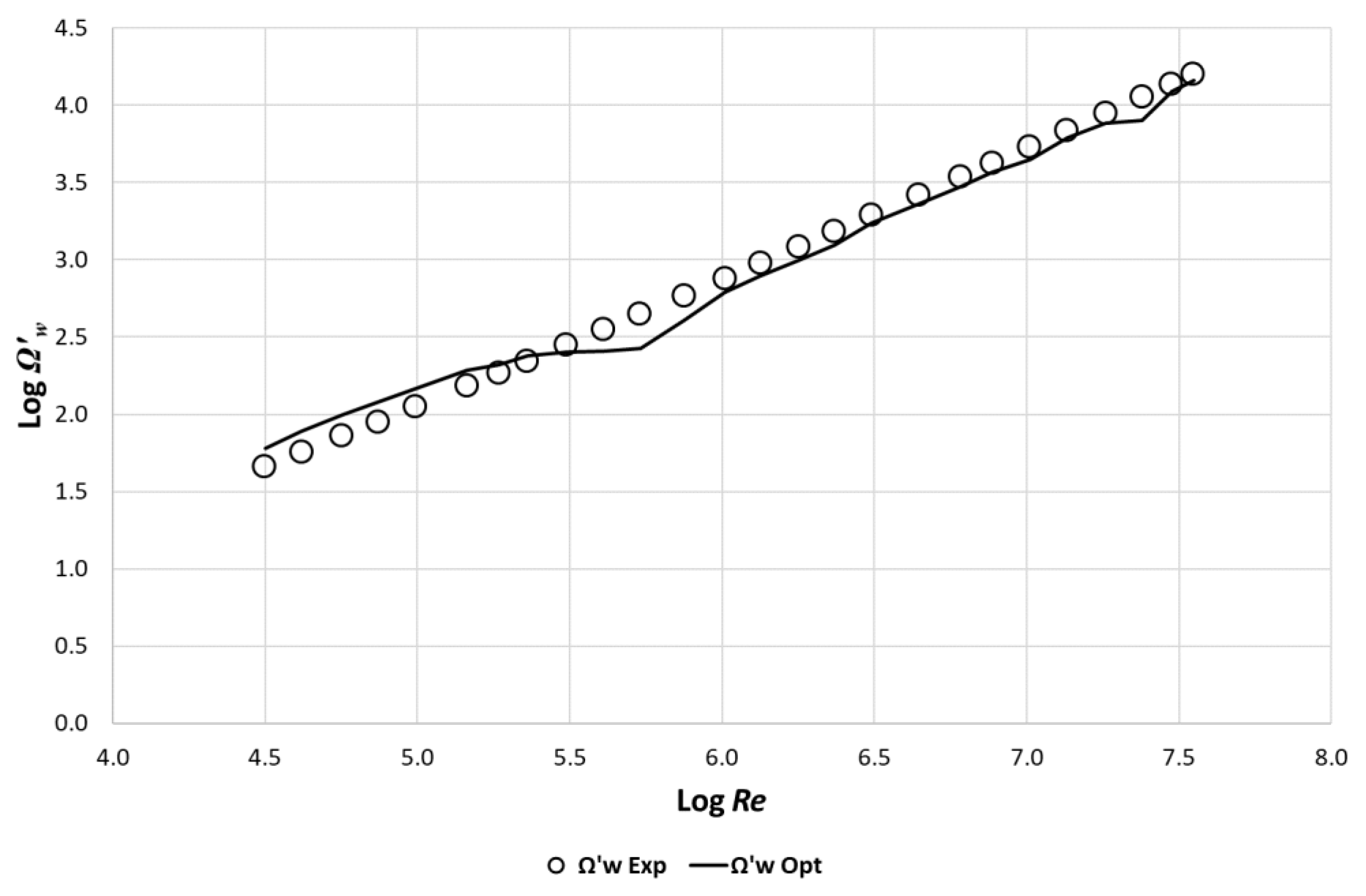
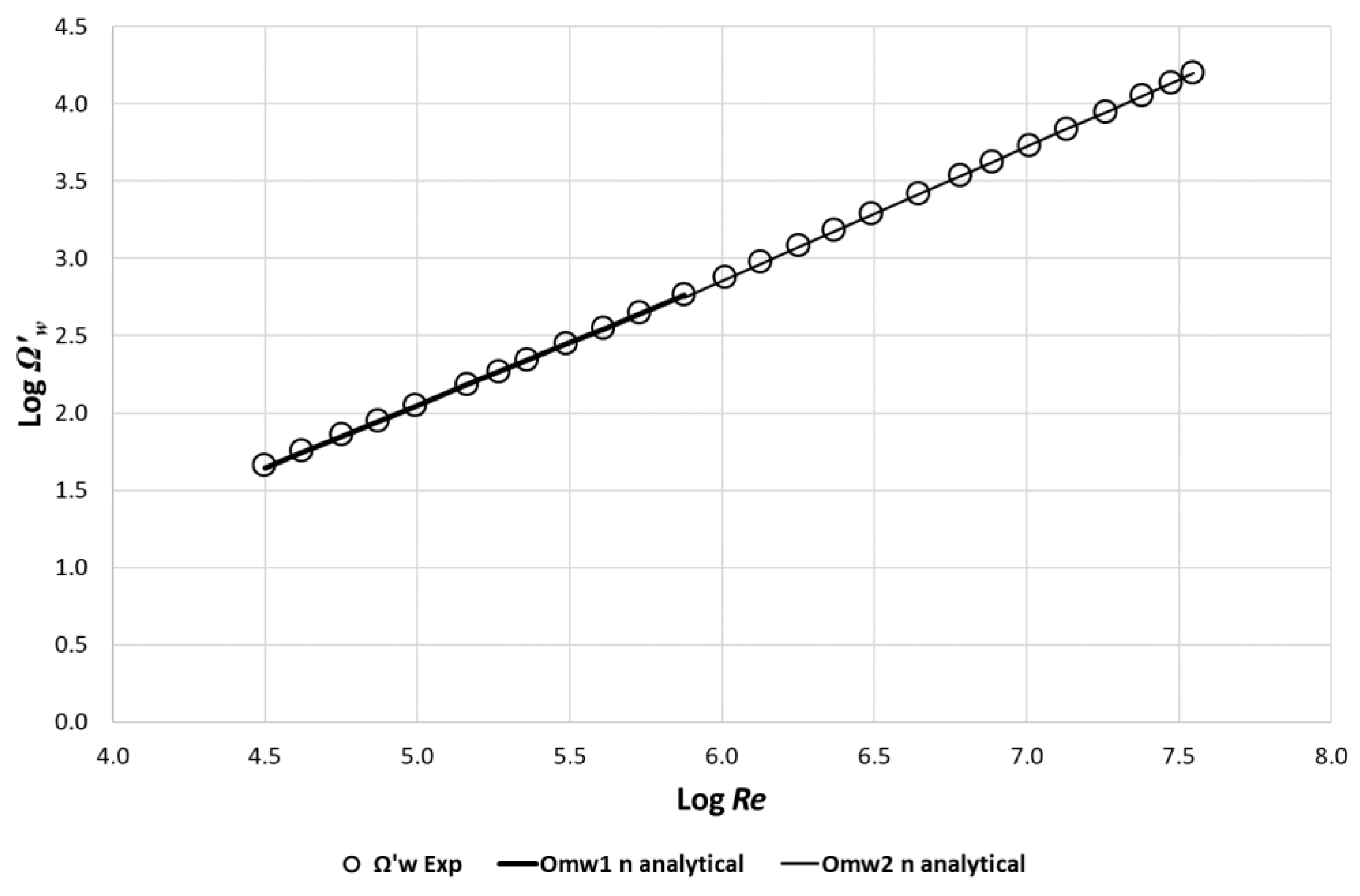
7. Normalized Wall Vorticity Ω′(w) as a Function of Re
First, attention will be focused on the normalized wall vorticity Ω′(w). Even though the normalized wall vorticity can be expressed with the help of the friction factor, it will be useful to find an expression for the dependence of Ω′(w) on the Re. The interval of Re will be divided into two parts. The functions will be defined separately for each interval. The general form of the function is:
The constants A(Ωw) and B(Ωw) depend on the interval of Re. For the interval Re < 31,500, 550,000>, the constants are A(Ωw) = 0.810279 and B(Ωw) = 100.1872, and for the interval Re <550,000, 35,259,000>, the constants are A(Ωw) = 0.868399 and B(Ωw) = 227.1003. These constants are derived on the basis of the comparison of these functions with the experimental data of (PSP) [3]. The comparison of the empirical expression and data from the experiment is in Figure 17. The agreement seems to be good.
8. The Dependence of the First Vorticity Derivative at the Pipe Axis on Re
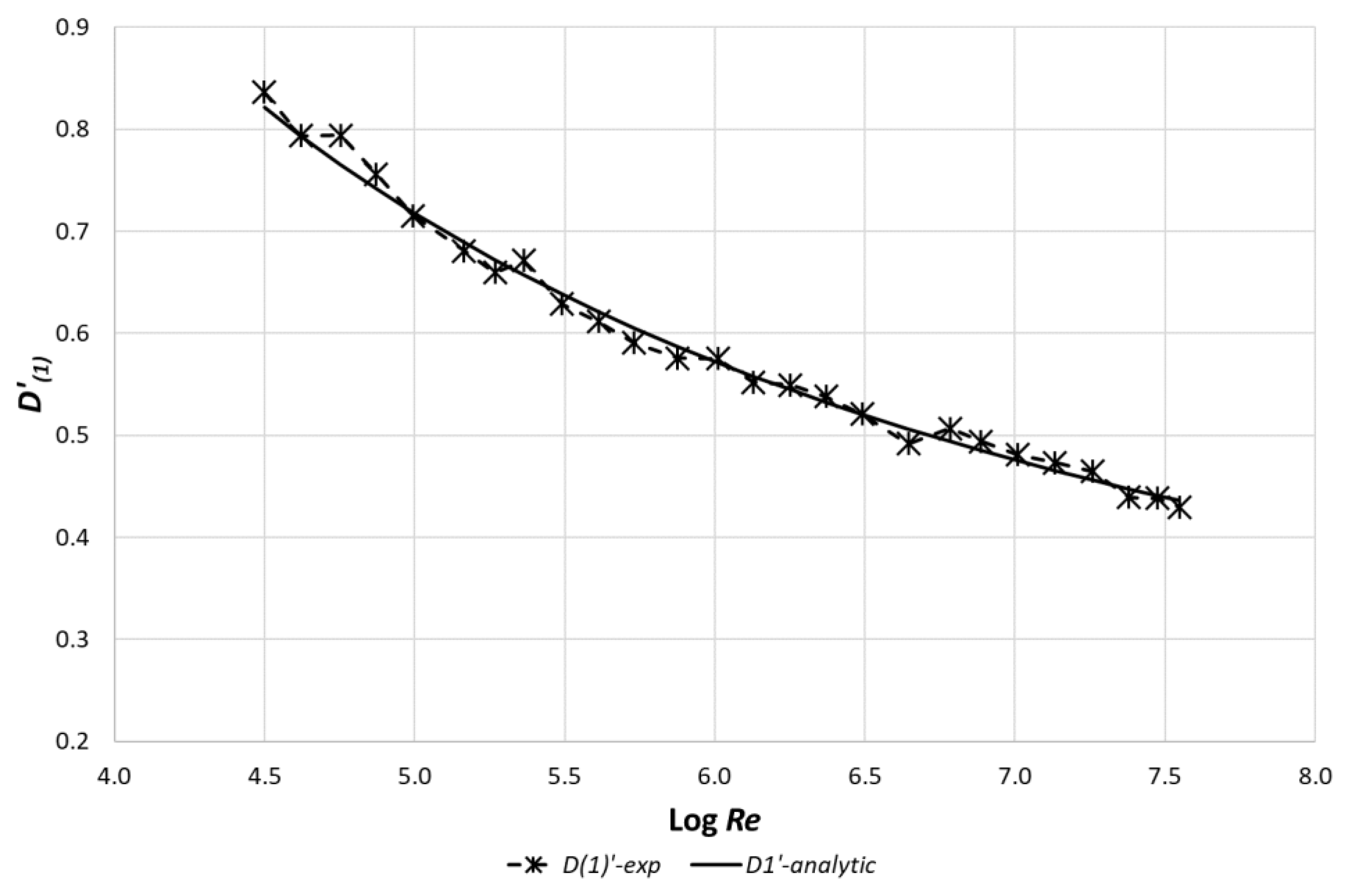
It was already mentioned, the first vorticity derivative (D(1)) depends on the average velocity and the density. When the density is constant, then the dependence on the average velocity is near to be linear. This is apparent from Figure 7. It is better to work with the normalized vorticity to express the derivative (D′(1)) as a Re function. The relationship between D(1) and D′(1) is expressed by (63). The dependence of D′(1) on the Re is in Figure 18. The dashed line with the stars represents the data obtained from the experiments. The solid line is the analytical expression of this dependence.
The analytical expression is as follows:
where A(D1) = 2.832 and B(D1) = −1.053. It seems that the analytical expression agrees rather well with the experimental data.
9. The Dependence of Exponents K and N on the Re
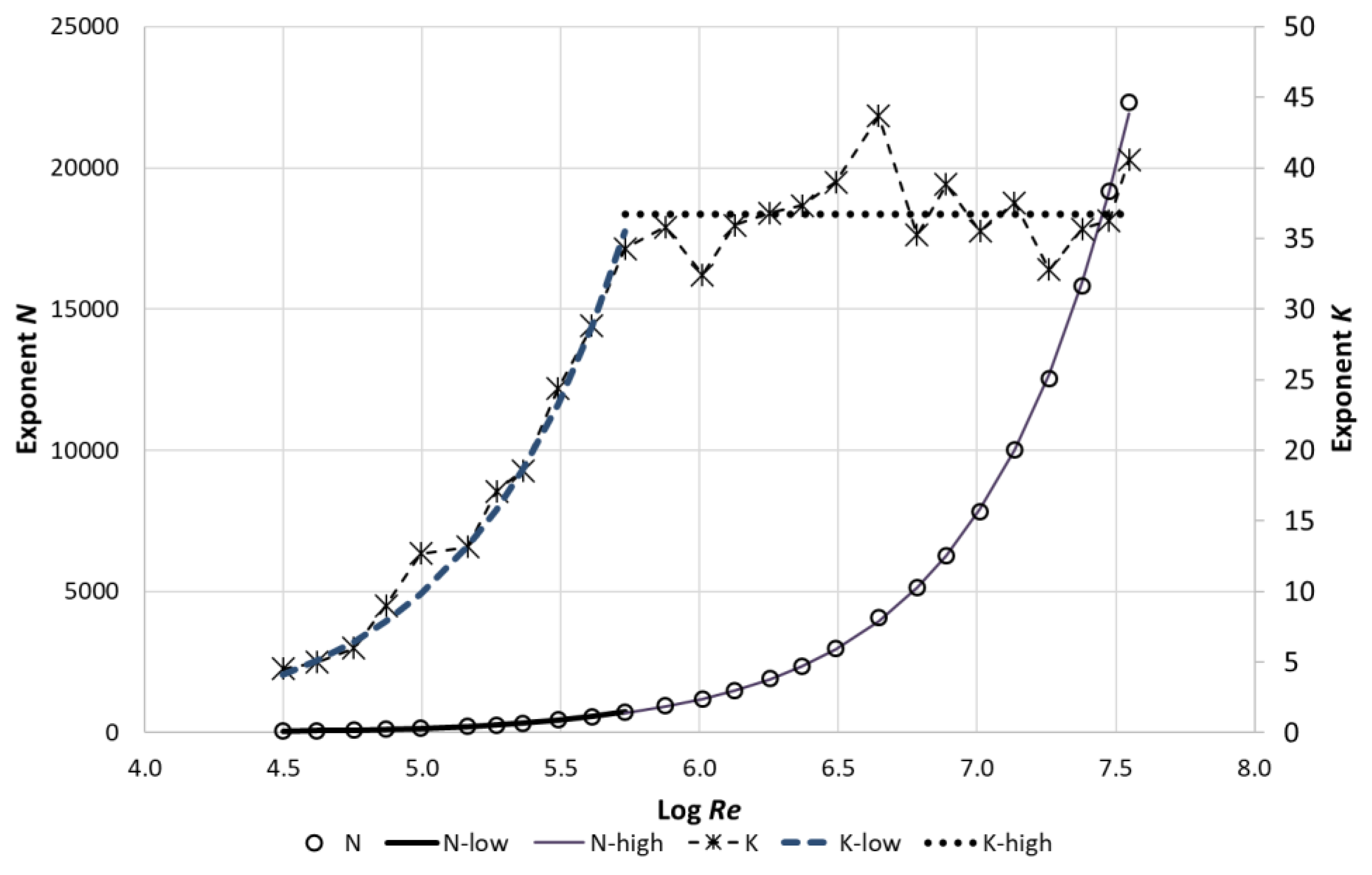
The dependences of K and N exponents on the Re are shown in Figure 19. The exponent values were originally obtained from the velocity difference minimization for the case of two variables entering into the minimization process. The values of the K exponent are drawn by stars and the values of the N exponent are drawn by empty circles in Figure 19. Analytical expressions of these dependences can be expressed for two Re intervals. First interval for Re is <31,500, 550,000> and second interval is <550,000, 35,259,000>. The expressions for K exponents follow:
where A(eK) = 0.757628 and B(eK) = 620.062.
The expressions for the exponent N are
where A(eN1) = 0.9038382, B(eN1) = 205.532, A(eN2) = 0.823883 and B(eN2) = 75.3454.
10. Mean Velocity Profile Prediction
Two methods of the mean velocity profile prediction will be demonstrated in this section. In the first way, it will be assumed that all characteristics of the mean velocity profile are known and the empirical expressions for the exponents will be applied. The solutions are shown in Figure 20 and Figure 21. The results for low Re are in Figure 20 and the results for high Re are in Figure 21.
The second way, the worst one, is that only the average velocity v(av), the pipe radius R, and viscosity are known. All other parameters are obtained with the help of empirical expressions. This solution for low and high Re is shown in Figure 22 and Figure 23. The analytical mean velocity precession is evaluated through the average absolute difference percentage s (64). The precession comparison is in Table 3.
It is apparent from Table 3 that the predicted mean velocity profiles are not bad. There is even the precession increasing for high Re in case of the second way of prediction.
11. Conclusions
The new analytical formula for the turbulent mean velocity profile in the pipe with a circular cross section is presented in this paper. This formula is derived on the basis of the induced velocity by the cylindrical vortex sheets. This paper discusses all possible boundary conditions in the paper. Two new conditions, the second velocity derivative (the first vorticity derivative) in the pipe axis and the average velocity radius, are introduced here. Values of the four free parameters in the analytical formula are derived as a function of the wall vorticity Ω(w), average velocity v(av), maximal velocity v(max), and the first vorticity derivative in the pipe axis D(1). The condition of the average velocity radius has not been used yet. The analytical expression of the mean velocity profile is defined by the Expressions (48)–(57). There are two unknown exponents K and N in the formula. The values of these exponents can be obtained by the minimization process of the velocity difference between the analytical velocity and the experimental data. The important fact is that during the minimization process the mean velocity profile characteristics are constant. The exponents K and N can be expressed as Re functions by the empirical formulas (69) and (70). If only the average velocity, pipe radius, and Re are known, then it is possible to use Expressions (36), (67), and (68) for the values of v’(max), Ω′(w), and D′(1). Two examples of mean velocity profile prediction are demonstrated at the end of the paper. It was found that the prediction precision, in comparison with experimental data PSP, is very good.
All results are based on the experimental data PSP only. It means that it is necessary to do more mean velocity profile measurements to improve the empirical expressions in this model.
It will be also desirable to apply this analytical model to the lower Re close to the transition between laminar and turbulent flow, but it is necessary to do more experiments.
The advantage of this analytical velocity profile is the easy using of this formula. There is information for all the necessary parameters determination in the paper. The next important idea is that the solution is based on the vorticity flow theory. It allows for the extension of this approach to other fluid flow problems.
12. Future Work
As mentioned before, the exponents K and N are determined through the optimization process where the absolute velocity difference is minimized. Another way comes into consideration. One of the conditions has not been used yet. It is the average velocity radius condition. This condition could be used for the exponents K and N determining. However, it will be probably necessary to find another additional condition to this one. If it works, then it will not be necessary to use the minimization process for the empirical formulas of the exponents K and N.
The idea which has been presented in this paper is also applicable for the mean velocity profiles in pipes with noncircular cross sections. There is some attempt to find an analytical mean velocity profile for the pipe with the annular cross section [10]. The formula used there is not so usable because there is used the different function for the vorticity distribution. Nevertheless, there is a lot of interesting information about acceptable conditions which can be used for the velocity profile derivation. Another attempt for the expression of the mean velocity profile in a pipe with the rectangular cross-section is in [9].
Funding
Research founded by Ministerstvo Školství, Mládeže a Tělovýchovy (CZ.02.1.01/0.0/0.0/16_026/0008392) | Vysoké Učení Technické v Brně (FSI-S-20-6235).
Institutional Review Board Statement
Not applicable.
Informed Consent Statement
Not applicable.
Data Availability Statement
The link for PSP data which were analyzed in this paper is https://www.princeton.edu/~gasdyn/#superpipe_data.
Acknowledgments
Project “Computer Simulations for Effective Low-Emission Energy Engineering” No. CZ.02.1.01/0.0/0.0/16_026/0008392 by Operational Programme Research, Development and Education, Priority axis 1: Strengthening capacity for high-quality research is gratefully acknowledged for the support of the research. Project no. FSI-S-20-6235 “The Fluid Mechanics Principle Application as a Sustainable Development Tool”.
Conflicts of Interest
The authors declare no conflict of interest.
References
- Munson, B.R.; Young, D.F.; Okiishi, T.H. Fundamentals of Fluid Mechanics, 5th ed.; John Wiley & Sons, Inc.: New York, NY, USA, 2006; ISBN 978-0-471-67582-2. [Google Scholar]
- Matas, R.; Cibera, V.; Syka, T.; Vít, T. Modelling of flow in pipes and ultrasonic flowmeter bodies. EPJ Web. Conf. 2014, 67, 6. [Google Scholar] [CrossRef] [Green Version]
- Zagarola, M.V.; Smits, A.J. Mean-flow scaling of turbulent pipe flow. J. Fluid Mech. 1998, 373, 33–79. [Google Scholar] [CrossRef]
- Cantwell, B.J. A universal velocity profile for smooth wall pipe flow. J. Fluid Mech. 2019, 878, 834–874. [Google Scholar] [CrossRef] [Green Version]
- Field, M.S.; Schiesser, W.E. Modeling solute reactivity in a phreatic solution conduit penetrating a karst aquifer. J. Contam. Hydrol. 2018, 217, 52–70. [Google Scholar] [CrossRef] [PubMed]
- Stewart, J. Calculus: Early Transcendentals, 7th ed.; Brooks/Cole Cengage Learning: Belmont, CA, USA, 2012; ISBN 978-0-538-49790-9. [Google Scholar]
- Alekseenko, S.V.; Kuibin, P.A.; Okulov, V.L. Theory of Concentrated Vortices: An Introduction; Springer: New York, NY, USA, 2007; ISBN 978-3-540-73375-1. [Google Scholar]
- Štigler, J. Contribution to investigation of turbulent mean-flow velocity profile in pipe of circular cross-section. In Proceedings of the 35th Meeting of Departments of Fluid Mechanics and Thermomechanics; AIP Publishing: Šamorín, Slovak Republic, 2016; pp. 1–13. [Google Scholar] [CrossRef] [Green Version]
- Soukup, L. Analysis of the Fluid Flow in Pipes Circular and not Circular Cross-Section with the Methods Using Distribution of the Vorticity Density. Ph.D. Thesis, Faculty of Mechanical Engineering, Energy Institute, Brno University of Technology, Brno, Czech Republic, December 2016. [Google Scholar]
- Bartková, T. Fluid Flow in Narrow gap Between two Cylinders Induced by Pressure Gradient. Master’s Thesis, Faculty of Mechanical Engineering, Energy institute, Brno University of Technology, Brno, Czech Republic, July 2020. [Google Scholar]
Figure 1.
A vortex filament and an infinitesimal velocity induced by a vortex filament element.

Figure 2.
Velocity induced by an infinite cylindrical vortex sheet.

Figure 3.
Interaction of two concentric circular vortex sheets.

Figure 4.
A vorticity distribution over the pipe cross-section.

Figure 5.
Pressure and friction forces in the pipe.

Figure 6.
Normalized mean velocity profile acquired by experiment (PSP) and the corresponding normalized vorticity distribution over cross-section for Re = 230,460. (a) Normalized mean velocity profile; (b) Normalized vorticity distribution.
Figure 6.
Normalized mean velocity profile acquired by experiment (PSP) and the corresponding normalized vorticity distribution over cross-section for Re = 230,460. (a) Normalized mean velocity profile; (b) Normalized vorticity distribution.

Figure 7.
The dependence of the first vorticity derivative in the axis on the average velocity for different densities.
Figure 7.
The dependence of the first vorticity derivative in the axis on the average velocity for different densities.

Figure 8.
The dependence of the normalized maximal velocity on the Re.

Figure 9.
All mean velocity profiles measured by Zagarola [3] on PSP. There are 26 profiles for the Reynold’s number range <31,577, 35,259,000>.
Figure 9.
All mean velocity profiles measured by Zagarola [3] on PSP. There are 26 profiles for the Reynold’s number range <31,577, 35,259,000>.

Figure 10.
The average velocity radius for all 26 velocity profiles measured by Zagarola [3] on PSP.
Figure 10.
The average velocity radius for all 26 velocity profiles measured by Zagarola [3] on PSP.

Figure 11.
The analytical formula comparison with the experimental data (PSP) for Re = 31,577, using K and N as the variables. Dashed line with circles represents the experimental data, the solid line is the analytical profile. (a) Normalized mean velocity profile, (b) Normalized vorticity distribution.

Figure 12.
The analytical formula comparison with the experimental data (PSP) for Re = 13,598,000, using K and N as the variables. Dashed line with circles represents the experimental data, the solid line is the analytical profile. (a) Normalized mean velocity profile, (b) Normalized vorticity distribution.

Figure 13.
The analytical formula comparison with the experimental data (PSP) for Re = 31,577, using variables Ω(w), D(1), K, and N. Dashed line with circles represents the experimental data, the solid line is the analytical profile. (a) Normalized mean velocity profile, (b) Normalized vorticity distribution.

Figure 14.
The analytical formula comparison with the experimental data (PSP) for Re = 13,598,000, using variables Ω(w), D(1), K, and N. Dashed line with circles represents the experimental data, the solid line is the analytical profile. (a) Normalized mean velocity profile, (b) Normalized vorticity distribution.

Figure 15.
The velocity profiles in the coordinates u+, y+. (a) The case of two variables N and K in the optimization process. (b) The case of four variables Ω(w), D(1), N, and K in the optimization process.
Figure 15.
The velocity profiles in the coordinates u+, y+. (a) The case of two variables N and K in the optimization process. (b) The case of four variables Ω(w), D(1), N, and K in the optimization process.

Figure 16.
The comparison of the normalized wall vorticity obtained by four variables optimization with experimental data.
Figure 16.
The comparison of the normalized wall vorticity obtained by four variables optimization with experimental data.

Figure 17.
The comparison of the analytical expressions for Ω′(w) with the experimental data.

Figure 18.
The comparison of the analytical expressions for D′(1) with the experimental data.

Figure 19.
The dependence of K and N exponents on the Re.

Figure 20.
The experimental data (PSP) for Re = 31,577 comparison with predicted mean velocity profile. The empirical formulas for exponents K and N are used only. Dashed line with circles represents the experimental data, the solid line is the analytical profile. (a) Normalized mean velocity profile, (b) Normalized vorticity distribution.

Figure 21.
The experimental data (PSP) for Re = 13,598,000 comparison with predicted mean velocity profile. The empirical formulas for exponents K and N are used only. Dashed line with circles represents the experimental data, the solid line is the analytical profile. (a) Normalized mean velocity profile, (b) Normalized vorticity distribution analytical.

Figure 22.
The experimental data (PSP) for Re = 31,577 comparison with predicted mean velocity profile. The average velocity and Re are known in this case. All other parameters are evaluated from the empirical expressions. Dashed line with circles represents the experimental data, the solid line is the analytical profile. (a) Normalized mean velocity profile, (b) Normalized vorticity distribution.

Figure 23.
The experimental data (PSP) for Re = 13,598,000 comparison with predicted mean velocity profile. The average velocity and Re are known in this case. All other parameters are evaluated from the empirical expressions. Dashed line with circles represents the experimental data, the solid line is the analytical profile. (a) Normalized mean velocity profile, (b) Normalized vorticity distribution.


Table 1.
Parameters of the analytical velocity profile. Exponents K and N are obtained from comparison with the experimental data.
Table 1.
Parameters of the analytical velocity profile. Exponents K and N are obtained from comparison with the experimental data.
| p.n. | Re [1] | v(av) [m.s−1] | v(max) [m.s−1] | Ω(w) [s−1] | D(1) [m−1.s−1] | N [-] | K [-] | Ω′(w) [1] | D‘(1) [1] | v‘(max) [1] |
|---|---|---|---|---|---|---|---|---|---|---|
| 01 | 31,577 | 3.876 | 4.821 | 2748 | 775 | 55.3 | 4.5 | 45.9 | 0.8363 | 1.2439 |
| 02 | 41,727 | 5.132 | 6.351 | 4523 | 974 | 71.5 | 5.0 | 57.0 | 0.7939 | 1.2374 |
| 03 | 56,677 | 6.845 | 8.410 | 7639 | 1299 | 95.7 | 6.0 | 72.2 | 0.7941 | 1.2287 |
| 04 | 74,293 | 8.952 | 10.926 | 12,288 | 1618 | 120.9 | 9.0 | 88.8 | 0.7562 | 1.2204 |
| 05 | 98,811 | 11.896 | 14.404 | 20,447 | 2032 | 159.9 | 12.7 | 111.3 | 0.7151 | 1.2118 |
| 06 | 145,790 | 17.532 | 21.011 | 41,029 | 2853 | 223.5 | 13.1 | 151.4 | 0.6808 | 1.1984 |
| 07 | 185,430 | 22.623 | 26.976 | 64,189 | 3567 | 280.5 | 17.1 | 183.5 | 0.6596 | 1.1924 |
| 08 | 230,460 | 9.751 | 11.58 | 32,974 | 1565 | 340.1 | 18.6 | 218.7 | 0.6715 | 1.1875 |
| 09 | 309,500 | 13.110 | 15.489 | 56,885 | 1971 | 449.8 | 24.4 | 280.7 | 0.6289 | 1.1815 |
| 10 | 409,290 | 17.357 | 20.405 | 94,436 | 2537 | 575.6 | 28.8 | 351.9 | 0.6116 | 1.1756 |
| 11 | 539,090 | 22.840 | 26.768 | 156,752 | 3225 | 737.3 | 34.3 | 443.9 | 0.5908 | 1.1720 |
| 12 | 751820 | 6.271 | 7.327 | 56,744 | 863 | 955.1 | 35.8 | 585.2 | 0.5757 | 1.1683 |
| 13 | 1,023,800 | 8.440 | 9.820 | 98,752 | 1161 | 1208.0 | 32.4 | 756.9 | 0.5754 | 1.1636 |
| 14 | 1,340,400 | 11.071 | 12.851 | 162,559 | 1461 | 1504.3 | 35.9 | 949.7 | 0.5519 | 1.1608 |
| 15 | 1,787,500 | 14.769 | 17.110 | 276,184 | 1940 | 1915.6 | 36.8 | 1209.5 | 0.5495 | 1.1585 |
| 16 | 2,345,000 | 19.478 | 22.493 | 456,420 | 2506 | 2354.0 | 37.3 | 1515.6 | 0.5382 | 1.1548 |
| 17 | 3,098,100 | 13.268 | 15.280 | 395,546 | 1652 | 2974.4 | 39.0 | 1928.2 | 0.5208 | 1.1516 |
| 18 | 4,420,300 | 5.081 | 5.830 | 205,830 | 597 | 4064.6 | 43.7 | 2620.3 | 0.4920 | 1.1474 |
| 19 | 6,072,700 | 6.928 | 7.931 | 368,398 | 839 | 5126.3 | 35.2 | 3439.3 | 0.5068 | 1.1447 |
| 20 | 7,714,700 | 6.580 | 7.523 | 427,544 | 777 | 6262.6 | 38.8 | 4202.4 | 0.4941 | 1.1432 |
| 21 | 10,249,000 | 8.703 | 9.917 | 719,643 | 1001 | 7815.3 | 35.5 | 5348.3 | 0.4810 | 1.1395 |
| 22 | 13,598,000 | 11.504 | 13.083 | 1,220,866 | 1302 | 10,002.3 | 37.5 | 6864.2 | 0.4733 | 1.1373 |
| 23 | 18,196,000 | 15.345 | 17.358 | 2,093,107 | 1705 | 12,541.5 | 32.8 | 8822.6 | 0.4647 | 1.1312 |
| 24 | 23,977,000 | 20.149 | 22.758 | 3,499,514 | 2115 | 15,818.9 | 35.7 | 11,233.7 | 0.4391 | 1.1295 |
| 25 | 29,927,000 | 25.043 | 28.265 | 5,295,477 | 2623 | 19,157.9 | 36.3 | 13,676.9 | 0.4382 | 1.1287 |
| 26 | 35,259,000 | 29.306 | 33.087 | 7,180,224 | 3010 | 22,306.5 | 40.6 | 15,847.2 | 0.4297 | 1.1290 |
Table 2.
Parameters of the analytical velocity profile. Quantities Ω(w), D(1), N, and K are obtained from comparison with the experimental data.
Table 2.
Parameters of the analytical velocity profile. Quantities Ω(w), D(1), N, and K are obtained from comparison with the experimental data.
| p.n. | Re [1] | v(av) [m.s−1] | v(max) [m.s−1] | Ω(w) [s−1] | D(1) [m−1.s−1] | N [-] | K [-] | Ω′(w) [1] | D′(1) [1] | v′(max) [1] |
|---|---|---|---|---|---|---|---|---|---|---|
| 01 | 31,577 | 3.876 | 4.821 | 3606 | 1156 | 82.2 | 4.0 | 60.2 | 1.2475 | 1.2439 |
| 02 | 41,727 | 5.132 | 6.351 | 6183 | 1420 | 109.9 | 5.1 | 77.9 | 1.1579 | 1.2374 |
| 03 | 56,677 | 6.845 | 8.410 | 10,480 | 1560 | 146.8 | 10.0 | 99.0 | 0.9532 | 1.2287 |
| 04 | 74,293 | 8.953 | 10.926 | 16,677 | 1881 | 180.1 | 11.0 | 120.5 | 0.8789 | 1.2204 |
| 05 | 98,811 | 11.886 | 14.404 | 27,207 | 1969 | 229.3 | 19.7 | 148.1 | 0.6929 | 1.2118 |
| 06 | 145,790 | 17.532 | 21.011 | 52,502 | 2654 | 307.2 | 22.7 | 193.7 | 0.6332 | 1.1984 |
| 07 | 185,430 | 22.623 | 26.976 | 73,314 | 3313 | 329.6 | 22.2 | 209.6 | 0.6126 | 1.1924 |
| 08 | 230,460 | 9.752 | 11.580 | 36,037 | 1353 | 382.3 | 26.2 | 239.0 | 0.5805 | 1.1875 |
| 09 | 309,500 | 13.110 | 15.489 | 51,500 | 1825 | 400.6 | 25.2 | 254.1 | 0.5824 | 1.1815 |
| 10 | 409,290 | 17.357 | 20.405 | 68,893 | 2310 | 401.3 | 27.1 | 256.7 | 0.5567 | 1.1756 |
| 11 | 539,090 | 22.840 | 26.768 | 94,562 | 3076 | 422.1 | 30.3 | 267.8 | 0.5634 | 1.1720 |
| 12 | 751,820 | 6.271 | 7.327 | 39,572 | 815 | 660.0 | 37.2 | 408.1 | 0.5440 | 1.1683 |
| 13 | 1,023,800 | 8.439 | 9.820 | 80,881 | 1133 | 994.2 | 34.9 | 619.9 | 0.5615 | 1.1636 |
| 14 | 1,340,400 | 11.071 | 12.851 | 135,828 | 1456 | 1254.0 | 35.8 | 793.5 | 0.5502 | 1.1608 |
| 15 | 1,787,500 | 14.769 | 17.110 | 226,335 | 1952 | 1563.6 | 35.8 | 991.2 | 0.5528 | 1.1585 |
| 16 | 2,345,000 | 19.478 | 22.493 | 374,371 | 2527 | 1926.3 | 36.7 | 1,243.2 | 0.5427 | 1.1548 |
| 17 | 3,098,100 | 13.268 | 15.280 | 353,477 | 1658 | 2652.4 | 38.6 | 1,723.2 | 0.5227 | 1.1516 |
| 18 | 4,420,300 | 5.081 | 5.830 | 181,425 | 617 | 3554.7 | 40.9 | 2,309.6 | 0.5084 | 1.1474 |
| 19 | 6,072,700 | 6.928 | 7.931 | 318,384 | 835 | 4427.3 | 35.3 | 2,972.4 | 0.5044 | 1.1447 |
| 20 | 7,714,700 | 6.580 | 7.523 | 375,852 | 781 | 5501.9 | 38.5 | 3,694.3 | 0.4963 | 1.1432 |
| 21 | 10,249,000 | 8.703 | 9.917 | 597,357 | 1010 | 6495.2 | 35.6 | 4,439.5 | 0.4853 | 1.1395 |
| 22 | 13,598,000 | 11.504 | 13.083 | 1,104,237 | 1332 | 8983.2 | 34.6 | 6,208.5 | 0.4844 | 1.1373 |
| 23 | 18,196,000 | 15.345 | 17.358 | 1,812,336 | 1669 | 10,839.6 | 32.7 | 7,639.1 | 0.4550 | 1.1312 |
| 24 | 23,977,000 | 20.149 | 22.758 | 2,476,268 | 2041 | 11,258.8 | 40.3 | 7,949.0 | 0.4238 | 1.1295 |
| 25 | 29,927,000 | 25.043 | 28.265 | 4,757,948 | 2661 | 17,202.4 | 35.5 | 12,288.6 | 0.4446 | 1.1287 |
| 26 | 35,259,000 | 29.306 | 33.087 | 6,549,529 | 3293 | 20,042.4 | 31.9 | 14,455.2 | 0.4701 | 1.1290 |
Table 3.
The mean velocity profile precession comparison for different ways of prediction. The comparison is done through the value δ.
Table 3.
The mean velocity profile precession comparison for different ways of prediction. The comparison is done through the value δ.
| Analytical Velocity Profile | δ [% of v(av)] | |
|---|---|---|
| Re = 31,577 | Re = 13,598,000 | |
| Minimization variables K, and N | 2.183 | 0.364 |
| Minimization variables Ω(w), D(1), K, and N | 0.494 | 0.362 |
| The first prediction way | 2.210 | 0.377 |
| The second prediction way | 2.783 | 0.339 |
Publisher’s Note: MDPI stays neutral with regard to jurisdictional claims in published maps and institutional affiliations. |
© 2021 by the author. Licensee MDPI, Basel, Switzerland. This article is an open access article distributed under the terms and conditions of the Creative Commons Attribution (CC BY) license (https://creativecommons.org/licenses/by/4.0/).
Share and Cite
MDPI and ACS Style
Štigler, J. Analytical Formula for the Mean Velocity Profile in a Pipe Derived on the Basis of a Spatial Polynomial Vorticity Distribution. Water 2021, 13, 1372. https://doi.org/10.3390/w13101372
AMA Style
Štigler J. Analytical Formula for the Mean Velocity Profile in a Pipe Derived on the Basis of a Spatial Polynomial Vorticity Distribution. Water. 2021; 13(10):1372. https://doi.org/10.3390/w13101372
Chicago/Turabian StyleŠtigler, Jaroslav. 2021. "Analytical Formula for the Mean Velocity Profile in a Pipe Derived on the Basis of a Spatial Polynomial Vorticity Distribution" Water 13, no. 10: 1372. https://doi.org/10.3390/w13101372
Note that from the first issue of 2016, this journal uses article numbers instead of page numbers. See further details here.