Study on the Exploitation Scheme of Groundwater under Well-Canal Conjunctive Irrigation in Seasonally Freezing-Thawing Agricultural Areas

Abstract

The suitable groundwater exploitation scheme in freezing-thawing agricultural areas under the well-canal conjunctive irrigation conditions is confronted with two major challenges, which are computationally expensive local grid refinements along wells, and the model suitability problem in the freezing-thawing period. In this study, an empirical method for groundwater level prediction in the freezing-thawing period was developed and integrated with the local grid refinement groundwater model MODFLOW-LGR for the groundwater process prediction. The model was then applied to estimate the suitable groundwater exploitation scheme, including the size of well-irrigated area and the irrigation area of single well. The results showed that suitable size of well-irrigated area should be smaller than 15 × 10⁶ m², and the recommended irrigation area of single well as 15 × 10⁴ m² to 19 × 10⁴ m². The recommended layout parameters of groundwater exploitation were further used to plan the well-canal conjunctive irrigation scheme in Yongji irrigation district located in northern China. This study provides an important pilot example of the conjunctive use of groundwater and surface water in arid irrigation areas with a seasonal freezing-thawing period.

1. Introduction

In the past several decades, there has been a growing threat to the sustainability of water resources, especially in arid and semi-arid regions, because of over-urbanization, increasing irrigation demands, and climate change impacts [1,2]. One important aspect of water resources sustainability is the efficient utilization of agricultural water since it consumes the largest portion of freshwater resource around the world [3,4]. Well-canal conjunctive irrigation system is one of the most promising schemes, as it can alleviate the shortage and uncertain supplies of surface water resources in arid and semi-arid agricultural areas [5]. Besides, many agricultural areas in arid and semi-arid regions tend to have small groundwater table depth due to the crude surface water irrigation practices, which result in significant phreatic evaporation and secondary soil salinization [6]. The exploitation of groundwater resources can decrease the ineffective phreatic evaporation, which increases water-use efficiency [7,8,9,10,11,12] and prevents the deterioration of soil salinization [13,14]. The well-canal conjunctive systems have been used in many agricultural areas [15,16,17]. However, the system might have adverse effects such as groundwater depression cone and soil desertification if over-exploitation happens [18,19]. Therefore, the suitable groundwater exploitation scheme is the core question for the well-canal conjunctive irrigation system in the regional-scale agricultural areas.

Hetao Irrigation District is a typical arid agricultural area, which is located in the Inner Mongolia Autonomous Region, China, and the average annual evaporation from 20 cm pan (2329 mm) is almost 14 times greater than the average annual precipitation (169 mm). As a result, the area heavily relies on water diversion (with an average of 844 million m³/y) from the Yellow River for irrigation. Since the diversion allocation from the Yellow River will be reduced for the irrigation district and the groundwater resources are barely being exploited, well-canal conjunctive irrigation has been considered as the major scheme for sustainable agriculture development in the Hetao Irrigation District [20,21], and its implementation is already on the agenda. Therefore, a thorough study for the suitable groundwater exploitation scheme under well-canal conjunctive irrigation in Hetao Irrigation District is essential.

Many studies have been conducted to study the effectiveness and efficiency of well-canal conjunctive irrigation schemes and the groundwater and salinity dynamics under different conjunctive scenarios [22,23,24,25,26]. Various optimization methods have been developed to determine the optimal well layout parameters, including well numbers, locations and pumping rates [27,28,29,30,31,32]. The numerical models, such as MODFLOW and other simulation models (e.g., Penn State Integrated Hydrologic Model (PIHM) and FEFLOW), do well in simulating groundwater drawdowns and changes of groundwater recharge under groundwater pumping conditions on a regional scale, and are perfectly suitable for the well-canal conjunctive irrigation problem [33,34,35,36,37,38]. However, current studies mainly focus on groundwater decline under regional average conditions [39,40,41,42,43], which fails to accurately represent the more pronounced local groundwater level decline adjacent to wells. The simulation of the groundwater local cone of depression around wells requires very fine local grids to improve simulation accuracy and assess the risk of decreased groundwater level. Three major methods of local grid refinement are developed for finite difference models, which are the gradational mesh refinement (GMR), telescopic mesh refinement (TMR) and local grid refinement (LGR). The GMR is criticized for its numerical instabilities due to the large aspect ratio of cells [44]. TMR is a one-way coupling method, and requires modelers developing methods to assess and redress consistency of results along boundary interfaces, which could result in undetected errors [45]. Comparing with GMR and TMR, LGR is more rigorous, because it uses a two-way iterative coupling method to link parent and child grids [46]. Therefore, the LGR method is more suitable to refine the finite difference grids around pumping wells for a more accurate prediction when considering the groundwater exploitation of the well-irrigated area.

Another concern is the freezing and thawing processes in Hetao Irrigation District. There is a five-months freezing-thawing period from December to April of the next year in this area [47]. In the freezing period, the soil water gradually freezes downward from the surface, causing the groundwater discharges to the vadose zone driven by the negative pore-water pressure and groundwater level decreases, while in the thawing period, the frozen soil begins to melt, causing the soil water to recharge aquifer and the groundwater level to increase. The processes of moisture migration, freezing processes, and heat transfer are highly correlated during the freezing-thawing period, which can directly affect numerous hydrogeological processes, including thermal regimes, groundwater flow patterns, and groundwater recharges [48,49]. The present physically based regional-scale groundwater models (e.g., MODFLOW and PIHM) cannot consider the influence of freezing and thawing processes, and thus cannot predict inter-annual groundwater in seasonally freezing-thawing agricultural areas. In addition, models developed to simulate water flow and heat transport for systems undergoing freezing-thawing mainly focus on a saturated porous medium, such as SUTRA, SMOKER, and MELT [50,51,52,53]. These models assume that the porous medium is fully saturated with water while ignoring the phase change of water between saturated and unsaturated zones, which render these models not suitable for modeling phreatic water table in the seasonally freezing-thawing areas. Furthermore, there is also a freezing and thawing module developed and coupled with HYDRUS-1D [54] and applied for simulation in freezing-thawing areas [55]. However, this module focuses on the local soil water movement and fails for regional-scale groundwater simulations. Thus, an empirical method for inter-annual regional groundwater modeling in seasonally freezing-thawing areas was developed in this study to alleviate the complicated physically based processes.

In this study for groundwater exploitation, layout parameters of single wells and well-irrigated area under well-canal conjunctive irrigation in the seasonally freezing-thawing agricultural area were investigated. The denser grid adjacent to the pumping well was used for the accuracy groundwater table depth prediction with the help of MODFLOW-LGR. An empirical method was developed by establishing the relationship between groundwater recharge/discharge with temperature to describe the freezing-thawing process of the groundwater system during freezing-thawing periods. Moreover, after the calibration and validation of the numerical tools, the layout parameters of groundwater exploitation, including the size of a single well-irrigated area and the controlling irrigation area of a single well were investigated, which were further used for planning the reasonable well-canal irrigation scheme in Hetao Irrigation District.

2. Materials and Methods

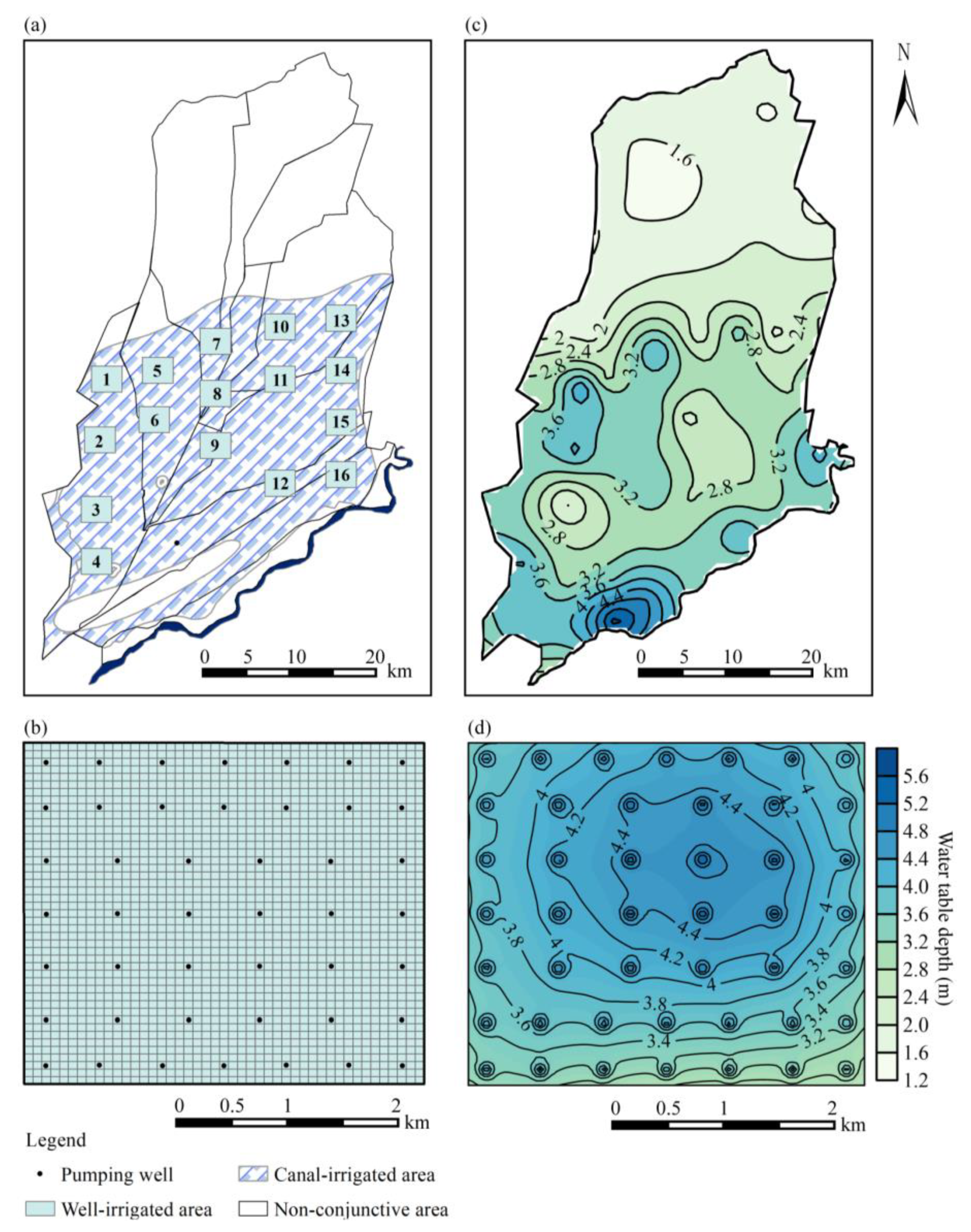
In this section, the overview of the study area was firstly presented, then the multiscale numerical model for seasonally freezing-thawing agricultural areas was introduced. The validity of the empirical method for calculating groundwater recharge/discharge during the freezing-thawing period was illustrated, and the data preparation for the study area was presented.

2.1. Study Area

The Hetao Irrigation District is the largest agricultural area in the arid region of China, and there are five sub-irrigation districts, which, from west to east, are Ulanbuh, Jiefangzha, Yongji, Yichang and Urad. Yongji sub-irrigation district is located in the middle of the Hetao Irrigation District (40°12′~41°20′ N, 106°10′~109°30′ E) as shown in Figure 1a, and the whole domain size is 1.887 × 10³ km² and is 75 km long from north to south and 44 km wide from east to west. The annual average precipitation is 137 mm while the annual average evaporation measured with the 20 cm evaporation pan is 2281 mm. The main crops in this area are wheat, corn and sunflower, which are irrigated mainly by the water diversion from the Yellow River. The aquifer can be divided into two layers. An upper, less permeable layer consists of mixed sand and clay and thickness varies between 6 and 8 m, and a lower, more permeable sandy layer has an average thickness of 121 m. There are 12 main canals and the volume of monthly diversion water of each canal were measured from 2006 to 2017 by Irrigation Bureau of Hetao Irrigation District. The daily precipitation, evaporation and temperature during 2006 to 2017 were obtained from the Linhe Weather Station, and the monthly values are shown in Figure 2. There are 45 groundwater monitoring wells used to measure the water table depth every 5 days from 2006 to 2017 in Yongji sub-irrigation district. Currently, there is a well-irrigated area in the middle of Yongji sub-irrigation district called Longsheng, where groundwater has been used for irrigation since 1999. The Longsheng well-irrigated area is about 18.1 km² with 72 pumping wells for irrigation, and the locations of these wells are presented in Figure 1c. The fraction of irrigated farmlands in this well-irrigated area is 0.58, and the actual area of irrigated farmlands is 10.5 km². The main crops are wheat, corn and sunflower, with the average irrigation quota of 681.10 mm, 579.50 mm and 336.45 mm, respectively. Eight groundwater observation wells were set up in the Longsheng well-irrigated area to observe the water table depth every 10 days from May 2017.

There is a plan to use groundwater for irrigation in Yongji sub-irrigation district for reducing surface water diversion from the Yellow River. The area with groundwater salinity less than 2.5 g/L is considered as the exploitable area of groundwater as shown in Figure 1b considering the requirement of irrigation water quality [56]. The groundwater in the well-irrigated area has a lower groundwater level caused by the well pumping, and will be recharged laterally by the groundwater in the canal-irrigated area driven by the groundwater gradient. The reasonable area ratio of canal-irrigated area over well-irrigated area to maintain the balance of groundwater exploitation and recharge in well-irrigated area is 3:1 according to the groundwater mass balance method [57]. In this study, the specific groundwater exploitation scheme, including the suitable size of one single well and well-irrigated area, and the groundwater dynamics after well-canal conjunctive irrigation will be investigated.

2.2. Multiscale Numerical Model for Seasonally Freezing-Thawing Agricultural Areas

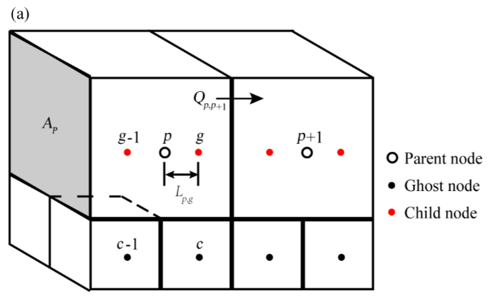
2.2.1. Multiscale Model MODFLOW-LGR

MODFLOW-LGR is designed to allow users to create MODFLOW simulations using one or more refined grids that are embedded within a coarser grid to achieve more accurate results in areas of interest [58]. The three-dimensional water flow equation is as follows,

$$\{\begin{array}{ll}\frac{\partial }{\partial x}\left(K_{xx}\frac{\partial h}{\partial x}\right)+\frac{\partial }{\partial y}\left(K_{yy}\frac{\partial h}{\partial y}\right)+\frac{\partial }{\partial z}\left(K_{zz}\frac{\partial h}{\partial z}\right)+W=S_s\frac{\partial h}{\partial t}& x,y,z\in \mathsf{\Omega }\\ {h\left(x,y,z,t\right)|}_{t=0}=h_0\left(x,y,z\right)& x,y,z\in \mathsf{\Omega }\\ {h\left(x,y,z,t\right)|}_{s_1}=\phi \left(x,y,z,t\right)& x,y,z\in s_1\\ {K\frac{\partial h}{\partial n}|}_{s_2}=\psi \left(x,y,z,t\right)& x,y,z\in s_2\end{array}$$

(1)

where K_xx, K_yy, K_zz are values of hydraulic conductivity along the x, y and z coordinate axes (L T⁻¹); h is the hydraulic head (L); W is the volumetric flux per unit volume representing source and/or sink of water (T⁻¹); S_s is the specific storage of the porous material (L⁻¹); Ω is the domain of calculated scope; h₀ is the initial hydraulic head (L); s₁ and s₂ are the boundaries of the first and second types; φ is the first type boundary condition (L); ψ is the second type boundary condition (L² T⁻¹).

There are three kinds of nodes used by MODFLOW-LGR as shown in Figure 3a, e.g., the parent node used by the parent model, the child node used by the child LGR model and the ghost node used to couple the parent and child models. The numbers of the three kinds of nodes are marked as a, b, c. Figure 3a shows the coupling procedures of MODFLOW-LGR and the iterative coupling scheme at time t. The model begins by simulating a parent model that encompasses the entire domain while ignoring the child model domain to obtain the hydraulic head of the parent nodes at time t and at the j-th LGR iteration, marked as ${(h_p)}_t^j$ (a dimension). The ghost nodes are set at the cells of the parent model which are adjacent to the child model domain. The hydraulic heads of the ghost nodes are calculated by the interpolation of the parent nodes, marked as ${(h_g)}_t^j$ (c dimension). The ${(h_g)}_t^j$ term is calculated as follows,

$$h_g=h_p-\frac{Q_{p,p+1}{L}_{p,g}}{K_p{A}_p}$$

(2)

where h_g and h_p are the hydraulic head of the ghost node and the parent node (L); Q_p,p+1 is the flow between two adjacent parent cells (L³ T⁻¹); K_p is the hydraulic conductivity of the parent cell (L T⁻¹); A_p is the cross-sectional area of the parent cell perpendicular to flow (L²); L_p,g is the distance between the parent node and the ghost node (L).

The hydraulic heads of the ghost nodes are considered as the specified boundary condition for the child model. The child model is then run to obtain the hydraulic head of the child nodes, marked as ${(h_c)}_t^j$ (b dimension). Then the flux through the interface of the parent and child model domain can be calculated by the head difference between the ghost node and the adjacent child node. The flux is marked as ${(Q_E)}_t^j$ (c dimension). The item of ${(Q_E)}_t^j$ is calculated as follows,

$$Q_E=C_{g-1}\left(h_{g-1}-h_{c-1}\right)+C_g\left(h_g-h_c\right)$$

(3)

where Q_E is the specified flux for the parent node (L³ T⁻¹); C_g is the hydraulic conductance of the ghost node (L² T⁻¹); h_c is the hydraulic head of the child node (L).

The parent model is re-run under this updated flux boundary conditions and produces updated hydraulic heads of parent nodes, marked as ${(h_p)}_t^{j+1}$. Subsequently, the updated hydraulic head of the ghost nodes ${(h_g)}_t^{j+1}$, the updated hydraulic head of the child nodes ${(h_c)}_t^{j+1}$, and the interface flux ${(Q_E)}_t^{j+1}$ can be obtained. This process is repeated until the maximum change of the hydraulic head of the ghost nodes and the flux at the interface are smaller than user-defined criteria. The convergence criteria are

$$\max \left(\left|{(h_g)}_t^{j+1}-{(h_g)}_t^j\right|\right)<{\epsilon }_h$$

(4)

$$\max \left(\left|{(Q_E)}_t^{j+1}-{(Q_E)}_t^j\right|\right)<{\epsilon }_Q$$

(5)

where ε_h and ε_Q are the user-defined criteria, which were set as 0.005 m and 0.05 m³/d in this study.

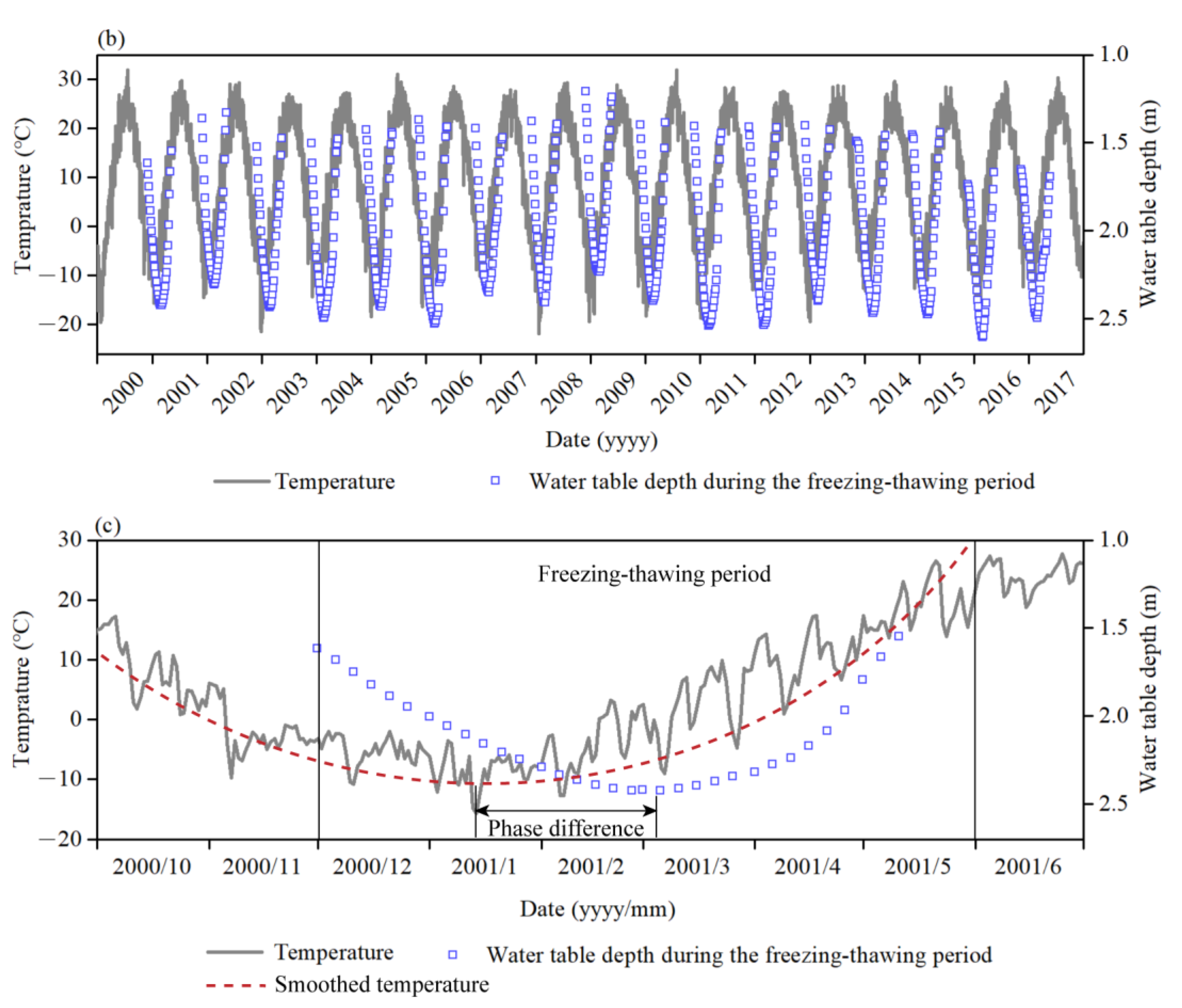
2.2.2. The Empirical Method of Calculating Groundwater Recharge/Discharge during the Freezing-Thawing Period

Groundwater hydrological processes are mainly influenced by air temperatures during the freezing-thawing period in agricultural areas with water table depth shallower than 1.8 m [59]. As the temperature decreases in the freezing period, the soil water gradually freezes downward from the surface, causing the liquid phase water to reduce and the negative pore-water pressure to increase. As a result, groundwater flows upwards to the freezing soil and the water table depth continues to decrease. In the thawing period, the frozen soil begins to melt from the surface as temperature rises to resupply groundwater, and the water table depth decreases. The measured daily temperature and spatially averaging groundwater table depth in the freezing-thawing period of Hetao Irrigation District are shown in Figure 3b.

Based on the synchronized variation of air temperature and water table depth shown in Figure 3b, an empirical method was developed to correlate the groundwater recharge/discharge flux with the air temperature. The temperature-time curve and water table depth-time curve are both fitted by the trigonometric function as follows,

$$T={\alpha }_T\cos \left(\frac{2\pi t}{T_0}+{\beta }_T\right)+{\gamma }_T$$

(6)

$$H=H_0+{\alpha }_H\cos \left(\frac{2\pi t}{T_0}+{\beta }_H\right)+{\gamma }_H$$

(7)

where T is the temperature (K); t is the time (T); H is the water table depth (L); H₀ is the initial water table depth of the freezing-thawing period (L); T₀ is the period, 365 d; [α_T, β_T, γ_T] are the parameters to fit the temperature-time curve (K, –, K); [α_H, β_H, γ_H] are the parameters to fit the water table depth-time curve (L, –, L).

The water table depth and temperature have the same changing cycle in the freezing-thawing period with a phase difference as Figure 3c shows, which is the lag day of the influence of air temperature on the water table depth. It can be calculated by Equation (8) using the fitted parameters β_T and β_H, which means that the water table depth is related to the temperature n days ago.

$$n=\left({\beta }_T-{\beta }_H\right)T_0/2\pi$$

(8)

where n is the lagging day of the influence of temperature on water table depth.

The temperature-time curve with a backward translation of n days can be written as follows,

$$T^{\prime }={\alpha }_T\cos \left(\frac{2\pi \left(t-n\right)}{T_0}+{\beta }_T\right)+{\gamma }_T={\alpha }_T\cos \left(\frac{2\pi t}{T_0}+{\beta }_H\right)+{\gamma }_T$$

(9)

where T’ is the temperature n days ago (K). Thus, Equation (7) and (9) has the same changing cycle and phase.

Therefore, the one-to-one functional relationship between H and T’ can be written as follows,

$$H=H_0+\frac{{\alpha }_H}{{\alpha }_T}\left(T^{\prime }-{\gamma }_T\right)+{\gamma }_H$$

(10)

It should be noted that the temperature used for calculation in Equation (10) is smoothed with the Savizky-Golay method because the daily air temperature fluctuates greatly. There was no lateral recharge/discharge from drains, canals and rivers to the aquifer and no well pumping in the freezing-thawing period. Additionally, there is no rainfall or irrigation recharge in this area and the evaporation rate is very small [60]. Temperature was considered as the major factor to impact the groundwater variation during the freezing-thawing period [61]. Therefore, it was assumed that there was only vertical exchange between aquifers and the vadose zone. Then, the relationship between the groundwater recharge/discharge in the freezing-thawing period and the air temperature can be written as follows,

$$W=\mu \mathsf{\Delta }H=\mu \frac{{\alpha }_H}{{\alpha }_T}\mathsf{\Delta }{T}^{\prime }$$

(11)

where W is the groundwater recharge/discharge (L); μ is the specific yield; ΔH is the variation of water table depth (L); ΔT is the variation of temperature n days ago (K).

2.2.3. Other Source/Sink Terms

1. Phreatic evaporation

The phreatic evaporation is calculated using the Evapotranspiration Segments Package (ETS) as the following formula,

$$E=\{\begin{array}{ll}{E}_m& h>h_s\\ \xi E_m& (h_s-d)\le h\le h_s\\ 0& h<h_s-d\end{array}$$

(12)

$$E_m=\sigma E_{pan}$$

(13)

$$\xi =\alpha e^{-\beta x}$$

(14)

where E is the evapotranspiration rate (L T⁻¹); E_m is the maximum possible value of E, referring to the water surface evaporation (L T⁻¹); h is the head in the cell (L); h_s is the surface elevation (L); ξ is the phreatic evaporation coefficient; d is the extinction depth (L); σ is the conversion coefficient of 20 cm evaporation pan; E_pan is the measured evaporation from a 20 cm evaporation pan, (L T⁻¹); α, β are the empirical coefficients.

2. Recharge package

The recharge rate of irrigation or precipitation water during the non-freezing-thawing period can be calculated as follows,

$$q_{irri}=Q_{irri}{\alpha }_i$$

(15)

$$q_{prec}=Q_{prec}{\alpha }_p$$

(16)

where q_irri and q_prec are the recharge to groundwater from irrigation or precipitation infiltration on per unit area (L); Q_irri and Q_prec are the amount of irrigation or precipitation on per unit area (L); α_i is the recharge coefficient of irrigation water; α_p is the recharge coefficient of precipitation water.

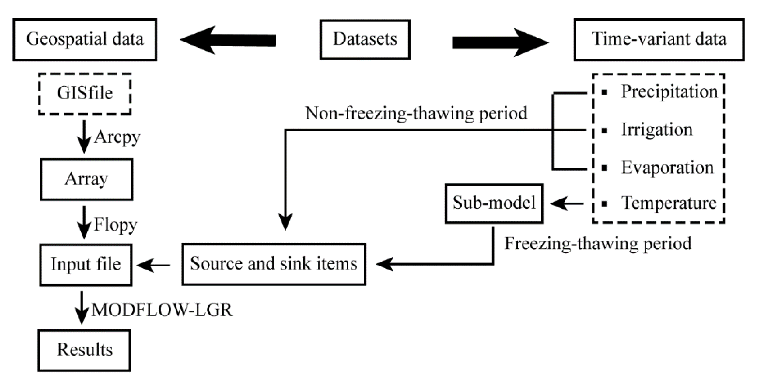
2.2.4. Flowchart of the Coupled Model

The flowchart of the coupled model is shown in Figure 4. The model processes the spatial information (raster files or shapefiles) as multi-dimensional arrays, which are used by Flopy [62] to prepare input files for MODFLOW-LGR model. The source and sink items are calculated by Equations (12)–(16) in the non-freezing-thawing period and Equation (6) in the freezing-thawing period. Then, the model runs MODFLOW-LGR to obtain the simulation results.

2.3. Calibration and Validation of the Empirical Mothod

The mean absolute error (MAE), relative root mean square error (RRMSE), percent bias (PBIAS) and correlation coefficient (R) are introduced as evaluation indexes for model performance, and the calculation formulas are as follows,

$$MAE=\frac{1}{m}{\displaystyle \sum _{i=1}^m\left|X_{cal,i}-X_{obs,i}\right|}$$

(17)

$$RRMSE=\sqrt{\frac{{\displaystyle \sum _{i=1}^m{\left(X_{cal,i}-X_{obs,i}\right)}^2}}{m{\left(\frac{1}{m}{\displaystyle \sum _{i=1}^m{X}_{obs,i}}\right)}^2}}$$

(18)

$$PBIAS=\frac{{\displaystyle \sum _{i=1}^m\left(X_{obs,i}-X_{cal,i}\right)}}{{\displaystyle \sum _{i=1}^m{X}_{obs,i}}}$$

(19)

$$R=\frac{{\displaystyle \sum _{i=1}^m\left(X_{obs,i}-\overline{X_{obs}}\right)\left(X_{cal,i}-\overline{X_{cal}}\right)}}{\sqrt{{\displaystyle \sum _{i=1}^m{\left(X_{obs,i}-\overline{X_{obs}}\right)}^2{\displaystyle \sum _{i=1}^m{\left(X_{cal,i}-\overline{X_{cal}}\right)}^2}}}}$$

(20)

where X_cal,i is the calculated value; X_obs,i is the observed value; m is the sample size.

The observed air temperature from five weather stations and the according water table depth during the freezing-thawing period in Hetao Irrigation District, Inner Mongolia, China were used to test the validity of the empirical method elaborated in Section 2.2.2. The locations of the weather stations are shown in Figure 1.

The parameters for fitting the temperature-time curve and water table depth-time curve shown in Equation (6) and (7) of the five sub-areas and the lagging days calculated by Equation (9) are listed in

Table 1. Parameters and model evaluation indexes of the sub-model applied in Hetao Irrigation District.

Sub-Irrigation District	[αT, βT, γT] (°C, –, °C)	[αH, βH, γH] (m, –, m)	Lagging Days (d)	MAE (m)	RRMSE (%)	PBIAS (%)	R
Ulanbuh	[16.07, 2.91, 9.56]	[−0.905, 2.162, −0.106]	43	0.105	6.53	−3.86	0.94
Jiefangzha	[15.74, 2.91, 8.38]	[−1.045, 2.045, −0.001]	50	0.123	7.35	−4.22	0.97
Yongji	[15.95, 2.91, 8.97]	[−0.817, 1.978, 0.035]	54	0.104	6.23	−2.93	0.93
Yichang	[16.34, 2.90, 8.21]	[−1.092, 2.087, −0.055]	47	0.158	9.56	−5.31	0.95
Urad	[16.23, 2.90, 9.34]	[−1.034, 2.232, −0.221]	39	0.173	11.46	−5.33	0.87

. Then, the water table depth during the freezing-thawing period can be calculated by using Equation (10). The calculated water table depths were compared with the observed values as shown in Figure 5, which showed a good agreement with the MAE values ranging from 0.104 m and 0.173 m, and the RRMSE values from 6.23% and 11.46%. Percent bias (PBIAS) measures the average tendency of the calculated data to be larger or smaller than their observed counterparts. The PBIAS values listed in Table 1 were smaller than ±10%, which indicates that the sub-model performance is very good. The correlation coefficients are from 0.87 to 0.97. These results demonstrate that the sub-model can accurately predict the water table depth during the freezing-thawing period, which can then be used to calculate the groundwater recharge/discharge during the freezing-thawing period by using Equation (11).

As shown in Figure 5, the calculated water table depth deviates more from the measured value when the initial water table depth of freezing-thawing period is deeper than 1.9 m. The MAE and RRMSE values of the calculated and observed water table depth were 0.115 m and 7.1% when the initial water table depth is shallower than 1.9 m, and 0.318 m and 15% when it is deeper than 1.9 m. The freezing and thawing process mainly depends on the soil temperature, which changes periodically with the air temperature. The influence of air temperature on soil temperature decreases with the increase in soil depth. Therefore, the sub-model is more suitable for areas with shallow groundwater.

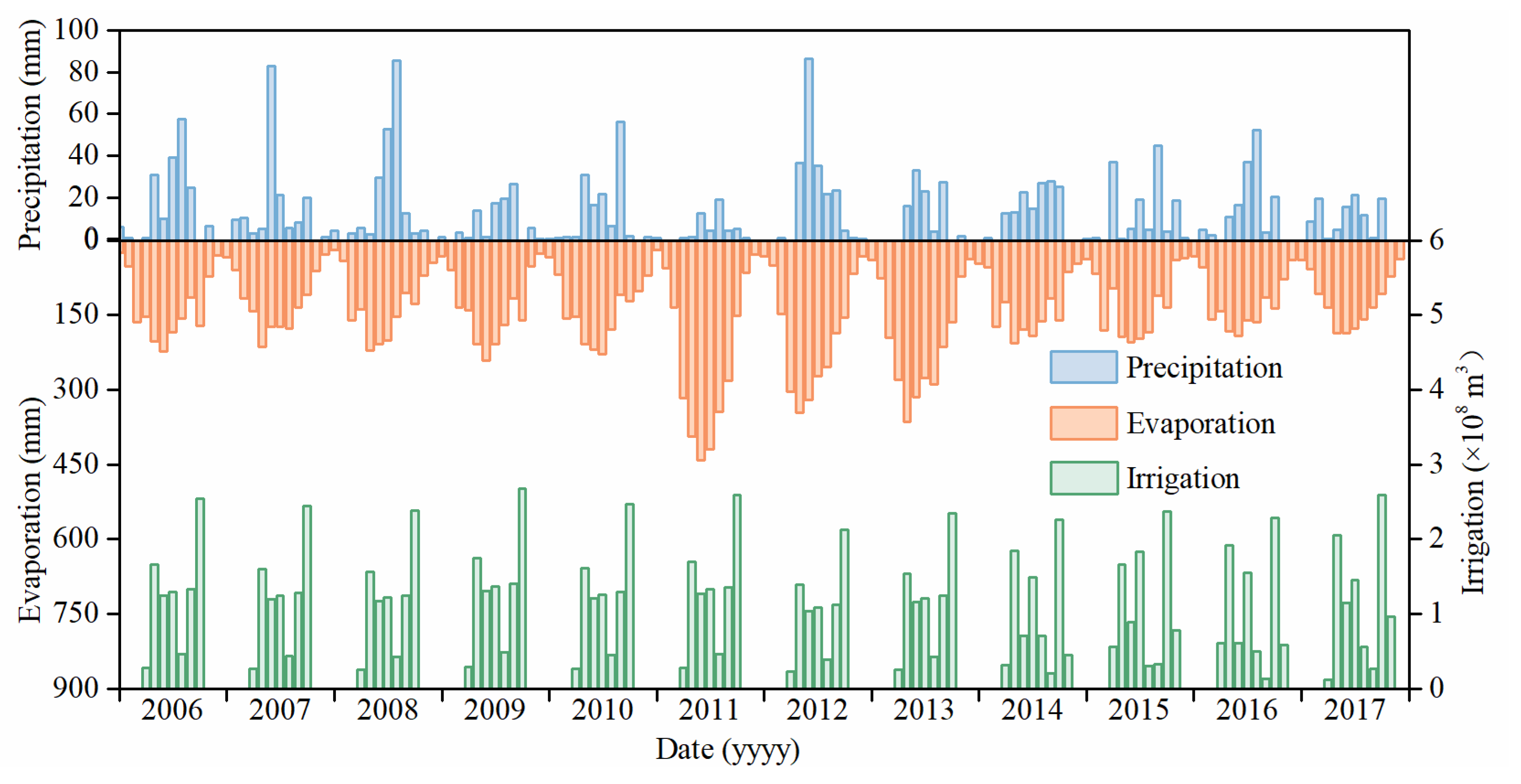
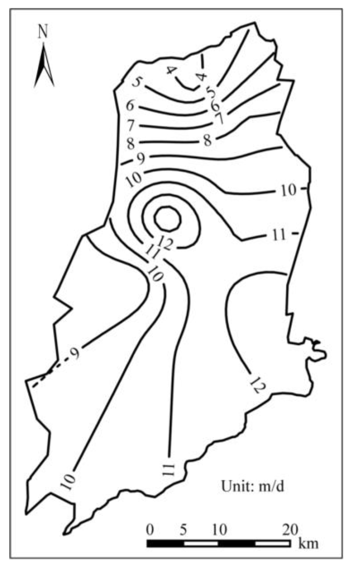
2.4. Data Preparation for the Study Area

The model mentioned above was used to investigate the groundwater exploitation scheme and calculate the relationship between the groundwater table depth and the layout parameters of the well-irrigated areas in the study area. Moreover, the groundwater in the study area flows from the south-west area with lower groundwater salinity to the north-east area with higher groundwater salinity area currently. Because of the plan of using groundwater for irrigation, the water table depth will be changed and the future groundwater flow should be investigated to avoid the salt water intrusion. Therefore, the validated MODFLOW-LGR model was used to evaluate the variation of the groundwater flow field. The measured data from 2006 to 2012 were used for model calibration, while the measured data from 2013 to 2017 were used for model validation. Then, different groundwater exploitation schemes were adopted to find the most suitable layout parameters of the well-irrigated areas, and the groundwater dynamics of Yongji sub-irrigation district after well-canal conjunctive irrigation was further predicted by the model.

In the horizontal direction, the parent model of the whole Yongji sub-irrigation district was discretized into a grid of 240 rows and 120 columns, with 28,800 grids, among which 14,406 were active grids. The horizontal grid size was set as 404.20 m in length and 344.50 m in width. The local grid refinement was used for Longsheng well-irrigated area and the ratio of refinement was 5:1 with the dimension of the child grids as 80.84 × 68.90 m. The child model was divided into 65 rows and 50 columns with a total of 3250 grids. The use of LGR removed 18,765 unnecessary refined grids compared with the traditional refinement method. The domain was divided into three layers in the vertical direction. The first layer was consistent with the less permeable layer, characterizing the upper unconfined aquifer. The lower, more permeable layer was divided into the second and third layers, representing the underlying semi-confined aquifer. The initial groundwater level was interpolated from the measured value of 1 January 2006 during the calibration period and 1 January 2013 during the validation period respectively. One natural month was regarded as a stress period, and the time step was set as 1 d.

The hydrogeological parameters required by the model include horizontal and vertical hydraulic conductivity, specific yield and specific storage of each layer. The horizontal hydraulic conductivity of the second and third layer was interpolated according to the results of pumping test as shown in Figure 6, ranging between 3.74 m/d and 13.89 m/d, and that of the first layer was determined by the model calibration. This area is formed by river accretion and the vertical hydraulic conductivity is much smaller than the horizontal hydraulic conductivity. The vertical hydraulic conductivity was set as 1/10 of the horizontal hydraulic conductivity for anisothropy simulation referred to previous research [63,64]. The soil is sandy loam in the south of the area because of the alluviation of the Yellow River and because the hydraulic conductivity is larger. The soil texture gradually becomes clayey from south to north, which is mixed with silt loam and clay and is less permeable [65,66]. The soil sand content is higher in local middle areas according to the results of pumping test, thus, the hydraulic conductivity is larger in the middle of the area, as Figure 6 shows. The specific yield of the first layer was determined by the model calibration. The specific storage of the second and third layers was set as 2 × 10⁻⁶ m⁻¹, which were obtained based on the previous hydrogeological studies.

The recharge from irrigation imposing on the upper boundary was categorized into 12 zones based on the controlling area of the main canals and drains. The monthly diversion water was used to calculate the net recharge for groundwater, and the recharge coefficient was obtained by calibration. The recharge coefficient from precipitation was set as 0.1 [67]. The two coefficients σ and ξ used for calculating the phreatic evaporation were determined by field trial [68,69]. The extinction depth was set as 4 m.

3. Results and Discussion

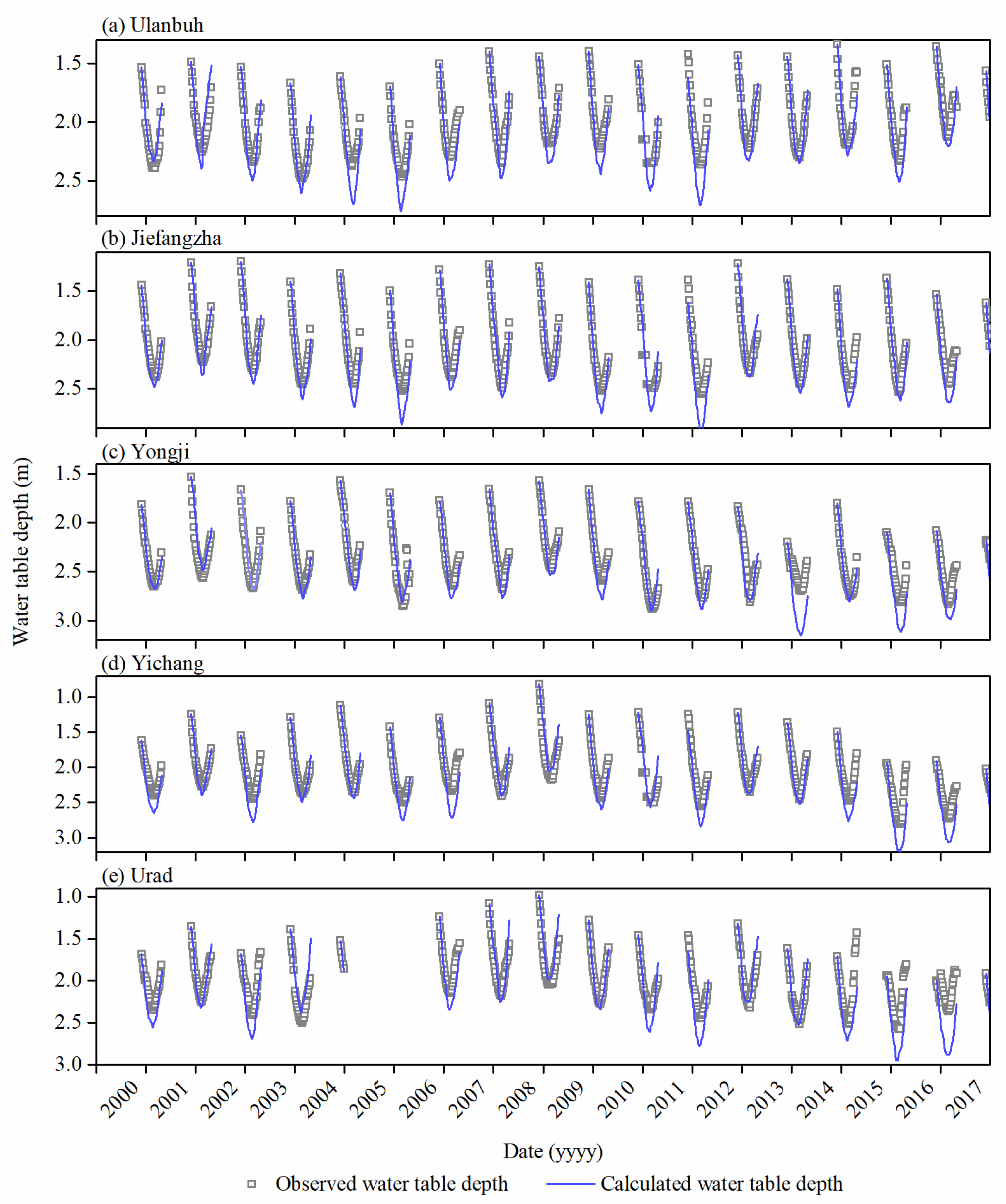
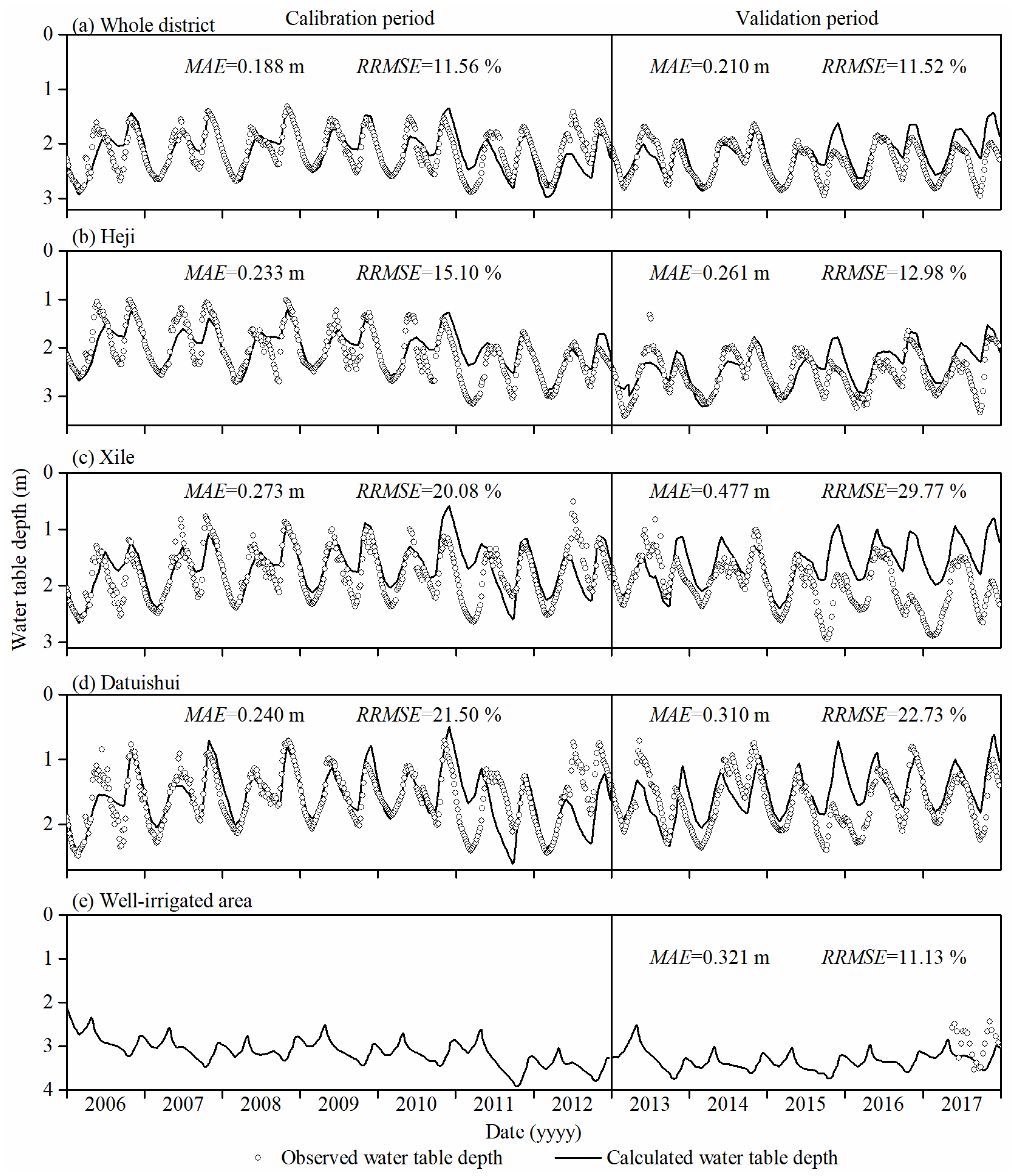
3.1. Calibration and Validation of MODFLOW-LGR

The calculated and observed water table depth of different areas in the calibration (2006–2012) and validation (2013–2017) periods are shown in Figure 7. The MAE values of water table depth averaging the whole domain were 0.188 m and 0.210 m, RRMSE values were 11.56% and 11.52% in the calibration and validation periods, respectively, which indicated that the model can reasonably simulate the water table depth. The model performances of different irrigation control areas were slightly different, with the MAE between 0.229 m and 0.481 m, and RRMSE between 7.59% and 37.33%. Overall, the simulation results of the calibration period were better than those of the validation period. Since the observation wells in the well-irrigated area were set from May 2017, only a short duration of comparison between the observed and calculated water table depth in the well-irrigated area is shown in Figure 7e. The MAE and RRMSE were 0.321 m and 11.13%.

The evaluation indexes of calculated and observed water table depth during the freezing-thawing periods from 2006 to 2017 are listed in

Table 2. Model evaluation indexes of calculated and observed water table depth during the freezing-thawing period.

Irrigation Area	MAE (m)	RRMSE (%)	PBIAS (%)	R
Whole district	0.151	8.38	3.23	0.84
Heji	0.181	10.56	4.56	0.84
Nanbian	0.387	21.88	11.40	0.37
Beibian	0.387	9.25	−5.06	0.58
Yonglan	0.214	12.84	3.49	0.84
Yonggang	0.253	13.79	−7.34	0.73
Xile	0.333	21.74	14.50	0.59
Xinhua	0.232	15.01	−1.29	0.72
Tiancai	0.344	27.59	−11.30	0.58
Xinji	0.243	19.14	−7.10	0.71
Datuishui	0.252	18.48	12.25	0.76
Zhengshao	0.355	19.28	12.41	0.64

. The MAE of different areas changed between 0.181 m and 0.387 m, and RRMSE between 9.25% and 27.59%. The MAE and RRMSE values of the whole district were 0.151 m and 8.38%, respectively. The PBIAS value was 3.23% and the correlation coefficient was 0.84 of the whole district, which demonstrated the accuracy of the groundwater recharge model during the freezing-thawing period.

The model parameters were calibrated including the specific yield and the horizontal hydraulic conductivity of the first layer and the recharge coefficient of irrigation water α_i. The specific yield and horizontal hydraulic conductivity of the first layer were set with an average value of 0.04 and 0.926 m/d. The calibrated α_i in the canal-irrigated area is shown in

Table 3. Calibration results of recharge coefficient of irrigation water in different areas and different periods.

Irrigation Area	Months
	Growth Period					Autumn Irrigation Period
	May	June	July	August	September	October	November
Heji	0.3	0.3	0.1	0.1	0.1	0.3	0.3
Nanbian	0.3	0.3	0.1	0.1	0.1	0.3	0.3
Beibian	0.35	0.35	0.2	0.2	0.2	0.35	0.35
Yonglan	0.35	0.35	0.1	0.1	0.1	0.3	0.3
Yonggang	0.35	0.35	0.1	0.1	0.1	0.3	0.3
Erhao	0.3	0.3	0.1	0.1	0.1	0.3	0.3
Xile	0.3	0.3	0.1	0.1	0.1	0.3	0.3
Xinhua	0.3	0.3	0.1	0.1	0.1	0.3	0.3
Tiancai	0.35	0.35	0.1	0.1	0.1	0.3	0.3
Xinji	0.35	0.35	0.15	0.15	0.15	0.35	0.35
Datuishui	0.3	0.3	0.1	0.1	0.1	0.3	0.3
Zhengshao	0.2	0.2	0.1	0.1	0.1	0.2	0.2

. The values were changed monthly due to the various growing stages of crops and the irrigation amount. In the early growth period (mid-May to late June), the recharge coefficient was larger due to the smaller water consumption of plants. In the late growth period (early July to mid-September), the crops grew vigorously and consumed a large amount of water, which resulted in a smaller recharge for groundwater. There was no crop growing in the autumn irrigation period and a large amount of water was applied, which caused a larger recharge coefficient ranging from 0.2 to 0.35. The α_i in the well-irrigated area during the growth period was 0.11. The recharge coefficient of irrigation in the well-irrigated area during the autumn irrigation period was set as the same as that in the canal-irrigated area.

3.2. Water Mass Balance and Exchange Between the Parent and Child Areas

The annual water balance data are listed in

Table 4. Annual average water balance items in the parent and child domains during the calibration and validation periods.

	Water Balance Items (×104 m3)	Calibration Period	Validation Period
Parent model domain (Yongji sub-irrigation district)	Recharge from irrigation and precipitation	15,226	14,926
	Recharge from river	6819	6404
	Phreatic evaporation	21,435	20,253
	Discharge to drains	206	233
Child model domain (Longsheng well-irrigated area)	Recharge from irrigation and precipitation	22	22
	Phreatic evaporation	58	45
	Discharge to drains	0	0
	Pumping water in the well-irrigated area	216	216
	Recharge from parent model	239	243

. The annual average amount of recharge from irrigation and precipitation to the aquifer was 15,226 × 10⁴ m³/y in the calibration period and 14,926 × 10⁴ m³/y in the validation period. The annual average river recharge to groundwater was 6819 × 10⁴ m³/y and 6404 × 10⁴ m³/y in the calibration and validation periods, respectively, which accounted for 44% of the total inflow. This budget illustrated the great importance of the Yellow River as a recharge source of the aquifer. The annual average phreatic evaporation from the groundwater was 21,435 × 10⁴ m³/y in the calibration period and 20,253 × 10⁴ m³/y in the validation period, which was the largest outflow of the aquifer. In the Longsheng well-irrigated area, the water table depth was deeper than that of the surrounding area, which resulted in the lateral recharge from the surrounding area to the well-irrigated area. The annual average lateral recharge was 239 × 10⁴ m³/y and 243 × 10⁴ m³/y in the calibration and validation periods, respectively, which were close to the amount of groundwater abstraction in the well-irrigated area 216 × 10⁴ m³/y. The equilibrium of the lateral recharge and the abstraction is important for avoiding a deep cone of depression.

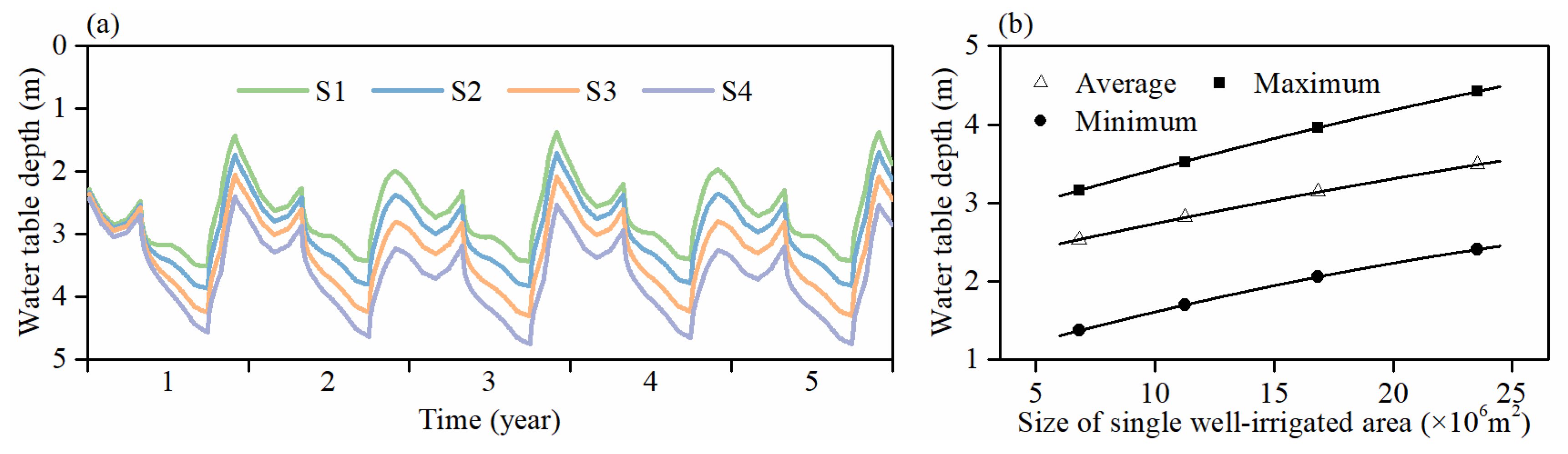
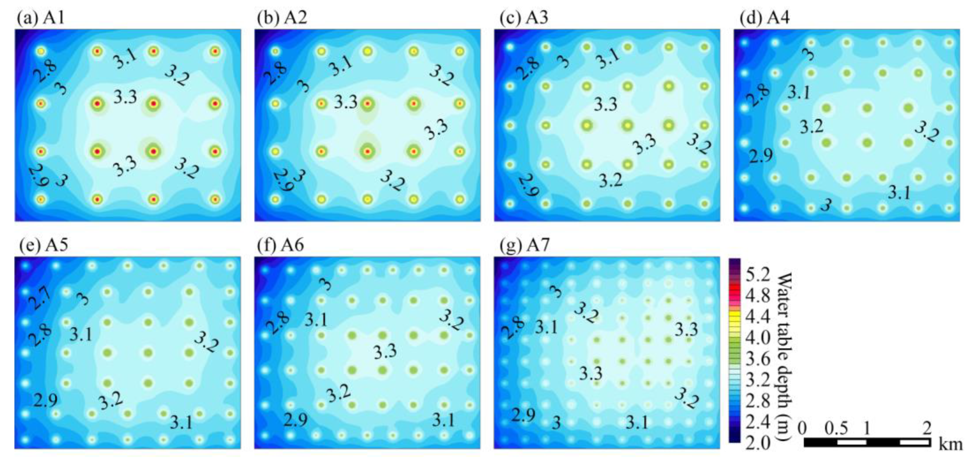
3.3. Model Application for Planning Suitable Size of Well-Irrigated Area

The lateral recharge from the surrounding canal-irrigated area is the major source for the well-irrigated area. It becomes more difficult to obtain recharge with a larger size of single well-irrigated area. The calibrated MODFLOW-LGR model was further used to predict the groundwater dynamics under 4 scenarios of well-irrigated area. The sizes of the 4 scenarios were 6.82 × 10⁶ m², 11.28 × 10⁶ m², 16.85 × 10⁶ m² and 23.54 × 10⁶ m², which were 75%, 125%, 186% and 260% of the size of Longsheng well-irrigated area, marked as S1, S2, S3, S4. There were 30, 50, 74, and 104 pumping wells uniformly distributed in the 4 scenarios of the well-irrigated area. The water table depths in the future 5 years after well-canal conjunctive irrigation under the 4 scenarios were predicted, as the spatial average water table depth shown in Figure 8a. The results showed that larger size of single well-irrigated area led to deeper water table depth. Figure 8b shows the relationship between the average, maximum and minimum water table depths and the size of single well-irrigated area. The average water table depths under the 4 scenarios were 2.68 m, 2.96 m, 3.30 m and 3.65 m. The suitable water table depth for natural vegetation and crop growth and soil salinization prevention in Hetao Irrigation District was 2–3 m [70,71]. As shown in Figure 8b, when the size of well-irrigated area was larger than 15 × 10⁶ m², the average water table depth was deeper than the suitable water table depth.

The water mass balance of well-irrigated area under four scenarios is shown in

Table 5. Annual average water balance of well-irrigated area of 4 scenarios with different size of single well-irrigated area.

Equilibrium (×104 m3)	S1	S2	S3	S4
Recharge from irrigation and precipitation	26.87	44.42	66.36	92.69
Phreatic evaporation	28.66	34.27	32.57	26.26
Discharge to drains	0	0	0	0
Pumping water in the well-irrigated area	145.18	240.13	358.70	501.12
Recharge from the surrounding canal-irrigated area	149.07	231.43	323.05	425.42
The ratio of recharge from canal-irrigated area to amount of pumping water (%)	103	96	90	85

. It demonstrated that more than 80% inflow of the aquifer came from the lateral recharge of the surrounding canal-irrigated area. However, with the increase in the well-irrigated area size, the proportion of the recharge from the canal-irrigated area to the amount of pumping water was getting smaller, which were 103%, 96%, 90% and 85% under the four scenarios. It indicated that the deviation between the lateral recharge and pumping water increased with the larger size of single well-irrigated area. The lateral recharge from the surrounding canal-irrigated area was larger than the pumping water under S1, which indicated that this scenario was too conservative. S2 and S3 were considered as the appropriated ones because of the equilibrium between the lateral recharge and pumping water in the well-irrigated area. The size of the well-irrigated area under S4 was too large to obtain abundant recharge for water usage in the well-irrigated area. Generally, by the comprehensive analysis of water table depth and the water balance, the suitable size of single well-irrigated area ranges between 11 × 10⁶ m² and 15 × 10⁶ m²

3.4. Model Application for Planning Suitable Controlling Irrigation Area of Single Well

In the case of a certain irrigation quota, more groundwater exploitation from each well is necessary with a larger controlling irrigation area of single well, which would result in the deeper water table depth around the pumping well. Based on the designed controlling irrigation area of 12 × 10⁴ m² of a single well in Longsheng well-irrigated area, seven scenarios of different controlling irrigation areas of single well were set, marked as A1–A7 shown in

Table 6. The maximum water table depth and area proportion with average water table depth exceeds 2.8 m under the seven scenarios with different controlling irrigation area of single well.

Scenario No.	Controlling Irrigation Area of Single Well (×104 m2)	Maximum Water Table Depth (m)	Percentage of Area with Average Water Table Depth Exceeds 2.8 m (%)
A1	45.97	6.37	61.58
A2	36.77	5.90	61.14
A3	24.52	5.16	61.14
A4	18.39	4.72	59.01
A5	16.34	4.59	56.99
A6	14.71	4.55	60.64
A7	7.35	4.17	60.69

. The average water table depth of the well-irrigated area under the seven scenarios was close, with an average of 2.8 m. The maximum water table depth varied greatly among different scenarios, ranging from 4.17 m to 6.37 m. The percentages of area with average water table depth deeper than 2.8 m are also listed in Table 6. The percentage value decreased from 61.58% to 56.99% when the controlling irrigation area of single well changed from 45.97 × 10⁴ m² (A1) to 16.34 × 10⁴ m² (A5), while the value increased from 56.99% to 60.69% when the controlling irrigation area of single well changed from 16.34 × 10⁴ m² (A5) to 7.35 × 10⁴ m² (A7). The spatial distribution of average water table depth during the crop growth period under the seven scenarios is shown in Figure 9. A larger pumping water amount of single well resulted in deeper depression cones and a wider influence range as shown in Figure 9a. However, the controlling irrigation area of single well should not be too small. Although there were no deep cones of depression with the smallest area of single well as shown in Figure 9g, the superposition effect of groundwater drawdown would cause a larger area with the average water table depth deeper than 2.8 m. Therefore, the controlling irrigation area of single well should neither be too large nor too small, and the recommended area was 15 × 10⁴ m²–19 × 10⁴ m².

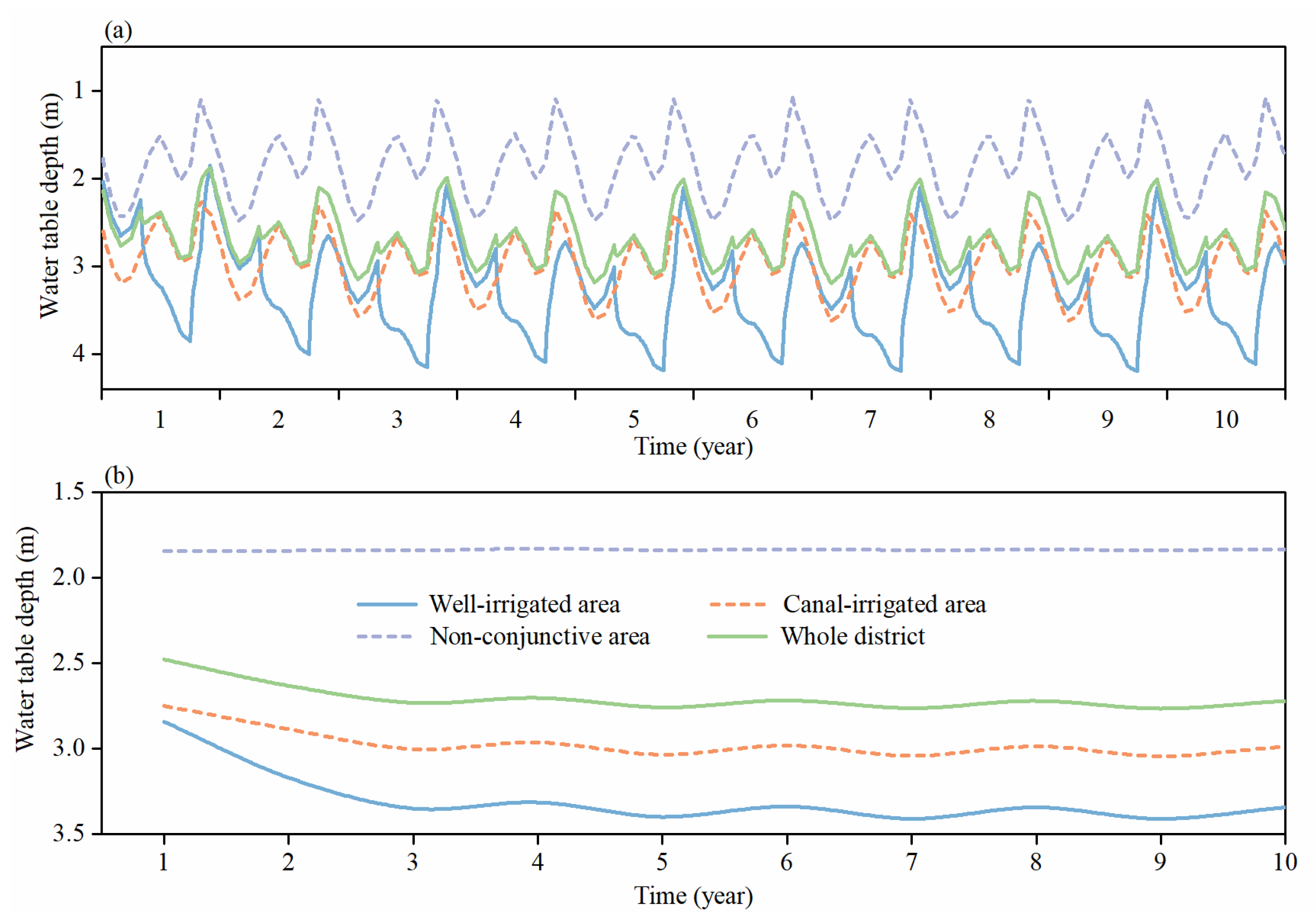
3.5. Groundwater Dynamics Prediction in Yongji Sub-Irrigation District under the Well-Canal Conjunctive Irrigation Plan

The recommended layout parameters of well-irrigated area obtained above were adopted to plan the well-canal irrigation scheme in Yongji sub-irrigation district. There will be 16 well-irrigated areas planned in Yongji sub-irrigation district as shown in Figure 10a, with the size of single well-irrigated area 11.28 × 10⁶ m², and the controlling irrigation area of single well 16.34 × 10⁴ m². The pumping wells were uniformly arranged as shown in Figure 10b. The calibrated MODFLOW-LGR was then used to predict the groundwater dynamics under this planned well-canal irrigation scheme. The local refinement grids were applied in each well-irrigated area with 16 child models. Figure 11a shows the changes in water table depth in different regions after well-canal conjunctive irrigation, and the annual average water table depths of different regions are shown in Figure 11b. The increase in water table depth can be found after conjunctive use of well-canal irrigation. The spatial distribution of water table depth during the growth period of the whole irrigation district and one well-irrigated area (No. 9) are shown in Figure 10c,d. The deeper water table depth can be found in the south of Yongji sub-irrigation district, and cones of depression appear around well-irrigated area as shown in Figure 10c,d, further illustrating the water table depth in a typical well-irrigated area and the details of depression cones around wells. In total, the average water table depth is 3.29 m in the well-irrigated area, 2.97 m in the canal-irrigated area, 1.84 m in the non-conjunctive area and 2.7 m in the whole irrigation district after the well-canal conjunctive irrigation. From the point of controlling water table depth, the proposed layout scheme is feasible for Yongji sub-irrigation district.

The water mass balance of each well-irrigated area is listed in

Table 7. Annual average water balance of different areas after well-canal conjunctive irrigation.

No.	Equilibrium (×104 m3)
	Recharge from Irrigation and Precipitation	Phreatic Evaporation	Pumping Water in the Well-irrigated Area	Recharge from Canal-Irrigated Area
1	39.24	32.81	240.13	228.00
2	39.24	23.29	240.13	217.00
3	39.24	21.42	240.13	214.92
4	39.24	19.60	240.13	215.55
5	39.24	8.31	240.13	201.30
6	39.24	11.26	240.13	206.37
7	39.24	17.18	240.13	214.32
8	39.24	30.22	240.13	225.53
9	39.24	25.21	240.13	223.45
10	39.24	39.11	240.13	237.63
11	39.24	55.06	240.13	253.61
12	39.24	16.49	240.13	215.79
13	39.24	55.18	240.13	252.41
14	39.24	29.90	240.13	228.73
15	39.24	5.25	240.13	200.36
16	39.24	33.62	240.13	231.18
Well-irrigated area	628	424	3842	3566

. The recharge from the surrounding canal-irrigated area ranged from 200.36 × 10⁴ m³/y to 253.61 × 10⁴ m³/y. There was 3842 × 10⁴ m³/y of groundwater extracted and used in the well-irrigated areas. The recharge from the surrounding canal-irrigated area to the well-irrigated area was 3566 × 10⁴ m³/y, accounting for 93% of pumping water used in the well-irrigated areas. The adequate lateral recharge ensures the sustainability of the abstraction groundwater in well-irrigated areas.

4. Conclusions

This study presented a sub-model to calculate the recharge/discharge of groundwater system in the freezing-thawing period and integrated the sub-model with the multiscale groundwater model MODFLOW-LGR for the whole year groundwater simulation. The model was then applied to estimate the suitable layout parameters of a well-irrigated area, including the size of the well-irrigated area and the irrigation area of single well. A well-canal conjunctive irrigation scheme was finally put forward in Yongji sub-irrigation district, which can ensure the adequate lateral recharge from canal-irrigated areas to well-irrigated areas and maintain reasonable water table depth. The major conclusions are as follows.

Temperature is effective to be used to estimate the groundwater recharge/discharge during the freezing-thawing period in agricultural areas with shallow water table depth.

The MODFLOW-LGR model with the sub-model to calculate the recharge/discharge of groundwater system in the freezing-thawing period is accurate for groundwater prediction in seasonal freezing-thawing areas.

The local grid refinement method reduces the unnecessary refined grids and performs well in evaluating groundwater exchange along the interface of parent and child models, which is necessary and important to estimate the lateral recharge from canal-irrigated areas to well-irrigated areas.

The recommended size of a single well-irrigated area in Yongji Irrigation District ranges from 11 × 10⁶ m² to 15 × 10⁶ m², and the controlling irrigation area of single well is 15 × 10⁴ m² to 19 × 10⁴ m².

References

1. Bamberger, M.; Johnson, P.L. Methodology of the world development report 1992: Development and the environment. Eval. Pract. 1993, 14, 275–287. [Google Scholar] [CrossRef]
2. Mariolakos, I. Water resources management in the framework of sustainable development. Desalination 2007, 213, 147–151. [Google Scholar] [CrossRef]
3. Fasakhodi, A.A.; Nouri, S.H.; Amini, M. Water Resources Sustainability and optimal cropping pattern in farming systems; a multi-objective fractional goal programming approach. Water Resour. Manag. 2010, 24, 4639–4657. [Google Scholar] [CrossRef]
4. Van Dam, J.C.; Singh, R.; Bessembinder, J.J.E.; Leffelaar, P.A.; Bastiaanssen, W.G.M.; Jhorar, R.K.; Kroes, J.G.; Droogers, P. Assessing options to increase water productivity in irrigated river basins using remote sensing and modelling tools. Water Resour. Dev. 2006, 22, 115–133. [Google Scholar] [CrossRef]
5. Singh, A. Conjunctive use of water resources for sustainable irrigated agriculture. J. Hydrol. 2014, 519, 1688–1697. [Google Scholar] [CrossRef]
6. Mao, W.; Yang, J.Z.; Zhu, Y.; Ye, M.; Wu, J.W. Loosely coupled SaltMod for simulating groundwater and salt dynamics under well-canal conjunctive irrigation in semi-arid areas. Agr. Water Manag. 2017, 192, 209–220. [Google Scholar] [CrossRef]
7. Chang, L.C.; Ho, C.C.; Yeh, M.S.; Yang, C.C. An integrating approach for conjunctive-use planning of surface and subsurface water system. Water Resour. Manag. 2011, 25, 59–78. [Google Scholar] [CrossRef]
8. Cheng, Y.; Lee, C.H.; Tan, Y.C.; Yeh, H.F. An optimal water allocation for an irrigation district in Pingtung County, Taiwan. Irrig. Drain. 2009, 58, 287–306. [Google Scholar] [CrossRef]
9. Cosgrove, D.M.; Johnson, G.S. Aquifer management zones based on simulated surface-water response functions. J. Water Resour. Plan. Manag. 2005, 131, 89–100. [Google Scholar] [CrossRef]
10. Fisher, A.; Fullerton, D.; Hatch, N.; Reinelt, P. Alternatives for managing drought: A comparative cost analysis. J. Environ. Econ. Manag. 1995, 29, 304–320. [Google Scholar] [CrossRef] [Green Version]
11. Mani, A.; Tsai, F.T.C.; Kao, S.C.; Naz, B.S.; Ashfaq, M.; Rastogi, D. Conjunctive management of surface and groundwater resources under projected future climate change scenarios. J. Hydrol. 2016, 540, 397–411. [Google Scholar] [CrossRef] [Green Version]
12. Zhang, X.D. Conjunctive surface water and groundwater management under climate change. Front. Environ. Sci. 2015, 3, 1–10. [Google Scholar] [CrossRef]
13. Ejaz, M.S.; Peralta, R.C. Maximizing conjunctive use of surface and ground water under surface water quality constraints. Adv. Water Resour. 1995, 18, 67–75. [Google Scholar] [CrossRef] [Green Version]
14. Liu, L.G.; Cui, Y.L.; Luo, Y.F. Integrated modeling of conjunctive water use in a canal-well irrigation district in the lower Yellow River Basin, China. J. Irrig. Drain. Eng. 2013, 139, 775–784. [Google Scholar] [CrossRef]
15. Azaiez, M.N. A model for conjunctive use of ground and surface water with opportunity costs. Eur. J. Oper. Res. 2002, 143, 611–624. [Google Scholar] [CrossRef]
16. Li, P.Y.; Qian, H.; Wu, J.H. Conjunctive use of groundwater and surface water to reduce soil salinization in the Yinchuan Plain, North-West China. Int. J. Water Resour. Dev. 2018, 34, 337–353. [Google Scholar] [CrossRef]
17. Surapaneni, A.; Olsson, K.A. Sodification under conjunctive water use in the Shepparton Irrigation Region of northern Victoria: A review. Aust. J. Exp. Agric. 2002, 42, 249–263. [Google Scholar] [CrossRef]
18. Gleeson, T.; VanderSteen, J.; Sophocleous, M.A.; Taniguchi, M.; Alley, W.M.; Allen, D.M.; Zhou, Y. Groundwater sustainability strategies. Nat. Geosci. 2010, 3, 378–379. [Google Scholar] [CrossRef]
19. Tilman, D.; Cassman, K.G.; Matson, P.A.; Naylor, R.; Polasky, S. Agricultural sustainability and intensive production practices. Nature 2002, 418, 671–677. [Google Scholar] [CrossRef]
20. Mao, W.; Yang, J.Z.; Zhu, Y.; Wu, J.W. Soil salinity process of Hetao Irrigation District after application of well-canal conjunctive irrigation and mulched drip irrigation. Trans. CSAE 2018, 34, 93–101. (In Chinese) [Google Scholar] [CrossRef]
21. Wu, J.W.; Yang, Y.; Zhu, Y.; Yu, L.S.; Yang, W.Y.; Yang, J.Z. Simulation and prediction of groundwater considering seasonal freezing-thawing in irrigation area with conjunctive use of groundwater and surface water. Trans. CSAE 2018, 34, 168–178. (In Chinese) [Google Scholar] [CrossRef]
22. Bejranonda, W.; Koch, M.; Koontanakulvong, S. Surface water and groundwater dynamic interaction models as guiding tools for optimal conjunctive water use policies in the central plain of Thailand. Environ. Earth Sci. 2013, 70, 2079–2086. [Google Scholar] [CrossRef]
23. El-Rawy, M.; Zlotnik, V.A.; Al-Raggad, M.; Al-Maktoumi, A.; Kacimov, A.; Abdalla, O. Conjunctive use of groundwater and surface water resources with aquifer recharge by treated wastewater: Evaluation of management scenarios in the Zarqa River Basin, Jordan. Environ. Earth Sci. 2016, 75, 1146.1–1146.21. [Google Scholar] [CrossRef]
24. Li, P.; Qi, X.B.; Nurolla, M.; Huang, Z.D.; Liang, Z.J.; Qiao, D.M. Response of precipitation to ratio of canal to wells and its environmental effects analysis in combined well-canal irrigation area. Trans. CSAE 2015, 31, 123–128. (In Chinese) [Google Scholar] [CrossRef]
25. Li, Z.; Quan, J.; Li, X.Y.; Wu, X.C.; Wu, H.W.; Li, Y.T.; Li, G.Y. Establishing a model of conjunctive regulation of surface water and groundwater in the arid regions. ” Agric. Water Manag. 2016, 174, 30–38. [Google Scholar] [CrossRef]
26. Seo, S.B.; Mahinthakumar, G.; Sankarasubramanian, A.; Kumar, M. Conjunctive management of surface water and groundwater resources under drought conditions using a fully coupled hydrological model. J. Water Resour. Plan. Manag. 2018, 144, 04018060.1–04018060.11. [Google Scholar] [CrossRef] [Green Version]
27. Ayvaz, M.T.; Karahan, H. A simulation/optimization model for the identification of unknown groundwater well locations and pumping rates. J. Hydrol. 2008, 357, 76–92. [Google Scholar] [CrossRef]
28. Bayer, P.; Duran, E.; Baumann, R.; Finkel, M. Optimized groundwater drawdown in a subsiding urban mining area. J. Hydrol. 2009, 365, 95–104. [Google Scholar] [CrossRef]
29. Huang, C.; Mayer, A.S. Pump-and-treat optimization using well locations and pumping rates as decision variables. Water Resour. Res. 1997, 33, 1001–1012. [Google Scholar] [CrossRef]
30. Katsifarakis, K.L.; Nikoletos, I.A.; Stavridis, C. Minimization of transient groundwater pumping cost-analytical and practical solutions. Water Resour. Manag. 2018, 32, 1053–1069. [Google Scholar] [CrossRef]
31. Moreno, M.A.; Córcoles, J.I.; Moraleda, D.A.; Martinez, A.; Tarjuelo, J.M. Optimization of underground water pumping. J. Irrig. Drain. Eng. 2010, 136, 414–420. [Google Scholar] [CrossRef]
32. Park, C.H.; Aral, M.M. Multi-objective optimization of pumping rates and well placement in coastal aquifers. J. Hydrol. 2004, 290, 80–99. [Google Scholar] [CrossRef]
33. Lee, H.; Koo, M.H.; Oh, S. Modeling stream-aquifer interactions under seasonal groundwater pumping and managed aquifer recharge. Groundwater 2019, 57, 216–225. [Google Scholar] [CrossRef] [PubMed]
34. Mikita, M.; Yamanaka, T.; Lorphensri, O. Anthropogenic changes in a confined groundwater flow system in the Bangkok basin, Thailand, part I: Was groundwater-recharge enhanced? Hydrol. Process. 2011, 25, 2726–2733. [Google Scholar] [CrossRef]
35. Mohanty, S.; Jha, M.K.; Kumar, A.; Brahmanand, P.S. Optimal development of groundwater in a well command of eastern India using integrated simulation and optimization modelling. Irrig. Drain. 2013, 62, 363–376. [Google Scholar] [CrossRef]
36. Sarwar, A.; Eggers, H. Development of a conjunctive use model to evaluate alternative management options for surface and groundwater resources. Hydrogeol. J. 2006, 14, 1676–1687. [Google Scholar] [CrossRef]
37. Seo, S.B.; Mahinthakumar, G.; Sankarasubramanian, A.; Kumar, M. Assessing the restoration time of surface water and groundwater systems under groundwater pumping. Stoch. Environ. Res. Risk Assess. 2018, 32, 2741–2759. [Google Scholar] [CrossRef]
38. Zume, J.; Tarhule, A. Simulating the impacts of groundwater pumping on stream–aquifer dynamics in semi-arid north-western Oklahoma, USA. Hydrogeol. J. 2008, 16, 797–810. [Google Scholar] [CrossRef]
39. Al-Salamah, I.S.; Ghazaw, Y.M.; Ghumman, A.R. Groundwater modeling of Saq Aquifer Buraydah Al Qassim for better water management strategies. Environ. Monit. Assess. 2011, 173, 851–860. [Google Scholar] [CrossRef]
40. Liu, C.W.; Lin, C.N.; Jang, C.H.; Chen, C.P.; Chang, J.F.; Fan, C.C.; Lou, K.H. Sustainable groundwater management in Kinmen Island. Hydrol. Process. 2006, 20, 4363–4372. [Google Scholar] [CrossRef]
41. McCallum, A.M.; Andersen, M.S.; Giambastiani, B.; Kelly, B.F.; Ian Acworth, R. River–aquifer interactions in a semi-arid environment stressed by groundwater abstraction. Hydrol. Process. 2013, 27, 1072–1085. [Google Scholar] [CrossRef]
42. Pokhrel, Y.N.; Koirala, S.; Yeh, P.J.F.; Hanasaki, N.; Longuevergne, L.; Kanae, S.; Oki, T. Incorporation of groundwater pumping in a global land surface model with the representation of human impacts. Water Resour. Res. 2015, 51, 78–96. [Google Scholar] [CrossRef] [Green Version]
43. Reshmidevi, T.V.; Kumar, D.N. Modelling the impact of extensive irrigation on the groundwater resources. Hydrol. Process. 2014, 28, 628–639. [Google Scholar] [CrossRef]
44. Mehl, S.; Hill, M.C.; Leake, S.A. Comparison of local grid refinement methods for MODFLOW. Groundwater 2006, 44, 792–796. [Google Scholar] [CrossRef] [PubMed]
45. Mehl, S.; Hill, M.C. Development and evaluation of a local grid refinement method for block-centered finite-difference groundwater models using shared nodes. Adv. Water Resour. 2002, 25, 497–511. [Google Scholar] [CrossRef]
46. Dickinson, J.E.; James, S.C.; Mehl, S.; Hill, M.C.; Leake, S.A.; Zyvoloski, G.A.; Faunt, C.C.; Eddebbarh, A.A. A new ghost-node method for linking different models and initial investigations of heterogeneity and nonmatching grids. Adv. Water Resour. 2007, 30, 1722–1736. [Google Scholar] [CrossRef]
47. Wu, M.S.; Huang, J.S.; Wu, J.W.; Tan, X.; Jansson, P.E. Experimental study on evaporation from seasonally frozen soils under various water, solute and groundwater conditions in Inner Mongolia, China. J. Hydrol. 2016, 535, 46–53. [Google Scholar] [CrossRef]
48. Li, R.P.; Shi, H.B.; Flerchinger, G.N.; Akae, T.; Wang, C.S. Simulation of freezing and thawing soils in Inner Mongolia Hetao Irrigation District, China. Geoderma 2012, 173–174, 28–33. [Google Scholar] [CrossRef]
49. Walvoord, M.A.; Kurylyk, B.L. Hydrologic impacts of thawing permafrost-a review. Vadose Zone J. 2016, 15. [Google Scholar] [CrossRef]
50. Booij, M.; Leijnse, A.; Haldorsen, S.; Heim, M.; Rueslåtten, H. Subpermafrost ground modeling in Ny-Ålesund, Svalbard. Nordic Hydrol. 1998, 29, 358–396. [Google Scholar] [CrossRef] [Green Version]
51. Frederick, J.M.; Buffett, B.A. Taliks in relict submarine permafrost and methane hydrate deposits: Pathways for gas escape under present and future conditions. J. Geophys. Res. Earth Sur. 2014, 119, 106–122. [Google Scholar] [CrossRef]
52. Grenier, C.; Anbergen, H.; Bense, V.; Chanzy, Q.; Coon, E.; Collier, N.; Costard, F.; Ferry, M.; Frampton, A.; Frederick, J.; et al. Groundwater flow and heat transport for systems undergoing freeze-thaw: Intercomparison of numerical simulators for 2D test cases. Adv. Water Resour. 2018, 114, 196–218. [Google Scholar] [CrossRef]
53. Shojae-Ghias, M.; Therrien, R.; Molson, J.; Lemieux, J.-M. Controls on permafrost thaw in a coupled groundwater flow and heat transport system: Iqaluit Airport, Nunavut, Canada. Hydrogeol. J. 2017, 25, 657–673. [Google Scholar] [CrossRef]
54. Hansson, K.; Šimůnek, J.; Mizoguchi, M.; Lundin, L.C.; van Genuchten, M.T. Water flow and heat transport in frozen soil: Numerical solution and freeze-thaw applications. Vadose Zone J. 2004, 3, 693–704. [Google Scholar] [CrossRef] [Green Version]
55. Assefa, K.A.; Woodbury, A.D. Transient, spatially varied groundwater recharge modeling. Water Resour. Res. 2013, 49, 4593–4606. [Google Scholar] [CrossRef]
56. Yang, W.Y.; Hao, P.J.; Zhu, Y.; Liu, J.S.; Yu, J.; Yang, J.Z. Groundwater dynamics forecast under conjunctive use of groundwater and surface water in seasonal freezing and thawing area. Trans. CSAE 2017, 33, 137–145. (In Chinese) [Google Scholar] [CrossRef]
57. Wang, L.Y.; Peng, P.Y.; Hao, P.J.; Yu, J.; Yang, J.Z.; Zhu, Y. Well-canal conjunctive irrigation mode and potential of water-saving amount based on the balance of exploitation and supplement for Hetao Irrigation District. China Rural Water Hydropower 2016, 8, 18–24. (In Chinese) [Google Scholar]
58. Mehl, S.W.; Hill, M.C. MODFLOW–LGR—Documentation of ghost node local grid refinement (LGR2) for multiple areas and the boundary flow and head (BFH2) package. In U.S. Geological Survey Techniques and Methods; Book 6, Chapter A44; USGS Publications: Reston, VA, USA, 2013; p. 43. Available online: https://pubs.usgs.gov/tm/6a44/pdf/T&M6A-44.pdf (accessed on 16 May 2021).
59. Cui, L.H.; Zhu, Y.; Zhao, T.X.; Ye, M.; Yang, J.Z.; Wu, J.W. Evaluation of upward flow of groundwater to freezing soils and rational per-freezing water table depth in agricultural areas. J. Hydrol. 2020, 585, 124825. [Google Scholar] [CrossRef]
60. Chen, J.F.; Zheng, X.Q.; Zhang, Y.B.; Qin, Z.D.; Sun, M. Simulation of soil moisture evaporation under different groundwater level depths during seasonal freeze-thaw period. Trans. Chin. Soc. Agric. Mach. 2015, 46, 131–140. (In Chinese) [Google Scholar]
61. Shang, S.H.; Lei, Z.D.; Yang, S.X.; Wang, Y.; Zhao, D.M. Study on soil water movement with changeable groundwater level during soil freezing and thawing. Trans. CSAE 1999, 15, 64–68. (In Chinese) [Google Scholar]
62. Bakker, M.; Post, V.; Langevin, C.D.; Hughes, J.D.; White, J.T.; Starn, J.J.; Fienen, M.N. Scripting MODFLOW model development using Python and Flopy. Groundwater 2016, 54, 733–739. [Google Scholar] [CrossRef]
63. Yang, W.Y. Numerical Simulation of Conjunctive Use of Groundwater and Surface Water in Yongji Irrigation Field of Hetao Irrigation District; Wuhan University: Wuhan, China, 2016. (In Chinese) [Google Scholar]
64. Yu, L.S. Numerical Simulation of Conjunctive Use of Groundwater and Surface Water in Hetao Irrigation District and Water Resources Forecast; Wuhan University: Wuhan, China, 2017. (In Chinese) [Google Scholar]
65. Sun, G.F. Study on Soil Salinity Dynamics at Multiple Scales and Long-Term Solute Balance Models in Arid Area; Wuhan University: Wuhan, China, 2020. (In Chinese) [Google Scholar]
66. Xu, X.; Huang, G.; Zhan, H.; Qu, Z.; Huang, Q. Integration of SWAP and MODFLOW-2000 for modeling groundwater dynamics in shallow water table areas. J. Hydrol. 2012, 412–413, 170–181. [Google Scholar] [CrossRef]
67. Huang, Y.; Hu, T.S.; Fan, X.L. Numerical simulation of groundwater in Yongji Irrigation Area in Hetao Irrigation District. China Rural Water Hydropower 2010, 2, 79–83. (In Chinese) [Google Scholar]
68. Qian, Y.P.; Wang, L.; Li, W.Y.; Lin, Y.P. Study on surface evaporation of Bayangaole experimental station. Hydrology 1998, 4, 35–38. (In Chinese) [Google Scholar]
69. Wang, Y.D. Analysis on changes of groundwater table before and after water saving reconstruction in Hetao Irrigation District. Water Sav. Irrig. 2002, 1, 15–17. (In Chinese) [Google Scholar]
70. Cui, Y.L.; Shao, J.L.; Han, S.P. Ecological environment adjustment by groundwater in northwest China. Earth Sci. Front. 2001, 8, 191–196. (In Chinese) [Google Scholar] [CrossRef]
71. Yang, L.H.; Shen, R.K.; Cao, X.L. Scheme of groundwater use in Hetao Irrigation District in Inner Mongolia. Trans. CSAE 2003, 19, 56–59. (In Chinese) [Google Scholar]
Figure 1. Geographic location of (a) Hetao Irrigation District, (b) Yongji sub-irrigation district and (c) Longsheng well-irrigated area.
Water 13 01384 g001
Figure 2. Monthly precipitation, evaporation and irrigation data of Yongji sub-irrigation district during 2006–2017.
Water 13 01384 g002
Figure 3. (a) The coupling scheme of parent model with the child model in MODFLOW-LGR, (b) daily temperature and water table depth in Hetao Irrigation District during the freezing-thawing period, and (c) schematic of phase difference between temperature and water table depth in a freezing-thawing period.
Water 13 01384 g003aWater 13 01384 g003b
Figure 4. Flowchart of coupled model.
Water 13 01384 g004
Figure 5. Comparison of calculated and observed water table depth in the freezing-thawing period in (a) Ulanbuh sub-irrigation district, (b) Jiefangzha sub-irrigation district, (c) Yongji sub-irrigation district, (d) Yichang sub-irrigation district, and (e) Urad sub-irrigation district.
Water 13 01384 g005
Figure 6. The measured horizontal hydraulic conductivity of the second and third layer.
Water 13 01384 g006
Figure 7. Comparison results of calculated and observed water table depth during the calibration and validation periods in (a) the whole district, (b) Heji sub-irrigation district, (c) Xile sub-irrigation district, (d) Datuishui sub-irrigation district and (e) the well-irrigated area.
Water 13 01384 g007
Figure 8. Predicted water table depth under the 4 scenarios with different size of single well-irrigated area, (a) the spatial average water table depth under the 4 scenarios in the future 5 years, and (b) the relationship between the water table depth and the size of single well-irrigated area.
Water 13 01384 g008
Figure 9. Spatial distribution of average water table depth during the growth period under (a) Scenario A1, (b) Scenario A2, (c) Scenario A3, (d) Scenario A4, (e) Scenario A5, (f) Scenario A6, (g) Scenario A7 with different controlling irrigation area of single well.
Water 13 01384 g009
Figure 10. The predicted water table depth in Yongji sub-irrigation district after well-canal conjunctive irrigation, (a) layout scheme of well-irrigated areas, (b) pumping wells in a well-irrigated area, (c) spatial distribution of water table depth during the growth period of Yongji sub-irrigation district under the well-canal conjunctive irrigation, and (d) spatial distribution of water table depth during the growth period of one well-irrigated area.
Water 13 01384 g010
Figure 11. (a) Predicted spatial average daily water table depths of different areas in the future 10 years after well-canal conjunctive irrigation, and (b) spatial average annual water table depths of different areas in the future 10 years after well-canal conjunctive irrigation.
Water 13 01384 g011