
The Impact of the Uncertain Input Data of Multi-Purpose Reservoir Volumes under Hydrological Extremes


Institute of Landscape Water Management, Faculty of Civil Engineering, Brno University of Technology, 602 00 Brno, Czech Republic
*
Author to whom correspondence should be addressed.
Water 2021, 13(10), 1389; https://doi.org/10.3390/w13101389
Submission received: 30 March 2021
/
Revised: 6 May 2021
/
Accepted: 12 May 2021
/
Published: 16 May 2021
(This article belongs to the Special Issue Hydrological Extremes in a Warming Climate: Nonstationarity, Uncertainties and Impacts)
Abstract
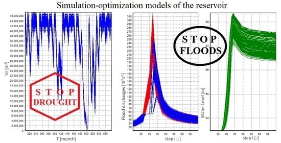
:The topic of uncertainties in water management tasks is a very extensive and highly discussed one. It is generally based on the theory that uncertainties comprise epistemic uncertainty and aleatoric uncertainty. This work deals with the comprehensive determination of the functional water volumes of a reservoir during extreme hydrological events under conditions of aleatoric uncertainty described as input data uncertainties. In this case, the input data uncertainties were constructed using the Monte Carlo method and applied to the data employed in the water management solution of the reservoir: (i) average monthly water inflows, (ii) hydrographs, (iii) bathygraphic curves and (iv) water losses by evaporation and dam seepage. To determine the storage volume of the reservoir, a simulation-optimization model of the reservoir was developed, which uses the balance equation of the reservoir to determine its optimal storage volume. For the second hydrological extreme, a simulation model for the transformation of flood discharges was developed, which works on the principle of the first order of the reservoir differential equation. By linking the two models, it is possible to comprehensively determine the functional volumes of the reservoir in terms of input data uncertainties. The practical application of the models was applied to a case study of the Vír reservoir in the Czech Republic, which fulfils the purpose of water storage and flood protection. The obtained results were analyzed in detail to verify whether the reservoir is sufficiently resistant to current hydrological extremes and also to suggest a redistribution of functional volumes of the reservoir under conditions of measurement uncertainty.
1. Introduction
According to the latest evaluated data on the state of weather and climate in the world by the World Meteorological Organization [1], warming is continuing to increase, which has been observable for several decades. According to the Intergovernmental Panel on Climate Change (IPCC) [2], one of the five reasons for concern (RFCs) that illustrate the consequences of global warming and summarize key impacts and risks across sectors and regions is extreme weather events. These include, for example, an increase in the number of heat waves and an increase in the periodicity and intensity of droughts and floods. Currently, due to global warming, water scarcity is growing very rapidly worldwide and an increasing number of drought-affected areas are emerging. Problems with the security of water resources are beginning to be evident, even in areas where the population has not been very aware of drought. On the other hand, there is also a more frequent incidence of floods worldwide.
The people of Central Europe are also beginning to feel these problems more strongly [3]. Drought periods have appeared in Central Europe in recent years, in 1949, 1961 and 1963, from 1991 to 1994 and in 2003 [4], and they have been repeated to a greater extent since about 2011 [4], persisting until now. In the climate of Central Europe, the reduction in average precipitation is not recorded, but there are changes in the distribution of precipitation. In other words, the periods of drought are becoming more prolonged, alternating with more intense precipitation, which can cause floods from torrential rains. The above is also intensified by the extensive regional floods that Central Europe has faced in recent years; for instance, the regional floods in 1997, 2002, 2006, 2009, 2010 and 2013 [5].
The values of annual river flow trends in Central Europe have a negative tendency, especially in the spring and summer months [6]. In the future, a further decrease in flows is probable, especially in low-water periods [7], and the probability of lower flow occurrence will increase. In addition, the prospects for the coming years are not very optimistic given the frequency and length of droughts and the occurrence of floods, even if estimates from climate models are not completely fulfilled. This is confirmed by the IPCC Fifth Assessment Report [8]. According to this report, climate change is expected to increase drought risks and water scarcity in urban areas with a very high degree of reliability. Indicators of a medium degree of reliability point to higher flood risks at the regional level [8]. In addition, the longer the period without the occurrence of major regional floods, the more likely it becomes that this event will occur.
From the point of view of hydrological extremes, a large degree of uncertainty affects water management applications, whether it is uncertainty stemming from climate change or from the measurement of input data. The overall concept of uncertainty can currently be perceived from several perspectives, and there are many applications of uncertainty. Uncertainty can be classified [9] into two categories, namely aleatoric and epistemic uncertainty. The application of the aleatoric and epistemic uncertainty typology is complex in technical tasks but it can be determined by the author when creating a model based on many factors, knowledge of the problem and the decision-making process [9]. Uncertainty arising from measurements falls into the group of aleatoric uncertainty. This category of uncertainties is tied to a certain probability distribution and shows the variability associated with the system or the environment. Therefore, it can be described using stochastic simulations [10].
No major watercourses flow into the Czech Republic and the only basic source of water is precipitation that falls on its territory. Under these hydroclimatic conditions, water resources management must be focused primarily on increasing the retention capacity of water in the landscape and its subsequent infiltration into underground sources, but also on strengthening surface water resources. One of the appropriate adaptation measures for the future change of climatic conditions is water reservoirs, either in the sense of appropriate management of existing reservoirs or the construction of new reservoirs. This is confirmed by the Strategy on Adaptation to Climate Change in the Czech Republic [11], which represents a national adaptation strategy including water management. One of the recommended strategies in the document [11] is the optimization of the function of existing reservoirs and water management systems with regard to the more intensive occurrence of hydrological extremes.
In the Czech Republic, water reservoirs have been designed according to historical or derived hydrological time series, and individual volumes in reservoirs were designed separately. Water reservoir handling codes are outdated and do not take into account the uncertainties arising from the processing of input data and the uncertainty of future climate change. These uncertainties can jeopardize the reliability of water supply. It is therefore appropriate to undertake thorough analyses of reservoir volumes and revisions of handling codes and the Czech Technical Standards [12].
The aim of this study was to present a complex solution for the design of functional volumes of a multi-purpose reservoir under conditions of uncertainty of input data measurement. To meet the main objective, it was first necessary to meet two sub-objectives:
- (a)
- The first sub-objective was to develop a simulation-optimization model of the reservoir to determine the optimal storage volume of the reservoir under conditions of input data uncertainty (UNCE_RESERVOIR). The reservoir model is based on the balance equation of the reservoir and involves optimization using the grid method with the required temporal reliability.
- (b)
- The second sub-objective was to develop a simulation model for the transformation of uncertain flood discharges to determine the retention volume of the reservoir under conditions of input data uncertainty (TRANSFORM_WAVE). The model is based on the first order of the reservoir differential equation.
- (c)
- The main objective was to link the two models and analyze what effect the optimized reservoir storage volume will have on the transformation effect of the reservoir.
The main model integration comprises the development of a comprehensive solution for the functional volumes of the reservoir in terms of input data uncertainties applied to the input data. This innovative approach responds to changes in future climatic conditions and contributes to reducing the risk of water supply disturbances during low-water periods with a safe design for the size of the retention volume in extreme floods. The combination of both models creates a procedure and, subsequently, a tool, which can be applied to the design of any new reservoirs or to the redistribution of volumes of existing multi-purpose reservoirs, not only in Central Europe but also across the world. Adequate input data is an important condition. The procedure and models were applied and tested on the real Vír reservoir in the basin of the Morava River in the Czech Republic.
2. Background
The uncertainties themselves, from the point of view of current knowledge, were first described in the work “Risk, Uncertainty, and Profit” [13]. Measurement uncertainties as we know them today became common practice in calibration laboratories only in 1990 with the Western European Calibration Association publication “WECC 19/90” [14], which outlined, for the first time, the general principles of uncertainty and defined further procedures for introducing uncertainty theory into metrological practice. This was followed by other regulations and guidelines [15,16], according to which the theory of measurement uncertainties developed two classifications: so-called type A uncertainty and type B uncertainty. This classification is based on the method of obtaining the given uncertainty. Reference [17] deals with the distribution and promotion of measurement uncertainties using simulation with the stochastic Monte Carlo method.
Worldwide, research on uncertainties in hydrology and water management is extensive, including the uncertainty of measurement of hydrological quantities, uncertainties in hydrological applications and the influence of measurement uncertainties on multi-purpose reservoirs. In hydrology itself, estimates of uncertainties in the form of uncertain and incomplete data or ignorance of systems were first described by the GLUE method [18,19]. Uncertainties of flow measurements or possible approaches to fill in missing flow series have been discussed [20,21,22,23,24]. Uncertainties applied to predict water flow in streams and floods using the Monte Carlo method have been mentioned in other studies [25,26]. Hydrological applications involving the investigation of the effects of hydrological uncertainties arising from measurements on the volume of water in reservoirs have been discussed in two articles [27,28]. The most recent publications have examined the risks of uncertainty and its effect on the storage volume of reservoirs using Monte Carlo simulations [29,30]. Based on uncertain future flood inflows to a reservoir, an analysis of the probable risks for a reservoir was performed in [31] and an analysis of flood control risks with an uncertain prognosis of water inflows was undertaken through Monte Carlo simulation of the reservoir system in [32]. A simultaneous solution for storage and retention volume under uncertainty conditions was investigated in [33] for the largest multi-purpose water reservoir in Vietnam using the simulation model MIKE 11. Other articles that evaluate new approaches to decision-making methods for solving problems involved in multi-purpose reservoirs under conditions of uncertainties are [34,35,36].
In general, the models for determining the storage volumes of reservoirs are based on the balance between the inflow of water into the reservoir and the outflow of water from the reservoir, including abstractions. The model approaches include simulation [37,38] and an unconventionally statistical approach [39]. For the transformation of flood discharges or the determination of the retention volume of the reservoir, the approaches of the models generally involve simulation and can be solved with numerical Runge–Kutta differential methods [40,41,42], Klemeš graphical methods based on a differential equation [43,44] or mathematical and physical modeling.
Further similar research dealing with the volumes of multi-purpose reservoirs under uncertain conditions can be found in articles [45,46,47,48,49,50,51]. The results obtained generally show that current reservoirs and optimal operating rules for the water supply system cannot deal with the problem of performance degradation under uncertainties associated with inflow conditions and water demand growth. The search for the trade-off between water supply and flood protection leads to individual approaches and to the improvement of reservoirs’ optimal operation models. Articles [45,46,47,48,49,50,51] further develop models at tropical monsoon climate locations or in areas with significant annual periods of dry and wet seasons. Current climate conditions in Central Europe are changing. The frequencies of drought and floods episodes are increasing and the problem focus on the trade-off between water supply and flood protection can only be solved when the issues are treated separately. Under these climate change conditions, newly joined water supply and flood modeling including uncertain input data will be an issue for water science in the Czech Republic.
In the Czech Republic, the influence of random errors in hydrological data for the value of the reservoir storage volume was first investigated in 1984 [52]. This report introduced the principle of random errors into time series using the Monte Carlo method and their subsequent application to reservoir storage volume calculations was defined. This method was developed in [53,54,55,56,57] where a detailed analysis of the influence of the uncertainties of the input data on the simulation model of the storage volume of the reservoir was undertaken. In articles [52,53,54,55,56,57], comprehensive models were constructed to address the issues described above in sub-objectives (a) and (b). These models were first tested in isolation, as described in [58,59], and these articles present the development of their integration.
The research in [54,55,56,57] has shown that the uncertainties of the input hydrological data can: (i) negatively affect or underestimate the size of the storage volume of a reservoir, (ii) realistically cause unexpected operational failure of a reservoir, (iii) result in high economic damage and (iv) lead under certain conditions to reservoirs being erroneously classified into the more significant classes of waterworks according to the Czech Technical Standard [12] based on storage volumes. This standard classifies water reservoirs based on their strategic importance. The classification is evaluated by the time reliability RT, which is defined as the ratio of months without water failures, represented as water deficit, and the number of all months for a given time series [60,61,62]. Category A, with the highest priority, is for RT ≥ 99.5% and category D, with the lowest priority, is for RT ≥ 95.0%. A water deficit is identified when the storage volume of the reservoir is in an unsatisfactory state.
3. Case Study
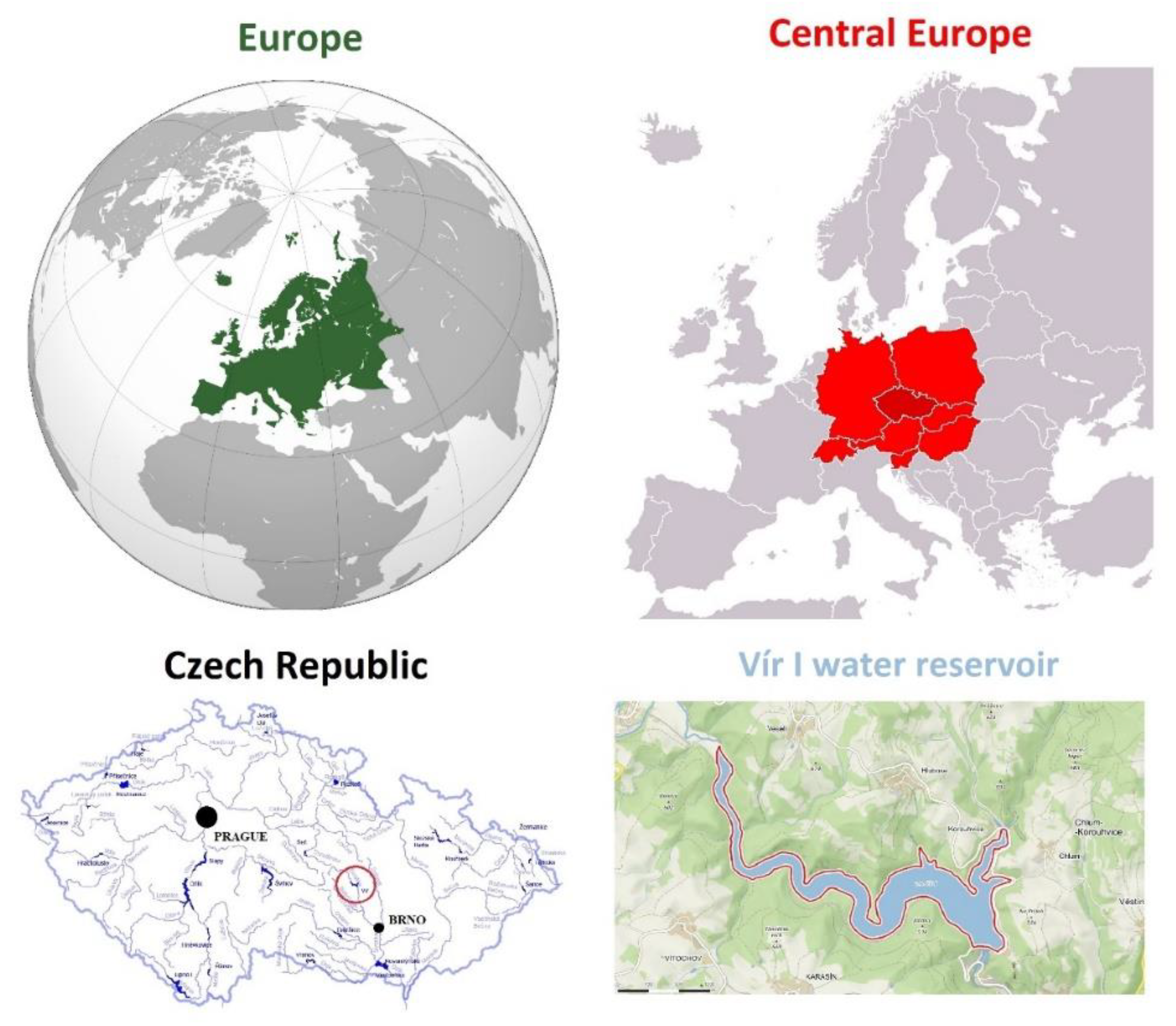
A case study was undertaken on the Vír I multi-purpose reservoir located on the Svratka River in the basin of the Morava River in the Czech Republic. The reservoir is located 150 km east of the capital city of Prague (see Figure 1) and supplies water to Brno, the second largest city. The concrete gravity dam falls under the administration of the Morava River Basin State Enterprise. The long-term inflow QA is 3.28 m3 s−1. The required water outflow from the reservoir OR is 2.5 m3 s−1. The storage volume VZ is 44.056 million m3 at an elevation of 464.45 m above sea level, the volume of inactive storage is 3.80 million m3, the retention volume VR is 8.337 million m3 and the total volume of the reservoir VTOT is 56.193 million m3. The reservoir has two bottom outlets with diameters of 1800 mm. At the maximum water level, the flow rate of the bottom outlets is maximally 2 × 40 m3 s−1. The emergency spillway of the reservoir is an uncontrolled crest structure at an elevation of 467.05 m above sea level, with a total length of 60.5 m (5 × 12.1 m) and a capacity of 180.5 m3 s−1 at the level of the uncontrollable retention volume. According to the Czech Technical Standard [12], the reservoir falls into category A, the highest priority, i.e., with a time reliability RT ≥ 99.5%. The main purposes of the reservoir are storage of drinking water and flood protection.
Hydrological data regarding the inflow of water into the reservoir used for the determination of the storage volume of the reservoir was in the form of historical monthly flows for the last 66 years and an updated flood discharge from 2008 was used to calculate the retention volume of the reservoir. Specifically, this was a flood discharge of Q1000 according to the classical regression without seasonality differentiation and with a time step of 360 min. Hydrological data were acquired from the Czech Hydrometeorological Institute.
The calculation of the storage volume of the reservoir aimed to take into account the losses of water from the reservoir, specifically evaporation from the water surface and seepage through the body of the dam. The amount of the evaporation was determined by the annual evaporation, i.e., 613 mm, and the seepage size through the dam body was 0.15 l s−1 per 1000 m2 [63].
4. Methodology
4.1. Problem Formulation
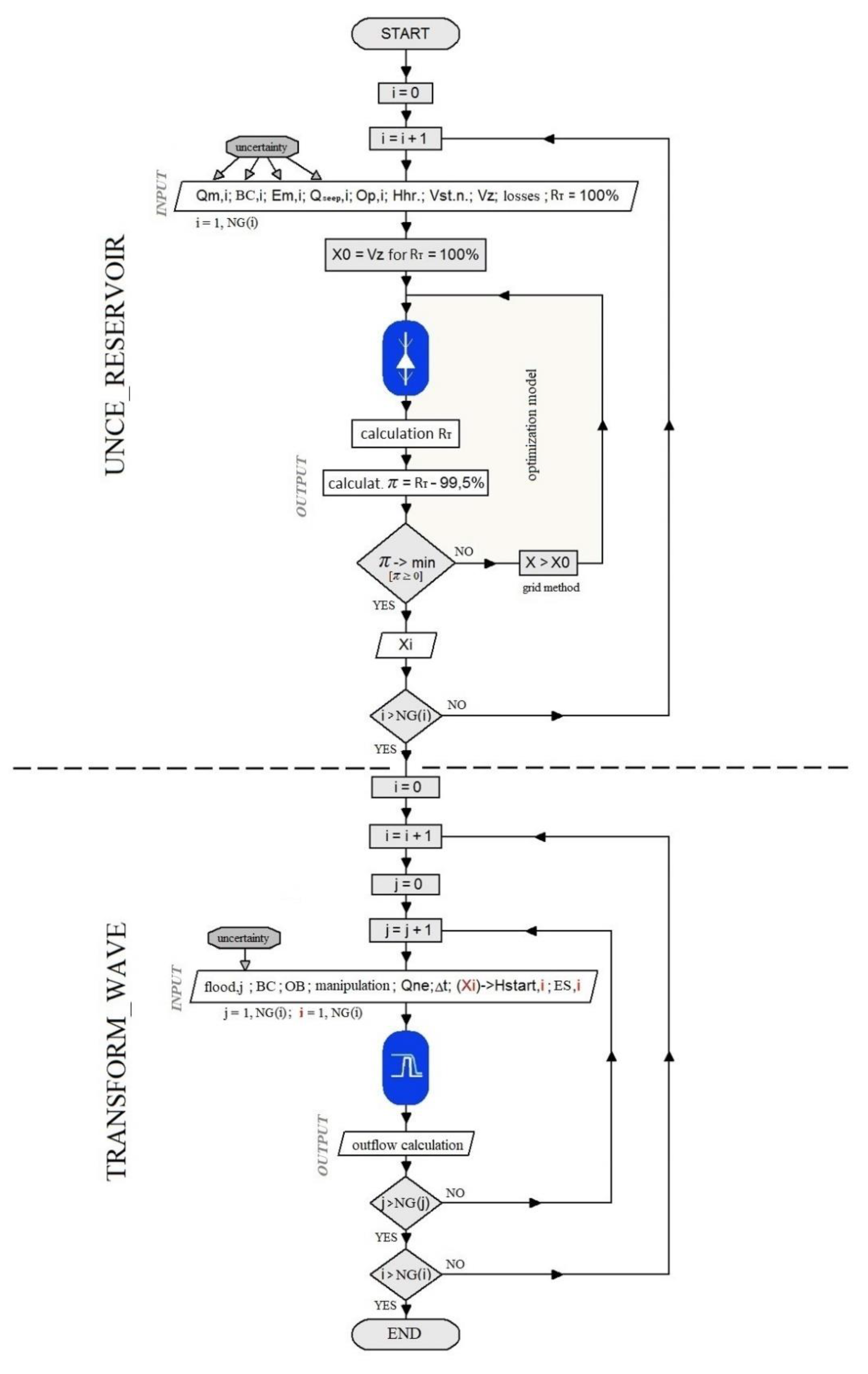
The operation of multi-purpose reservoirs is complicated due to the conflict between different objectives. In recent years, it has become desirable to maximize both storage volume and protective volume, as multi-purpose reservoirs may not fully respond to current and future climatic conditions. The solution is to find a suitable ratio between the size of the storage and the retention volume of water in the reservoir in conditions of uncertainty. In other words, we need to comprehensively determine the functional volumes of the reservoir. For this purpose, the models presented below apply input data uncertainties to their solution through the Monte Carlo method. The connection of both models for the determination of the functional volumes of the reservoir, including an example of the introduction of input uncertainties, is shown in the flow chart in Figure 2.
4.2. UNCE_RESERVOIR—Simulation-Optimization Model of the Reservoir for Determining the Storage Volume of the Reservoir
The developed simulation-optimization model determines the optimal storage volume of the reservoir VZ in conditions of uncertainty. To determine the optimal storage volume of the reservoir VZ = f(OR, RT), which is a function of the required outflow OR and predetermined temporal reliability RT < 100%, repeated calculations determining the temporal reliability RT = f(OR, VZ) at the predetermined required outflow OR and storage volume VZ were used.
The parameter sought was therefore the storage volume VZ. The criterion was temporal reliability according to the temporal reliability RT and the water management solution allowed water failures in the reservoir according to the categorization of the reservoir. The initial condition was a full reservoir at the beginning of the test period (a value of 0 on the left side of Equation (1) characterizes the full storage volume of the reservoir) and the boundary condition was a series of water inflows into the reservoir at the appropriate time steps. For each time step, a balance was made between the required outflow OR and the historical inflow of water into the reservoir Q. In addition, the limiting condition ∑(OR − Q) was tested, i.e., whether or not the reservoir was emptied at the end of each month (the VZ,MAX value on the right side of Equation (1) characterizes the empty storage volume of the reservoir). If it was emptied, a failure of the water outflow from the reservoir was judged to exist. This meant that in all months when the outflow of water Oi was less than the required outflow OR, the reservoir failed to supply enough water to the distribution system. The total sum of all failure months according to Equation (2) was recorded and the temporal reliability RT was calculated (see Equation (3)).
The basis of the simulation model of the subtask RT = f(OR, VZ) is the modified balance equation of the reservoir in the sum form converted into the following inequality (Equation (1)) [65]:
where Oi is the water outflow from the reservoir (m3 s−1) in a given month for i = 1, …, k; Qi is the inflow of water into the reservoir (m3 s−1) in a given month for i = 1, …, k and Δt is the time step of the calculation of one month.
The classification of the reservoir storage volume failure for the calculation of temporal reliability is expressed by Equation (2) [53]:
where Zt,i = 1 describes the state of the VZ reservoir in the fault-free (satisfactory) time step of the calculation and Zt,i = 0 describes the state of the VZ reservoir in the faulty (unsatisfactory) time step of the calculation.
The degree of temporal reliability of the improved outflow OR as a result of the outflow control is the probability that the actual outflow of water from the reservoir will not fall below the value of the improved outflow OR. In this case, the temporal reliability is applied according to the temporal reliability RT, which can be calculated from the values Zt,i according to Equation (2) [66]:
where is the sum of the records of the faulty and fault-free months and k is the number of all months of the input time series.
First, the value of the parameter (storage volume) is selected and a new variant of reservoir operation is repeatedly simulated according to Equation (1), and then the monitored criterion π (decrease in temporal reliability RT) is evaluated according to Equations (2) and (3). The solution is a variant in which the criterion coincides with the required value. In this variant, the selected parameter becomes the result of the solution. The task leads to an optimization in which the solved parameter is unknown and the criterion is the difference between the calculated and the required temporal reliability, which is minimized. The reservoir model uses a simple optimization method called the grid method, where parameters with a fixed step are selected at allowable intervals. The calculation also includes, among other things, water losses from the reservoir, specifically water losses by evaporation from the water surface and seepage of the dam body. The principle for introducing water losses from the reservoir into the solution is that the loss flows are counted using repeated simulation.
4.3. TRANSFORM_WAVE—Reservoir Simulation Model for Determining the Retention Volume of the Reservoir
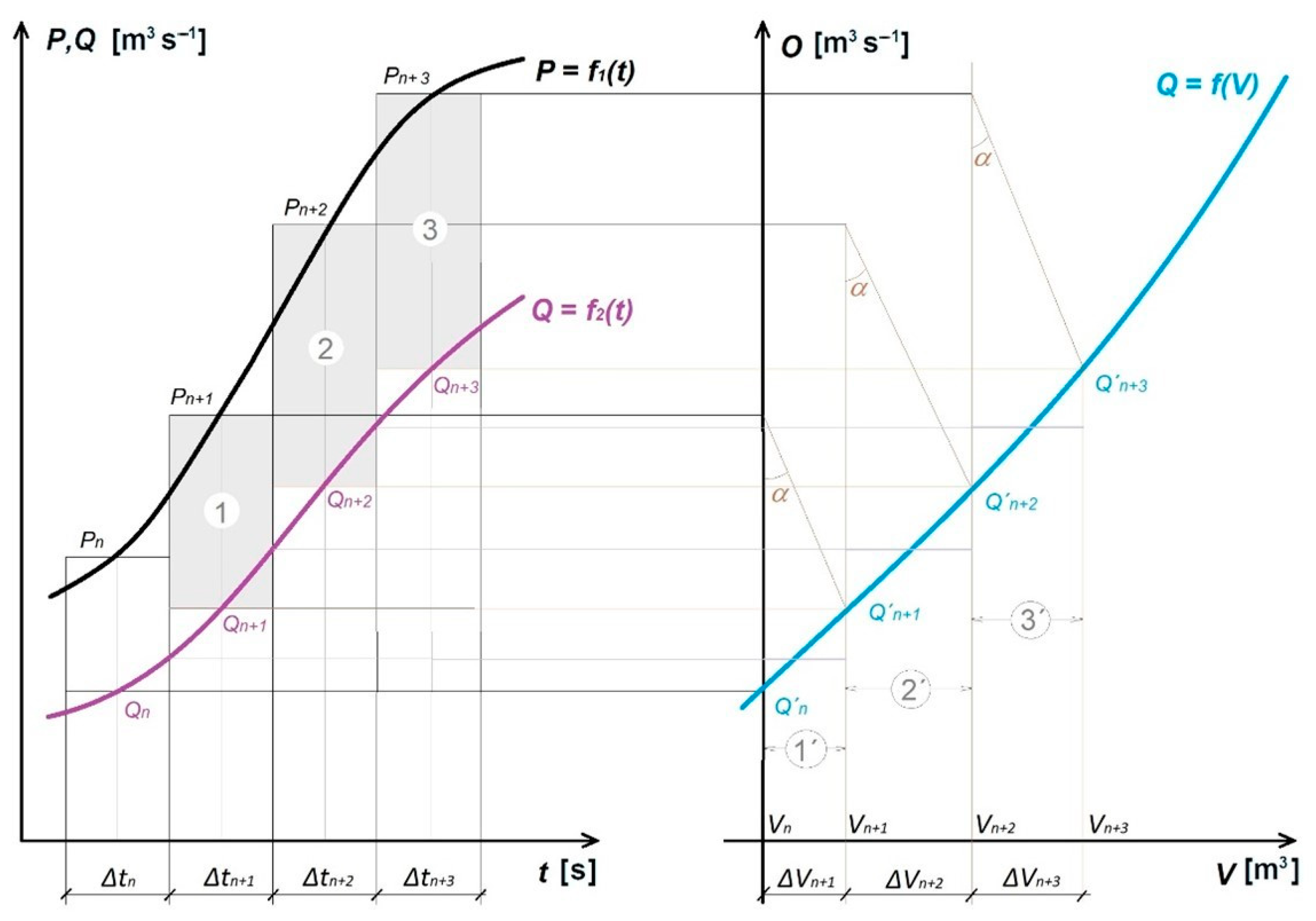
For the second hydrological extreme, flooding, a simulation model was developed for the transformation of uncertainty-affected flood discharges. In the model, the transformation of the flood discharge is performed by mathematical modification of the original Klemeš graphical method [43]. The Klemeš graphical method (see Figure 3) is based on the first order of the reservoir differential equation and expresses the relationship between the inflow and outflow of water from the reservoir as a function of time and the volume of water retained in the reservoir.
The following simplifications were introduced to construct the model: (i) Although the inflow and outflow values change continuously over a period of time during the process, they were considered to be constant in a given time interval. The inflow (marked as P and Q in Figure 3) and outflow in each interval are thus represented by a single instantaneous value; (ii) The Klemeš method was set to enter the calculation only when the emergency spillway is exceeded. If the water is below the level of the emergency spillway, then the calculation only balances the volume of water inflow and outflow to the previous reservoir volume.
The main data for the Klemeš method are the hydrograph of the flood, the parameters of the bottom outlets, the emergency spillway and the line of flooded volumes for the construction of the so-called transformation curve, which can be seen in the right part of Figure 3 and is marked as Q′. The transformation curve expresses the total outflow of water from the reservoir depending on its filling. It characterizes the potential outflow of water from the reservoir and is a function of the volume of the reservoir. To determine it, according to [67], the capacity of the bottom outlets OB should be calculated according to Equation (4) and the emergency spillway capacity QES according to Equation (5):
where μ is the outflow coefficient (-), S is the area of the outlet opening (bottom outlets) (m2), g is the gravity acceleration (m s−2), hw is the height of the water above the bottom outlets (m), m is the overflow coefficient (-), b is the width of the emergency spillway (m) and hes is the height of the water above the spillway (m).
Furthermore, it is necessary to use the Klemeš method to construct the reduction angle α for the transformation, which is based on the size of the flow and the time interval and characterizes the proportionality between the created area surrounded by inflow and outflow in a given time interval and the length of the horizontal line of the transformation curve of the given time interval. The graphical construction by the Klemeš method takes place gradually in individual time intervals, first on the ascending and then on the descending branch of the flood discharge, through the mentioned transformation curve and the reduction angle α.
4.4. Monte Carlo Method for Applying Input Uncertainties to the Reservoir Simulation Model
The following assumptions were introduced to create an algorithm that generates random series with a burden in the form of uncertainties. The general input value X resulting from the measurement was considered as a random (stochastic) quantity. This assumption makes it possible to generate new Xi values around the input value X resulting from the measurement completely randomly and independently of each other. The quantity Xi is therefore random and independent of the previous and following values. The randomly generated quantities Xi are the result of a number of mutually independent phenomena, which makes it possible to describe the input value with a corresponding normal probability distribution N(μ(X),σ(X)). The introduction of a normal probability distribution makes it possible to enter the vicinity of the resulting value of a random variable using the mean value μ(X) as the measured value and the standard deviations σ(X) as the standard uncertainty. Only the standard measurement uncertainty of type B uB,X was considered in the calculations. Finally, a simplification was introduced, whereby the standard uncertainty of measurement uB,X is deployed using the relative value of the coefficient of variation Cv(X) (see Equation (10)) and the resulting standard deviation σ(X) is then calculated according to Equation (9).
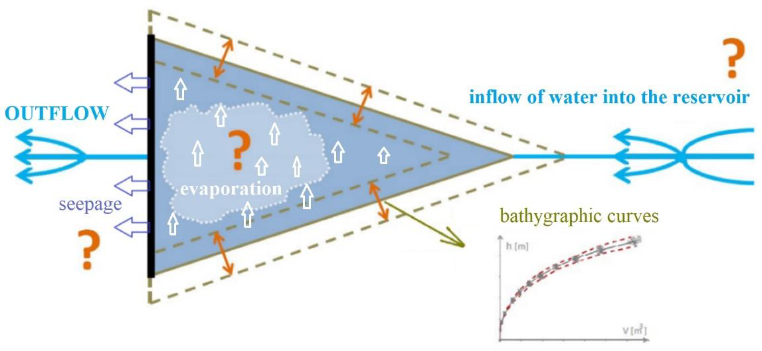
The essence of the random series generator is repeated use of the Monte Carlo method. Subsequently, for each mean value μt(X), distribution curves Ft(X) of the normal standardized probability distribution N(μ(X),σ(X)) are created for t = 1, 2, …, NE, where NE is the total number of elements (e.g., the total number of average monthly inflows or the total number of points from the flooded volume line). Using a pseudo-random number generator, generating random numbers from the interval ξ ∈ 〈0,1〉, random waveforms of a number of elements Xt are repeatedly generated, which are referred to as random positions of NXt,i values, in the interval of specified uncertainty for i = 1, 2, …, NG, where NG is the total number of repetitions (generations). The general principle for generating random positions of input parameters can be found in previous studies [52,53]. This described procedure for generating random elements can be applied to all quantities entering the water management solution for the storage and retention volume of the reservoir, except the bathygraphic curves of the reservoir. In this case, a compilation of two independent Monte Carlo generators was required. Each generator constructs a random point position (e.g., water level height) with a second random point position added to it (e.g., the volume of water in the reservoir). Together, the random positions of two points then create a random point coordinate (e.g., a random point coordinate of a flooded volume line). A series of random points then form random lines of flooded volumes burdened with uncertainties. A symbolic depiction of the introduction of considered quantities burdened with uncertainties is shown Figure 4.
4.5. Methods for Evaluation
The generated input uncertainties in the data for the calculation of the water management solution of the reservoir provide spectra of storage and retention volume sizes. For a suitable presentation of the achieved results, the calculations were statistically evaluated and quantiles and the overshoot probability curve were also used.
4.5.1. Mean Value
The mean value is the value of the first general moment, denoted as μ(X), and is expressed in the following form (Equation (6)):
The mean value belongs to the so-called position characteristics and its value is the x-coordinate of the center of gravity of the probability density. The method of moments involves an estimate of the mean value, as expressed by Equation (7):
where is the sample mean or mean value, xi are elements of random selection and n is the number of elements of random selection.
4.5.2. Variance and Standard Deviation
The standard deviation is expressed as the square root of the variance D(X). The variance rate of the random variable X regarding the diameter µX is given by the second central moment, or the variance D(X), which is expressed in the following form (Equation (8)):
The standard deviation is also based on the second central moment and is denoted by σ(x). Using the method of moments, the standard deviation is expressed by Equation (9):
4.5.3. Coefficient of Variation
Similar to the variance and standard deviation, the coefficient of variation is based on the second central moment. The coefficient of variation is denoted by Cv(x) and is expressed as the ratio of the standard deviation and the mean value (Equation (10)):
4.5.4. Coefficient of Variation
The overshoot probability function or overshoot probability curve determines the probability that a random variable will be greater than or equal to the value of A. The overshoot probability curve is a decreasing function and takes values from one to zero. It can be obtained by integration from the probability density on the right. The shape of the overshoot probability is given in Equation (11):
4.5.5. Quantile
The quantile indicates the measure of the position of the probability distribution of a random variable. In other words, quantiles describe the points at which the distribution function of a random variable passes through a given value. In the case of a continuous distribution having the distribution function Fx(x), the p-quantile xp is a value of a random variable X for which values less than xp occur only with probability p, i.e., for which the distribution function Fx(xp) is equal to the probability p (Equation (12)):
When presenting the results of quantiles in the overshoot probability function, 5, 10, 15, 20 and 25% quantiles correspond to the 95, 90, 85, 80 and 75% quantiles of the distribution function.
5. Results and Discussion
5.1. Storage Volume Modeling
It was first necessary to determine the inputs into the UNCE_RESERVOIR model for the updated length of the historical series of water inflows into the Vír reservoir up to 2018. In other words, it was necessary to determine the required water outflow from the OR reservoir for temporal reliability RT ≥ 99.5% and existing VZ. The calculation was performed without input uncertainties, including consideration of water losses from the reservoir. As a result, the OR had to be reduced to achieve a satisfactory RT = f(OR, VZ), as shown in Table 1.
In the next step, VZ was calculated deterministically and without input uncertainties, including the consideration of water losses from the reservoir for the calculated OR based on Table 1 and for RT ≥ 99.5%, i.e., the calculation of VZ = f(OR, RT = 99.5%). The resulting optimized VZ should be close to the real reservoir volume. Based on the comparison of the optimized VZ with the real VZ, the OR was slightly changed. These values are given in Table 2 along with the OR value for the further calculations that follow.
After determining the exact value of OR needed to meet the significance of the reservoir with regard to the updated line of water inflow into the reservoir and the resulting VZ approaching the real VZ, the optimized storage volumes VZ of the reservoir for the whole range of water inflow into the reservoir and with input uncertainties were calculated and evaluated. Input uncertainties from the measurements were applied: (i) constantly for all inputs with sizes uB = ±1, ±2, ±3, ±5 and ±7% and (ii) differently for entered values according to the probable size of uncertainty for each input; specifically, ±3% for the inflow of water into the reservoir, ±5% for bathygraphic curves, ±4% for evaporation and ±3% for seepage through the reservoir body. The number of repetitions (generations) NG was always set to 300 repetitions.
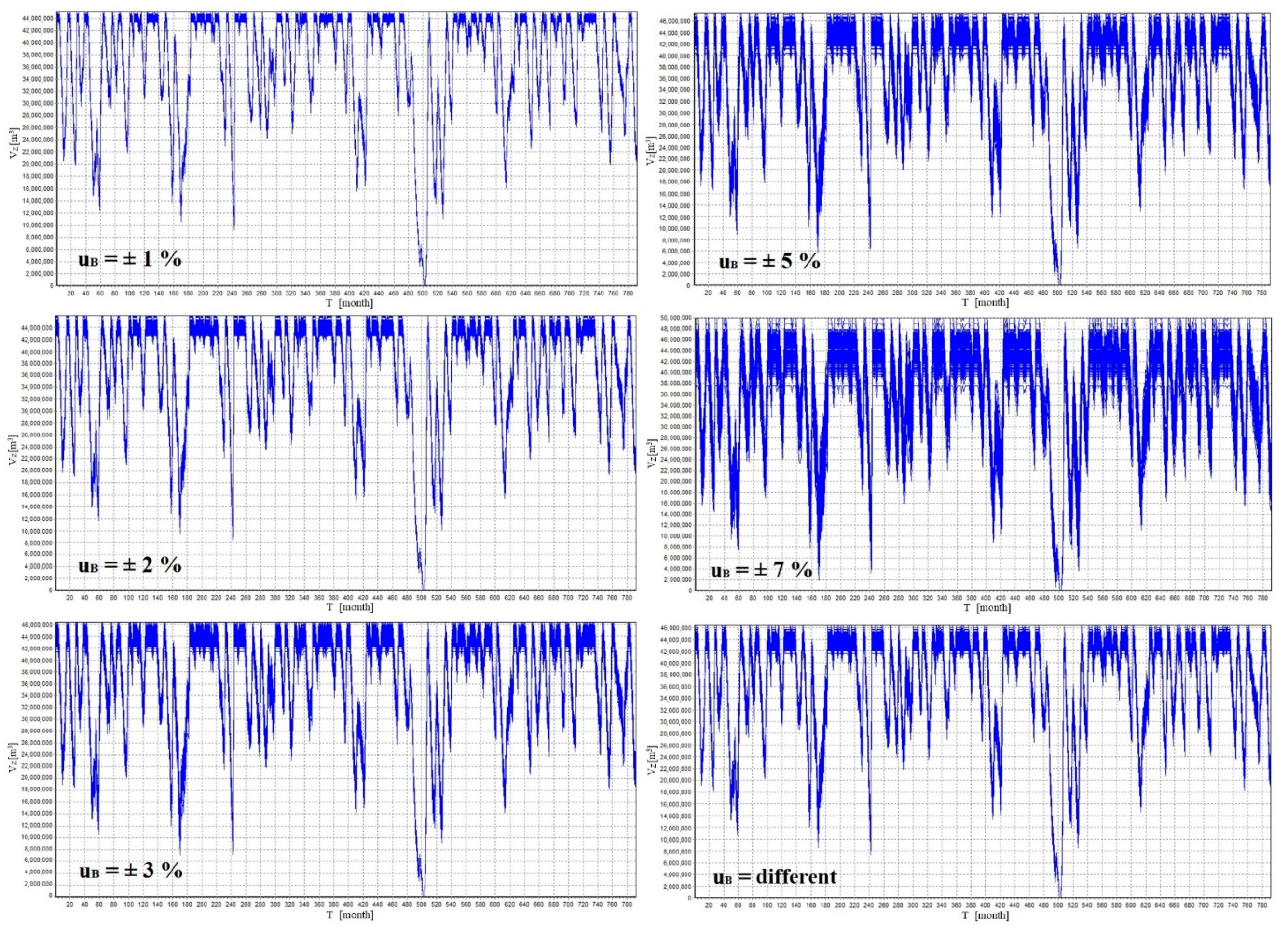
Figure 5 shows the calculated filling and emptying curves. These curves are shown for all considered input uncertainties and Table 3 shows the calculated mean values of the optimized stock volumes, including standard deviations. Furthermore, these results were evaluated by adding the upper and lower limits through a coefficient of expansion k = 2, which corresponds to a probability density coverage of approximately 95%. The last line also shows the 95% quantile of the optimized storage volume of the tested reservoir.
The reservoir filling and emptying courses shown in Figure 5 effectively demonstrate the increase in the variance of possible solutions with increasing input uncertainties, which is also evident in Table 3. Different input uncertainty settings according to the probable uncertainty affected the reservoir filling and emptying courses as an approximate uniform input uncertainty setting of uB = ±3%.
For the probable sizes of the input data uncertainty (different), the resulting optimized storage volume of the reservoir for 95% probability coverage was 44.149 million m3 ± 1.622 million m3, i.e., the result lay in the interval {42.527 million m3; 45.771 million m3}. To be on the safe side, it is desirable to work with the resulting upper interval, i.e., a higher storage volume, in a stochastic solution. Expressed by the 95% quantile, the resulting optimized volume was 45.628 million m3; compared to the upper quantile, this value of VZ is 0.31% lower. The relatively safe and therefore recommended final value of the storage volume from this analysis was 45.770 million m3. Based on the updated input series of water inflows into the reservoir and the introduction of input uncertainties, including consideration of water losses from the reservoir, it is therefore recommended that the existing storage volume of the Vír I reservoir be increased by up to 3.9%, specifically by 1.71 million m3.
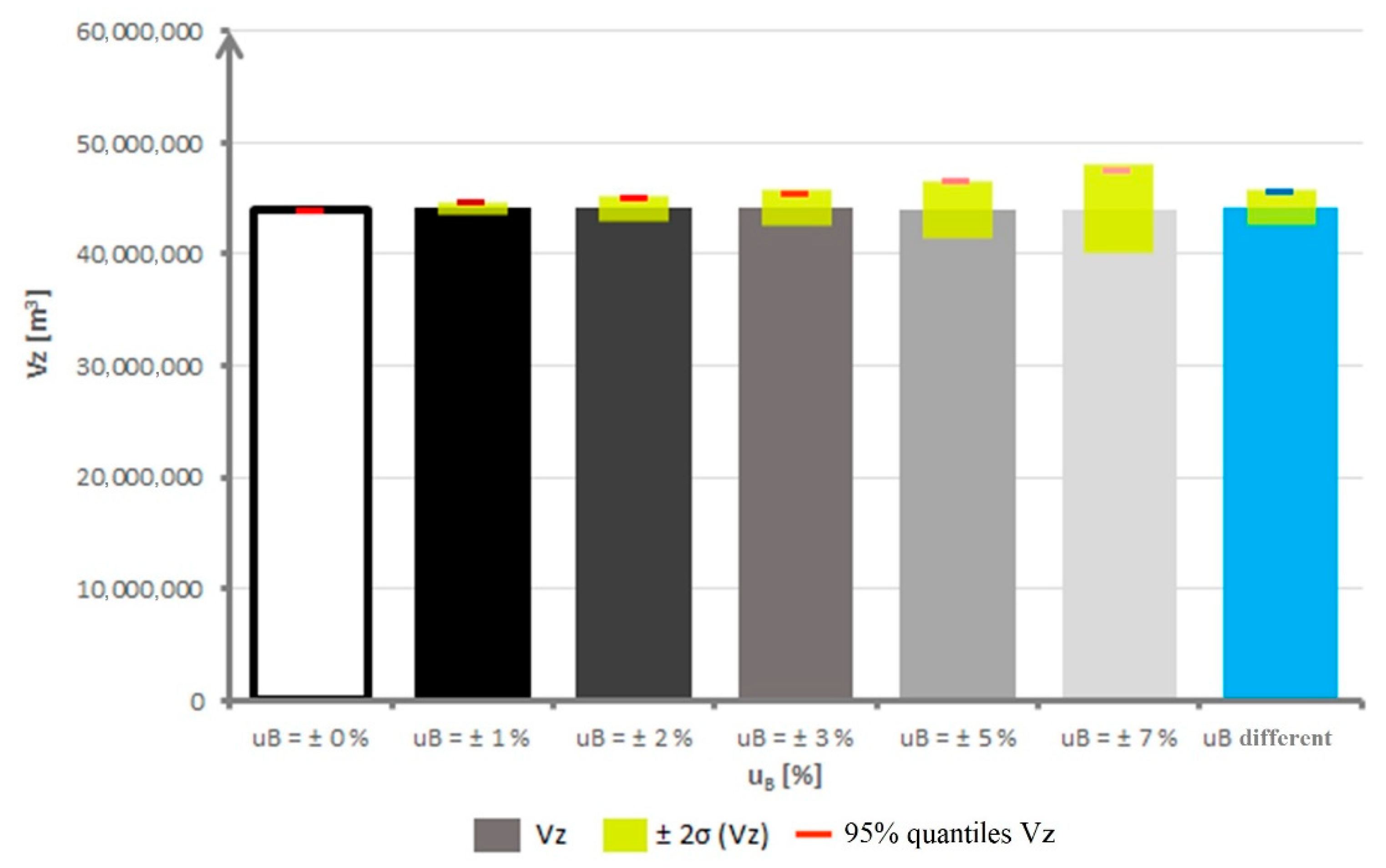
The results from Table 3 are also presented in the form of a bar chart in Figure 6, where the resulting optimized stock volumes for all tested input uncertainties are plotted. The lower and upper limits for ±2 standard deviations of the storage volumes are marked in yellow and the solution using the 95% quantiles in red. The final bar in blue depicts the results for VZ with the probable different input uncertainties.
Furthermore, increases in the values of the variances of the resulting optimized storage volumes ±2σ(VZ) compared to the existing VZ depending on the input uncertainties uB were expressed as percentages. The results are shown in Table 4.
Table 4 shows that, for the tested reservoir Vír (line two), the results in the form of ±2σ(VZ) demonstrate a steady increase depending on uB. Testing on another reservoir, Vranov (line three), showed that there are not always such steady increases in results but that these depend on the growing uncertainties of the input data. Thus, different reservoirs can react completely differently to input uncertainties.
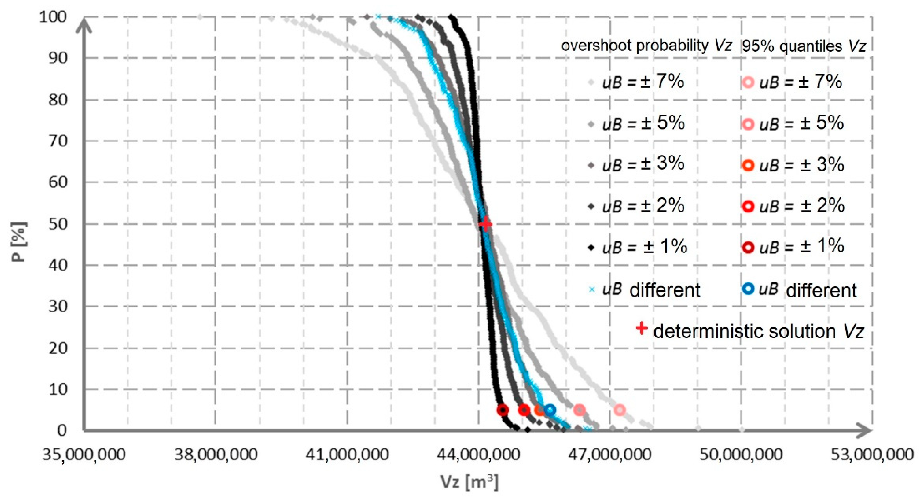
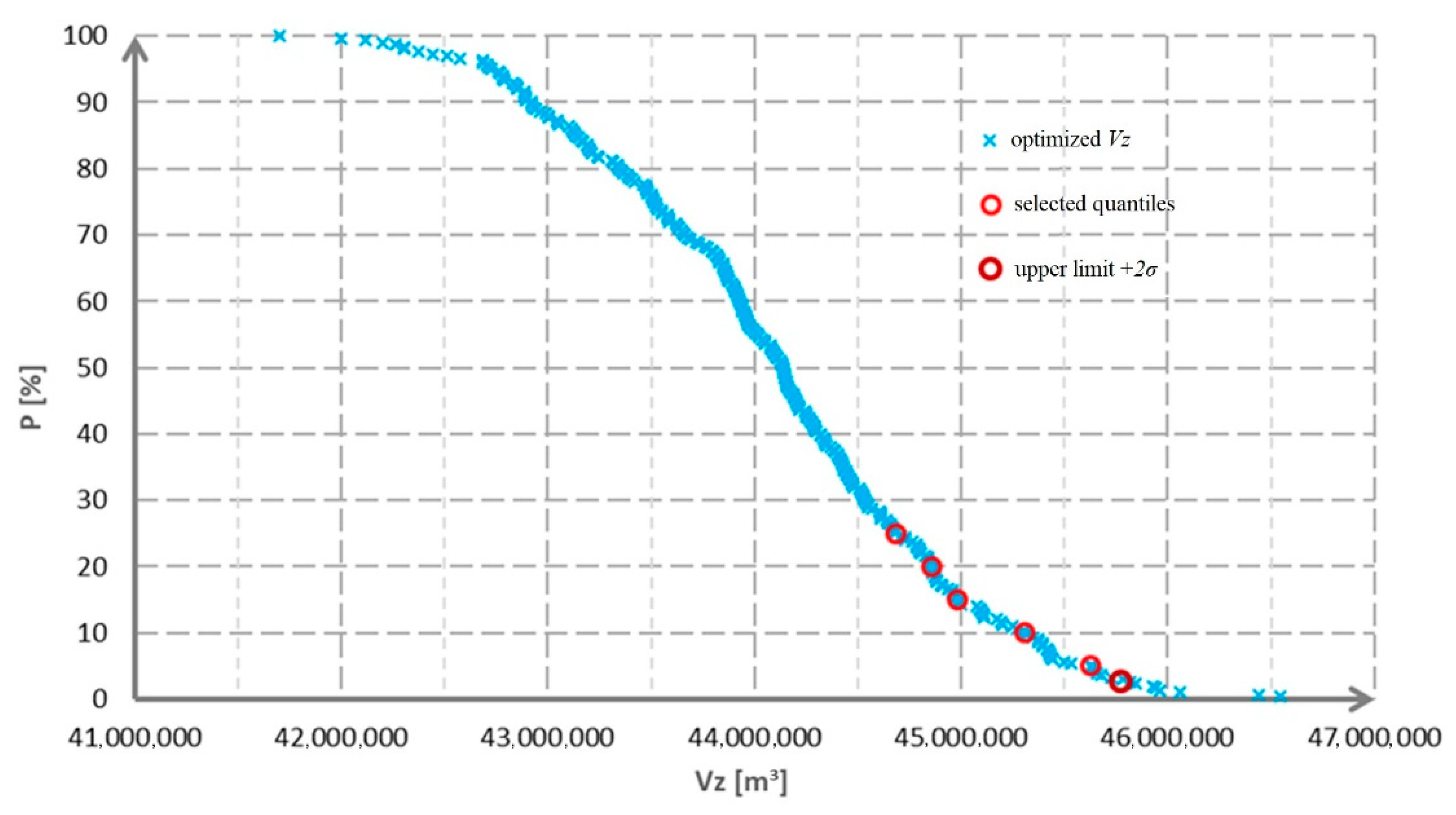
The results for the sets of optimal reservoir storage volumes obtained from the reservoir filling and emptying process depicted in Figure 5 are shown in Figure 7 in the form of an empirical overshoot probability curve. Each empirical curve consists of 300 final values for optimal storage volumes VZ, which were sorted from minimum to maximum. Each overshoot probability curve corresponds to one type of input uncertainty setting. Furthermore, the 95% quantile (i.e., 5%) used for evaluation is marked on each curve.
In Figure 7 we can see that, for the probability P = 50%, the optimized values of VZ for all courses take on values just above 44 million m3, which is similar to the deterministic solution VZ = 44.056 million m3. This confirms the correctness of the random number generator. The courses of the individual curves are relatively symmetrical. The resulting mean values of the optimized storage volumes μ(VZ) in Table 3 increase in comparison with the current value of the storage volumes by percentage values from 0.10% (for uB = ±5%) to + 0.22% (for uB = ±3%). The average of deviations for all input uncertainties was about + 0.09%. The obtained results for the stochastic optimized storage volumes reach only slightly higher values than in the deterministic solution. These factors again confirm the correctness of the random number generator and the appropriateness of using the Monte Carlo method.
5.2. Retention Volume Modeling
Further calculations were performed to determine how increasing the storage volume of the reservoir can affect the transformation of the flood discharge and the change in the retention volume of the reservoir. For this calculation, several variants of the design of the storage volume of the reservoir were considered. The developed simulation optimization model UNCE_RESERVOIR (described in Section 4.2) makes it possible to store all calculated optimal storage volumes according to the number of set repetitions and then to calculate the retention volume of the reservoir for any number of repetitions for each of these volumes using the second simulation model, TRANSFORM_WAVE (described in Section 4.3). To simplify and shorten the calculation time, only a few optimal storage volumes were selected to obtain a single complex solution of functional volumes out of 300 possible solutions with input uncertainties entered differently (according to the probable size of uncertainty at each input), i.e., the blue course of the probability curve in Figure 7. Specifically, the optimal storage volumes resulting from 75, 80, 85, 90 and 95% quantiles (i.e., 25, 20, 15, 10 and 5% in the overshoot probability function) and the upper limit of the resulting expanded uncertainty +2σ were selected from this calculation setting (see Figure 8).
For the selected optimal VZ values of the reservoir, Table 5 shows the specific VZ values of the optimal storage volumes in column three and the corresponding water heights in the reservoir hVz in column two. It is clear that, with the increasing quantile (downwards in Table 5), the optimal value of VZ increases and therefore the height of water in the reservoir hVz also increases. Since the emergency spillway of the reservoir is always considered at the same height hVRC (column four) in accordance with the chosen location, the increase of controllable retention VRC (column five) and hVRC is at the expense of the uncontrollable retention volume hVRU (column six) and VRU (column seven).
To calculate the retention volume, a flood discharge Q1000 with an input standard uncertainty uB = ±10% was selected, which was chosen as the minimum following [68], in which the reliability classes of hydrological data are given, including the probable variance of errors. The calculation was performed in the variant without pre-drainage of water from the reservoir. The number of uncertainties generated for the flood discharge was chosen to be 300 repetitions. The starting water level in the reservoir at the beginning of the flood discharge transformation solution was always the full storage volume VZ, i.e., the newly calculated height hVz. Based on the above information on bottom outlets and the emergency spillway along with Equations (4) and (5), the outlet coefficient of the bottom outlets or the outflow coefficient μ and the overflow coefficient m were determined. Specifically, for the tested reservoir, the outflow coefficient μ = 0.435 (-) and overflow coefficient m = 0.407 (-). In the variant without pre-drainage, the level is kept at the level of the full storage volume and, as soon as this level is exceeded, the bottom outlets are opened to a harmless flow QNE. When the emergency spillway is exceeded, the bottom outlets are smoothly closed and, after the flooding, they are smoothly opened to a water height of 0.5 m above the emergency spillway. The level after the flood is again kept at the level of the full storage volume.
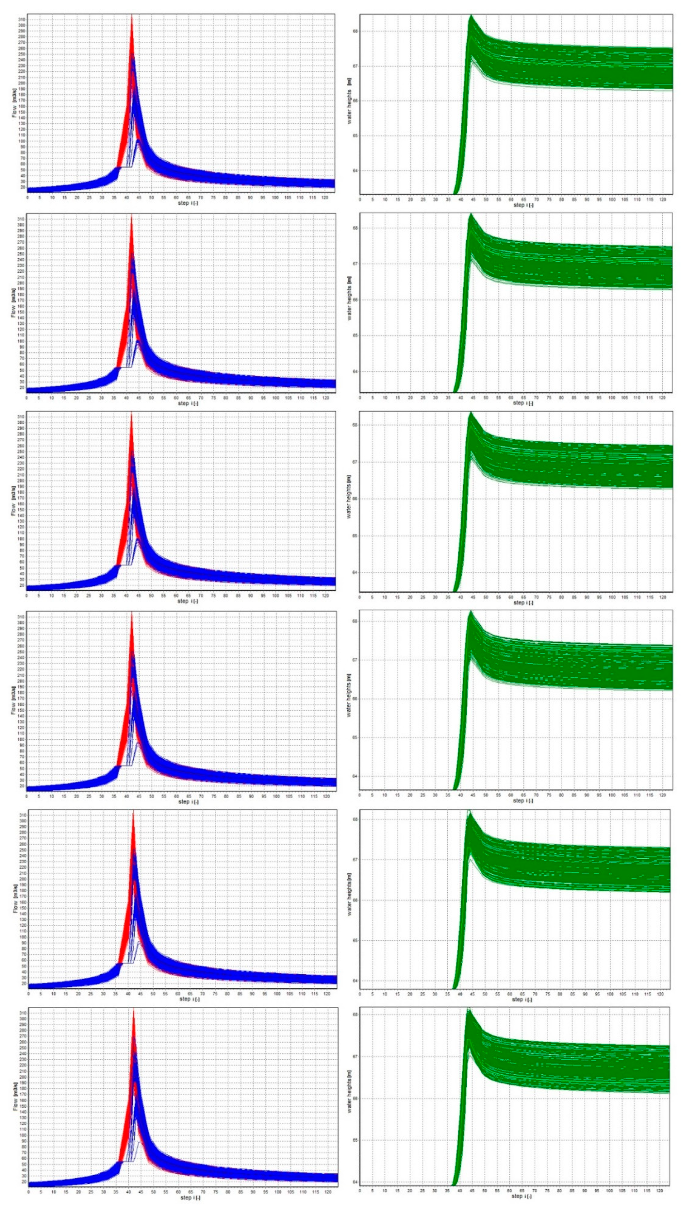
Figure 9 shows the results of individual transformations for selected optimal VZ values. The generated courses of these flood discharges are shown here in red, the results of the transformed waves in blue and the courses of the water heights in the reservoir during the transformations in green.
In Figure 9, the transformations of the generated flood discharges have similar courses and there are also similar courses in the heights reached, with the only difference being that the starting level is from the selected optimal VZ. The input uncertainty has a clear effect on flood discharges but also on the results of transformed floods and water heights in the reservoir.
5.3. Summary of Results
It is worth noting the creation of several bundles of transformed flood discharges (blue lines), which are probably caused by the size of the time step. When the emergency spillway is exceeded in another time step, the difference is at least one time step, i.e., 6 h, which is a consequence of the formation of bundles and jumps in the peaks of the transformed floods. If the time step were finer, these bundles would not be formed and the courses of the transformed floods, including peaks, would be spread more smoothly.
Comparing the results for the starting height of 63 m from the existing storage volume, a slight decrease in the peak of the water heights in the reservoir is evident. This decrease is also confirmed in Table 5, specifically in column six, i.e., the height hVRU, the height of the uncontrollable retention volume or the achieved peak of the height of the water in the reservoir during the transformations of flood discharges. These values include the expanded uncertainty of ±2σ. In Table 5, column seven then shows the results of the uncontrollable retention volume VRU, including the upper limit of the expanded uncertainty +2σ. Furthermore, column eight shows the total volume of the retention volume VR, including the upper limit of the expanded uncertainty +2σ (bold), and the total volume of the reservoir VTOTAL is shown in column nine. Finally, the last columns, 10 and 11, show the values of Q1000 flood peaks, including the expanded uncertainty ±2σ, and the height between the uncontrollable retention volume (maximum water level in the reservoir) and the control maximum level CML (dam height), including the upper limit of the expanded uncertainty +2σ (bold).
In Table 5, we can see the results from the transformations of the generated flood discharges for selected optimal values VZ. Specifically, the first row shows the values for the current state of the reservoir according to [63] and the second row contains the results of the transformation of the flood discharge Q1000 for the current state of VZ. The following rows show the results for selected quantiles of optimal VZ values.
The results in Table 5 show that, with a higher storage volume at a constant emergency spillway height (hVRC level), the following decrease: (i) the controllable retention volume VRC, (ii) the height of the uncontrollable retention volume hVRU, (iii) the uncontrollable retention volume of the reservoir VRN, (iv) the retention volume of the reservoir VR and (v) the total reservoir volume VTOTAL. The decrease in hVRU has the effect of increasing the difference in size between the hVRU and CML (column 11), which is desirable for the solution. On the other hand, the peak flow QPEAK increases. It should be noted that, although the values of volumes and heights decrease (columns five to nine), they are significantly higher (lower for column 11) than the actual values of the existing tested reservoir.
This is because a given higher value VZ (starting level) corresponds to a larger volume from the line of flooded volumes and, therefore, more water is captured in the initial flood step and subsequent steps than at the starting height of 63 m. As a result, the resulting retention volume and total reservoir volume decrease with increasing height VZ. In contrast, the difference between the hVRU and CML increases, which is a key parameter when designing or changing the functional volumes of a reservoir. This suggests a design for the safest solution in terms of optimal VZ, i.e., either the 95% quantile of VZ or the upper limit of VZ (+2σ). In these designs, the increases in the retention volume VR by 1.37 million m3 and 1.09 million m3 would correspond to increases of 16.5% and 13.1% compared to the actual VR. However, we must not forget that with this choice the peak flow of the transformed flood discharge increases. For example, for the transformation from the current state, the peak flow of the upper limit of the expanded uncertainty (+2σ) is 234.65 m3 s−1 and, for the transformation from the 95% quantile of VZ, the peak flow is 248.82 m3 s−1, which is another key parameter in the design of functional volumes of a reservoir.
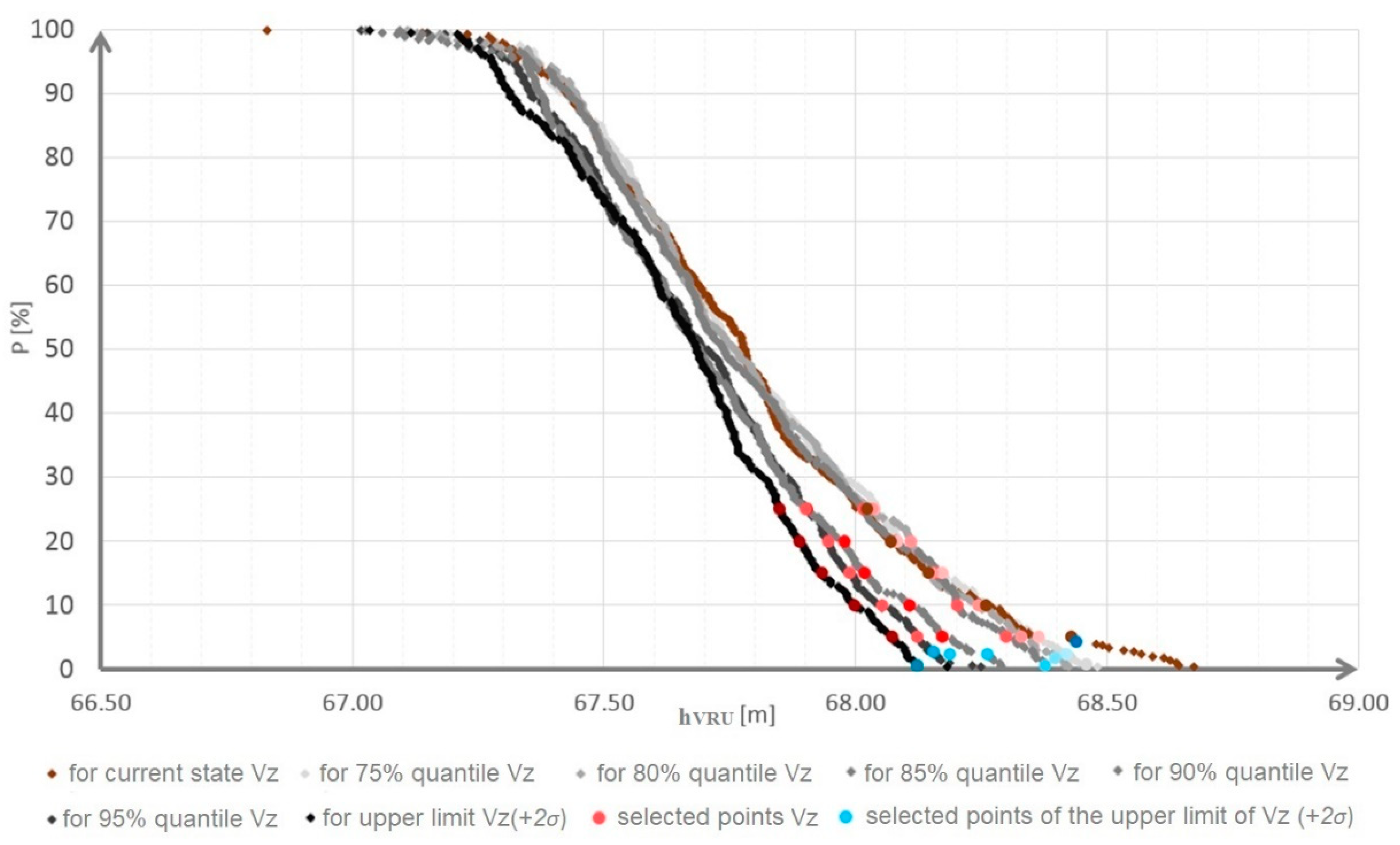
Finally, the calculated retention volumes of water in the reservoir for selected optimal VZ values were also evaluated using quantiles, as was the case with the storage volume of the reservoir. Figure 10 shows the results of water height peaks in the reservoir during transformations of generated flood discharges burdened with input uncertainties uB = ±10% in the form of the probabilities of exceeding these peaks for selected optimal storage volumes (black and white shades) and for the current reservoir storage volume (brown shade).
In Figure 10 we can see again that at a higher starting height (higher percentage of VZ quantiles) lower peaks of the water level in the reservoir are achieved, i.e., the hVRU level or the maximum water level in the reservoir does not rise so high. At the same time, selected quantiles and the upper limit +2σ are marked on the plotted curves, similarly to the selection of optimized VZ. The complete results for the water height peaks in the reservoir with possible functional volumes are summarized in detail in Table 6, which is designed in the same form as Table 5. This table shows the results of flood discharge transformations for selected quantiles and the upper limit +2σ. Peak flow QPEAK is expressed for the given variants in the form +2σ.
Table 6 shows that the most suitable solution is at the bottom of the table. It consists in a significant increase in VZ at the expense of the size of the flood peak because, with such a solution, higher water height peaks in the reservoir during the transformation are achieved but, at the same time, there is a greater height between the hVRU and CML. In the case of large floods, which the Q1000 undoubtedly is, the safety of the dam itself must be considered, i.e., elimination of the overflow of the CML.
6. Conclusions and Recommendations
This article applied the uncertainties resulting from the measurements that enter into water management solutions to a case study of the Vír reservoir, Czech Republic. For this reservoir, the following were developed and tested: (i) a simulation-optimization model that determines the optimal storage volume of the reservoir and (ii) a simulation model for the transformation of uncertain flood discharges that determines the retention volume of the reservoir. The obtained results lead to the following key conclusions:
- Input uncertainty significantly affects the results of VZ and VR calculations.
- To be on the safe side, it is appropriate to increase the values of either VZ or VR in accordance with the calculated uncertainties. Specifically, the input uncertainties discussed here highlighted the need to increase the existing VZ of the tested reservoir by up to 1.71 million m3 (3.9%) and the existing VR by up to 1.37 million m3 (16.5%).
- For a comprehensive determination of functional volumes, calculations of the transformation of the updated flood discharge burdened with uncertainty for selected optimal values of VZ were performed. These led to the determination of how an increase in VZ can affect the transformation of the flood discharge and the change in the VR of the reservoir.
- Based on the above, Table 6 was created with solution options for VZ and VR under conditions of uncertainty, including possible flood peaks and water height peaks in the reservoir.
- The developed simulation-optimization (i) and simulation (ii) models of the reservoir, the methods used and the introduction of uncertainties on the input data proved their functionality in solving the functional volumes of the water in the reservoir.
- Uniqueness can be observed in the connection between the solutions of the functional volumes of the reservoir for input data under conditions of uncertainty.
- The source codes of both models are written in such a way as to maintain generality and thus can be quickly used to test other existing or planned reservoirs anywhere in the world, if suitable data are available.
The introduction of uncertainties into the input data and their subsequent analysis proved the influence of extreme values on the final solution. It can be assumed, that even for other reservoirs with different input uncertainties, such uncertainties will have an impact on the existing functional volumes of these reservoirs. This only confirms the importance of this issue and highlights the need for detailed analyses of waterworks.
The models were applied to an updated historical series dating up to the present, i.e., in a period that can be considered a period with ongoing climate change. In addition, the assumption of uncertainty in the measurement of input data was incorporated into the solution.
From the point of view of measurement uncertainty and climate change uncertainty, the achieved results are relevant to the first stage of water management analyses, which involves capturing possible changes in the development of hydroclimatic extremes. In other words, the volumes of reservoirs are assessed with regard to their current state but with the assumption that they must incorporate the already ongoing process of climate change.
In the second stage of the solution, inputs can be inserted into the models to capture the future uncertainty of climate change thanks to the general notation of the source codes of the models. Instead of historical series of water inflows into the reservoir, simulations of non-stationary hydrological flow series, hydrological time series with negative trends of flow development or directly hydrological simulations describing climate change based on climate model scenarios can be used.
Likewise, flood discharges can be entered in the form of real extreme floods, artificial flood hydrographs or predicted floods affected by climate change.
Although the present analysis was performed for only one reservoir and the results cannot be generalized at present, the created software tool as a whole allows the analysis of existing reservoirs, or the dimensioning of new reservoirs, during the ongoing process of climate change under conditions of extreme fluctuation and for non-stationary hydrological data around the world.
Author Contributions
Conceptualization, S.P. and D.M.; methodology, S.P. and D.M.; software, S.P. and D.M.; validation, S.P.; formal analysis, S.P.; investigation, S.P.; resources, S.P.; data curation, S.P. and D.M.; writing—original draft preparation, S.P.; writing—review and editing, S.P. and D.M.; visualization, S.P.; supervision, D.M.; project administration, S.P.; funding acquisition, S.P. and D.M. All authors have read and agreed to the published version of the manuscript.
Funding
This research was funded by “Effective management of water resources in South Moravia”, research project number [FAST-S-20-6346].
Institutional Review Board Statement
Not applicable.
Informed Consent Statement
Not applicable.
Data Availability Statement
Not applicable.
Conflicts of Interest
The authors declare no conflict of interest.
References
- WMO. Statement on the State of the Global Climate in 2019; World Meteorological Organization: Geneva, Switzerland, 2020; ISBN 978-92-62-11248-5. [Google Scholar]
- IPCC. Global Warming of 1.5 C. An IPCC Special Report on the Impacts of Global Warming of 1.5 C above Pre-Industrial Levels and Related Global Greenhouse Gas Emission Pathways, in the Context of Strengthening the Global Response to the Threat of Climate Change, Sustainable Development, and Efforts to Eradicate Poverty; MassonDelmotte, V., Zhai, P., Portner, H.O., Roberts, D., Skea, J., Shukla, P.R., Pirani, A., Moufouma-Okia, W., Péan, C., Pidcock, R., et al., Eds.; IPCC: Geneva, Switzerland, 2018; Available online: http://ipcc.ch/report/sr15/ (accessed on 20 February 2021).
- Trnka, M.; Vizina, A.; Hanel, M.; Balek, J.; Hlavinka, P.; Semerádová, D.; Chuchma, F.; Dumbrovský, M.; Daňhelka, J.; Dubrovský, M.; et al. Pozorované Změny a Výhled pro Vodní Bilanci a Potřebu Vody v Zemědělské Krajině České Republiky. Vodohospodářská Konference Vodní Nádrže 2017; Povodí Moravy: Brno, Czech Republic, 2017; ISBN 978-80-905368-5-2. [Google Scholar]
- Zahradníček, P.; Trnka, M.; Brázdil, R.; Možný, M.; Štěpánek, P.; Hlavinka, P.; Žalud, Z.; Malý, A.; Semerádová, D.; Dobrovolný, P.; et al. The extreme drought episode of August 2011–May 2012 in the Czech Republic. Int. J. Clim. 2015, 35, 3335–3352. [Google Scholar] [CrossRef]
- Duchan, D.; Dráb, A.; Říha, J. Flood Protection in the Czech Republic. In Management of Water Quality and Quantity; Springer Nature: Cham, Switzerland, 2019; pp. 333–363. ISBN 978-3-030-18358-5. [Google Scholar]
- Stahl, K.; Hisdal, H.; Hannaford, J.; Tallaksen, L.M.; van Lanen, H.A.J.; Sauquet, E.; Demuth, S.; Fendekova, M.; Jódar, J. Streamflow trends in Europe: Evidence from a dataset of near-natural catchments. Hydrol. Earth. Syst. Sci. 2010, 14, 2367–2382. [Google Scholar] [CrossRef] [Green Version]
- Hanel, M.; Kašpárek, L.; Mrkvičková, M.; Horáček, S.; Vizina, A.; Novický, O.; Fridrichová, R. Odhad Dopadů Klimatické Změny na Hydrologickou Bilanci v ČR a Možná Adaptační Opatření; Výzkumný Ústav Vodohospodářský T. G. Masaryka, v.v.i: Praha, Czech Republic, 2011; ISBN 978-80-87402-22-1. [Google Scholar]
- IPCC. Summary for Policymakers, Climate Change 2014, Synthesis Report. Contribution of Working Groups I, II and III to the Fifth Assessment Report of the Intergovernmental Panel on Climate Change; Core Writing Team, Pachauri, R.K., Meyer, L.A., Eds.; IPCC: Geneva, Switzerland, 2014. [Google Scholar]
- Der Kiureghian, A.; Ditlevsen, O. Aleatory or epistemic? Does it matter? Struct. Saf. 2009, 31, 105–112. [Google Scholar] [CrossRef]
- Dantan, J.; Gayton, N.; Qureshi, A.; Lemaire, M.; Etienne, A. Tolerance Analysis Approach based on the Classification of Uncertainty (Aleatory/Epistemic). Procedia CIRP 2013, 10, 287–293. [Google Scholar] [CrossRef] [Green Version]
- Czech Government Document: Strategie Přizpůsobení se Změně Klimatu v Podmínkách ČR. Ministerstvo Životního Prostředí. 2015. Available online: http://www.mzp.cz/C1257458002F0DC7/cz/zmena_klimatu_adaptacni_strategie/$FILE/OEOK-Adaptacni_strategie-20151029.pdf (accessed on 1 October 2020).
- Czech Technical Standard ČSN 75,2405 Reservoir Storage Capacity Analysis. Available online: https://csnonline.agentura-cas.cz/Detailnormy.aspx?k=501441 (accessed on 3 October 2020).
- Knight, F.H. Risk, Uncertainty, and Profit; Boston, Hart, Schaffner & Marx; Houghton Mifflin Company: Boston, MA, USA, 1921. [Google Scholar]
- WECC doc. 19–1990:”Guidelines for Expression of the Uncertainty in Calibrations”. 1990. Available online: http://www.qcalibration.com/image/uncertainty.pdf (accessed on 1 October 2020).
- International Organization for Standardization. Guide to the Expression of Uncertainty in Measurement; International Organization for Standardization: Geneva, Switzerland, 1993. [Google Scholar]
- Document: Expression of the Uncertainty in Measurement in Calibration. EAL Task Force, EA 4/02. 1999. Available online: https://www.isobudgets.com/pdf/uncertainty-guides/european-co-operation-for-accreditation-ea-4-02-m-1999-expression-of-the-uncertainty-of-measurement-in-calibration.pdf (accessed on 3 October 2020).
- Document: ISO GUM Suppl. 1 (DGUIDE 99998). Guide to the Expression of Uncertainty in Measurement (GUM)—Supplement 1: Numerical Methods for the Propagation of Distributions; International Organization for Standardization: Geneva, Switzerland, 2004; Available online: http://geste.mecanica.ufrgs.br/medterm/ISO_GUM_sup1.pdf (accessed on 3 October 2020).
- Beven, K.J.; Binley, A.M. The future of distributed models: Model calibration and uncertainty prediction. Hydrol. Processes 1992, 6, 279–298. [Google Scholar] [CrossRef]
- Beven, K. Towards integrated environmental models of everywhere: Uncertainty, data and modelling as a learning process. Hydrol. Earth Syst. Sci. 2007, 11, 460–467. [Google Scholar] [CrossRef]
- Baldassarre, G.D.; Montanari, A. Uncertainty in river discharge observations: A quantitative analysis. Hydrol. Earth Syst. Sci. 2009, 13, 913. [Google Scholar] [CrossRef] [Green Version]
- Shrestha, R.R.; Simonovic, S.P. Fuzzy set theory based methodology for the analysis of measurement uncertainty in river discharge and stage. Can. J. Civ. Eng. 2010, 37, 429–439. [Google Scholar] [CrossRef]
- Tomkins, K.M. Uncertainty in streamflow rating curves: Methods, controls and consequences. Hydrol. Process. 2012, 28, 464–481. [Google Scholar] [CrossRef]
- Westerberg, I.K.; McMillan, H.K. Uncertainty in hydrological signatures. Hydrol. Earth Syst. Sci. 2015, 19, 3951–3968. [Google Scholar] [CrossRef] [Green Version]
- Westerberg, I.K.; McMillan, H.K. Uncertainty in hydrological signatures for gauged and ungauged catchments. Water Resour. Res. 2016, 52. [Google Scholar] [CrossRef] [Green Version]
- Whitehead, P.; Hornberger, G.; Black, R. Effects of parameter uncertainty in a flow routing model/Les effets de l’incertitude des paramètres dans un modèle du calcul du cheminement. Hydrol. Sci. Bull. 2009, 24, 445–464. [Google Scholar] [CrossRef]
- Akbari, G.H.; Nezhad, A.H.; Barati, R. Developing a model for analysis of uncertainties in prediction of floods. J. Adv. Res. 2012, 3, 73–79. [Google Scholar] [CrossRef] [Green Version]
- Winter, T.C. Uncertainties in estimating the water balance of lakes. JAWRA J. Am. Water Resour. Assoc. 1981, 17, 82–115. [Google Scholar] [CrossRef]
- LaBaugh, J.W.; Winter, T.C. The impact of uncertainties in hydrologic measurement on phosphorus budgets and empirical models for two Colorado reservoirs. Limnol. Oceanogr. 1984, 29, 322–339. [Google Scholar] [CrossRef]
- Campos, J.; Filho, F.S.; Lima, H. Risks and uncertainties in reservoir yield in highly variable intermittent rivers: Case of the Castanhão Reservoir in semi-arid Brazil. Hydrol. Sci. J. 2014, 59, 1184–1195. [Google Scholar] [CrossRef]
- Kuria, F.W.; Vogel, R.M. A global water supply reservoir yield model with uncertainty analysis. Environ. Res. Lett. 2014, 9, 095006. [Google Scholar] [CrossRef] [Green Version]
- Li, B.; Liang, Z.; Zhang, J.; Chen, X.; Jiang, X.; Wang, J.; Hu, Y. Risk analysis of reservoir flood routing calculation based on inflow forecast uncertainty. Water 2016, 8, 486. [Google Scholar] [CrossRef] [Green Version]
- Chen, J.; Zhong, P.A.; Wang, M.L.; Zhu, F.L.; Wan, X.Y.; Zhang, Y. A risk-based model for real-time flood control operation of a cascade reservoir system under emergency conditions. Water 2018, 10, 167. [Google Scholar] [CrossRef] [Green Version]
- Le Ngo, L.; Madsen, H.; Rosbjerg, D. Simulation and optimisation modelling approach for operation of the Hoa Binh reservoir, Vietnam. J. Hydrol. 2007, 336, 269–281. [Google Scholar] [CrossRef]
- Paseka, S.; Kapelan, Z.; Marton, D. Multi-Objective Optimization of Resilient Design of the Multipurpose Reservoir in Conditions of Uncertain Climate Change. Water 2018, 10, 1110. [Google Scholar] [CrossRef] [Green Version]
- Ren, K.; Huang, S.; Huang, Q.; Wang, H.; Leng, G.; Wu, Y. Defining the robust operating rule for multi-purpose water reservoirs under deep uncertainties. J. Hydrol. 2019, 578, 124134. [Google Scholar] [CrossRef]
- Meysami, R.; Niksokhan, M.H. Evaluating robustness of waste load allocation under climate change using multi-objective decision making. J. Hydrol. 2020, 588, 125091. [Google Scholar] [CrossRef]
- Savić, D.A.; Bicik, J.; Morley, M.S. A DSS generator for multiobjective optimisation of spreadsheet-based models. Environ. Model. Soft. 2011, 26, 551–561. [Google Scholar] [CrossRef] [Green Version]
- Da Silva, R.T.; Sánchez-Román, R.; Teixeira, M.B.; Franzotti, C.L.; Folegatti, M.V. Software for calculation of reservoir active capacity with the sequent-peak algorithm. Eng. Agrícola 2013, 33, 501–510. [Google Scholar] [CrossRef] [Green Version]
- Fletcher, S.; Ponnambalam, K. Estimation of reservoir yield and storage distribution using moments analysis. J. Hydrol. 1996, 182, 259–275. [Google Scholar] [CrossRef]
- Liang, Q. Flood Simulation Using a Well-Balanced Shallow Flow Model. J. Hydraul. Eng. 2010, 136, 669–675. [Google Scholar] [CrossRef]
- Yuan, B.; Sun, J.; Yuan, D.-K.; Tao, J.-H. Numerical simulation of shallow-water flooding using a two-dimensional finite volume model. J. Hydrodyn. 2013, 25, 520–527. [Google Scholar] [CrossRef]
- Vatankhah, A.R. Evaluation of Explicit Numerical Solution Methods of the Muskingum Model. J. Hydrol. Eng. 2014, 19, 06014001. [Google Scholar] [CrossRef]
- Klemeš, V. A simplified solution of the flood-routing problem. Vodohospod. Časopis 1960, 8, 317–326. [Google Scholar]
- Klemeš, V. Dilettantism in hydrology: Transition or destiny? Water Resour. Res. 1986, 22, 177–188. [Google Scholar] [CrossRef]
- Hsu, N.S.; Wei, C.C. A multipurpose reservoir real-time operation model for flood control during typhoon invasion. J. Hydrol. 2007, 336, 282–293. [Google Scholar] [CrossRef]
- Tu, M.-Y.; Hsu, N.-S.; Tsai, F.T.-C.; Yeh, W.W.-G. Optimization of Hedging Rules for Reservoir Operations. J. Water Resour. Plan. Manag. 2008, 134, 3–13. [Google Scholar] [CrossRef]
- Shiau, J.T. Analytical optimal hedging with explicit incorporation of reservoir release and carryover storage targets. Water Resour. Res. 2011, 47. [Google Scholar] [CrossRef]
- Chaleeraktrakoon, C.; Chinsomboon, Y. Dynamic rule curves for flood control of a multipurpose dam. HydroResearch 2015, 9, 133–144. [Google Scholar] [CrossRef]
- Ding, W.; Zhang, C.; Peng, Y.; Zeng, R.; Zhou, H.; Cai, X. An analytical framework for flood water conservation considering forecast uncertainty and acceptable risk. Water Resour. Res. 2015, 51, 4702–4726. [Google Scholar] [CrossRef]
- Lin, N.M.; Rutten, M. Optimal Operation of a Network of Multi-purpose Reservoir: A Review. Procedia Eng. 2016, 154, 1376–1384. [Google Scholar] [CrossRef] [Green Version]
- Ding, W.; Zhang, C.; Cai, X.; Li, Y.; Zhou, H. Multiobjective hedging rules for flood water conservation. Water Resour. Res. 2017, 53, 1963–1981. [Google Scholar] [CrossRef]
- Starý, M. Zpráva o Výsledcích Řešení při Spolupráci na Normalizačním Rozborovém Úkolu HDP VH 83/6 RÚ; VUT FAST v Brně: Brno, Czech Republic, 1984. [Google Scholar]
- Marton, D.; Starý, M.; Menšík, P. The Influence of Uncertainties in the Calculation of Mean Monthly Discharges on Reservoir Storage. J. Hydrol. Hydromech. 2011, 59, 228–237. [Google Scholar] [CrossRef] [Green Version]
- Marton, D.; Starý, M.; Menšík, P. Analysis of the influence of input data uncertainties on determining the reliability of reservoir storage capacity. J. Hydrol. Hydrom. 2015, 63, 287–294. [Google Scholar] [CrossRef] [Green Version]
- Marton, D.; Starý, M.; Menšík, P.; Paseka, S. Hydrological Reliability Assessment of Water Management Solution of Reservoir Storage Capacity in Conditions of Uncertainty. In Drought: Research and Science-Policy Interfacing; CRC Press Taylor & Francis Group: Leiden, The Netherlands, 2015; pp. 377–382. [Google Scholar] [CrossRef]
- Paseka, S.; Marton, D.; Menšík, P. Uncertainties of reservoir storage capacity during low water period. In Proceedings of the SGEM International Multidisciplinary Geoconference: Hydrology and Water Resources; STEF92 Technology Ltd.: Sofia, Bulgaria, 2016; pp. 789–796. ISBN 978-619-7105-61-2. [Google Scholar]
- Marton, D.; Paseka, S. Uncertainty Impact on Water Management Analysis of Open Water Reservoir. Environments 2017, 4, 10. [Google Scholar] [CrossRef] [Green Version]
- Paseka, S.; Marton, D. Optimal Assessment of Reservoir Active Storage Capacity under Uncertainty. In Proceedings of the SGEM International Multidisciplinary Geoconference: Water Resources, Sofia, Bulgaria, 12 July 2019; STEF92 Technology Ltd.: Sofia, Bulgaria, 2019; pp. 427–434. ISBN 978-619-7105-61-2. [Google Scholar]
- Paseka, S.; Marton, D. Assessing the Impact of Flood Wave Uncertainty to Reservoir Flood Storage Capacity. In Proceedings of the SGEM International Multidisciplinary Geoconference: Water Resources, Sofia, Bulgaria, 12 July 2019; STEF92 Technology Ltd.: Sofia, Bulgaria, 2019; pp. 49–56. ISBN 978-619-7105-61-2. [Google Scholar]
- Kritskiy, S.N.; Menkel, M.F. Water Management Computations; GIMIZ: Leningrad, Russia, 1952. [Google Scholar]
- Klemeš, V. Reliability estimates for a storage reservoir with seasonal input. J. Hydrol. 1967, 7, 198–216. [Google Scholar] [CrossRef]
- Hashimoto, T.; Stedinger, J.R.; Loucks, D.P. Reliability, resiliency, and vulnerability criteria for water resource system performance evaluation. Water Resour. Res. 1982, 18, 14–20. [Google Scholar] [CrossRef] [Green Version]
- Document Water Reservoir: Manipulační Řád pro Vodní Dílo Vír na Řece Svratce v km 114,900; Povodí Moravy, s. p.: Brno, Czech Republic, 2011.
- Czech Technical Standard ČSN 75 2935 The Safety Assessment of Hydraulic Structures during Floods. Available online: https://csnonline.agentura-cas.cz/Detailnormy.aspx?k=94534 (accessed on 25 October 2020).
- Starý, M. Reservoir and Reservoir System (MODUL 01); Education Tutorial, Faculty of Civil Engineering, Brno University of Technology: Brno, Czech Republic, 2006. [Google Scholar]
- Starý, M. Hydrology (MODUL 03); Education Tutorial, Faculty of Civil Engineering, Brno University of Technology: Brno, Czech Republic, 2005. [Google Scholar]
- Jandora, J.; Šulc, J. Hydraulics (MODUL 01); Education Tutorial, Faculty of Civil Engineering, Brno University of Technology: Brno, Czech Republic, 2006. [Google Scholar]
- Czech Technical Standard ČSN 75,1400 Hydrological Data of Surface Waters. Available online: http://www.technicke-normy-csn.cz/751400-csn-75-1400_4_32709.html (accessed on 15 February 2021).
Figure 1.
Location of the Vír I water reservoir.

Figure 2.
Flow chart of a complex solution for the functional volumes of a reservoir.

Figure 3.
Principle of the Klemeš graphical method [43].
Figure 3.
Principle of the Klemeš graphical method [43].

Figure 4.
Symbolic depiction of the introduction of considered quantities burdened with uncertainties.
Figure 4.
Symbolic depiction of the introduction of considered quantities burdened with uncertainties.

Figure 5.
Courses of filling and emptying of the optimized VZ of the tested reservoir for constant uB = ±1, ±2, ±3, ±5 and ±7% and for different uB.
Figure 5.
Courses of filling and emptying of the optimized VZ of the tested reservoir for constant uB = ±1, ±2, ±3, ±5 and ±7% and for different uB.

Figure 6.
Bar chart of the resulting optimized storage volumes μ(VZ) of the Vír I reservoir for ±2σ(VZ) and 95% quantiles of the tested input uncertainties uB.
Figure 6.
Bar chart of the resulting optimized storage volumes μ(VZ) of the Vír I reservoir for ±2σ(VZ) and 95% quantiles of the tested input uncertainties uB.

Figure 7.
Overshoot probability curves for the resulting optimized storage volumes of the tested reservoir for different sizes of input uncertainties.
Figure 7.
Overshoot probability curves for the resulting optimized storage volumes of the tested reservoir for different sizes of input uncertainties.

Figure 8.
Optimal VZ values selected from the overshoot probability curve of the obtained optimized storage volumes of the Vír I reservoir.
Figure 8.
Optimal VZ values selected from the overshoot probability curve of the obtained optimized storage volumes of the Vír I reservoir.

Figure 9.
Results of the transformation of generated Q1000 waves and water heights in the reservoir for the input uB = ±10% for the 75, 80, 85, 90, 95% quantiles and for the upper limit +2σ of the optimal VZ.
Figure 9.
Results of the transformation of generated Q1000 waves and water heights in the reservoir for the input uB = ±10% for the 75, 80, 85, 90, 95% quantiles and for the upper limit +2σ of the optimal VZ.

Figure 10.
Lines indicating the probabilities of exceeding the calculated water height peaks in the reservoir during the transformation of the uncertain flood discharge Q1000 for selected optimized storage volumes.
Figure 10.
Lines indicating the probabilities of exceeding the calculated water height peaks in the reservoir during the transformation of the uncertain flood discharge Q1000 for selected optimized storage volumes.


Table 1.
Temporal reliability RT results for changing input OR for the updated data regarding water inflow into the reservoir.
Table 1.
Temporal reliability RT results for changing input OR for the updated data regarding water inflow into the reservoir.
| OR (m3 s−1) | >>> | RT (%) |
|---|---|---|
| 2.5 | 98.776 | |
| 2.4 | 99.028 | |
| 2.3 | 99.533 | |
| 2.31 | 99.404 |
Table 2.
OR results for varying input OR and RT ≥ 99.5% for the updated data regarding water inflow into the reservoir.
Table 2.
OR results for varying input OR and RT ≥ 99.5% for the updated data regarding water inflow into the reservoir.
| OR (m3 s−1) | >>> | VZ (m3) |
|---|---|---|
| 2.3 | 43,657,000 | |
| 2.31 | 44,371,700 | |
| 2.305 | 44,069,000 |
Table 3.
Results of the analysis of optimal storage volumes VZ of the tested reservoir.
| (m3) | uB = ±0% | uB = ±1% | uB = ±2% | uB = ±3% | uB = ±5% | uB = ±7% | uB Different |
|---|---|---|---|---|---|---|---|
| μ(Vz) | 44,069,000 | 44,098,652 | 44,121,960 | 44,154,544 | 44,010,168 | 44,078,572 | 44,148,504 |
| ±2σ(Vz) | 0 | 545,346 | 1,137,567 | 1,627,581 | 2,574,596 | 3,958,923 | 1,621,724 |
| Vzbottom 2σ(Vz) | 44,069,000 | 43,553,306 | 42,984,393 | 42,526,963 | 41,435,572 | 40,119,649 | 42,526,780 |
| Vzupper 2σ(Vz) | 44,069,000 | 44,643,998 | 45,259,527 | 45,782,125 | 46,584,764 | 48,037,495 | 45,770,228 |
| 95%quant. Vz | 44,069,000 | 44,673,900 | 45,114,800 | 45,496,700 | 46,569,400 | 47,560,700 | 45,628,200 |
Table 4.
Percentage increases (%) of the resulting variances ±2σ(VZ) of the optimized reservoir volume depending on the input uncertainties uB for the tested reservoir and another reservoir.
Table 4.
Percentage increases (%) of the resulting variances ±2σ(VZ) of the optimized reservoir volume depending on the input uncertainties uB for the tested reservoir and another reservoir.
| uB = ±1% | uB = ±2% | uB = ±3% | uB = ±5% | uB = ±7% | uB Different | |
|---|---|---|---|---|---|---|
| Vír | 1.24 | 2.58 | 3.69 | 5.84 | 8.99 | 3.68 |
| Vranov | 8.04 | 8.35 | 9.14 | 10.89 | 13.42 | 9.20 |
Table 5.
The calculated volumes of water in the reservoir and the corresponding heights of water in the reservoir for selected optimal VZ values (m3), including the peak size of the transformed flood discharges Q1000.
Table 5.
The calculated volumes of water in the reservoir and the corresponding heights of water in the reservoir for selected optimal VZ values (m3), including the peak size of the transformed flood discharges Q1000.
| hVz (m) | Optimal VZ (m3) | hVRC (m) | VRC (m3) | hVRU (m) | VRU (m3) | VR (m3) | VTOTAL (m3) | QPEAK (m3 s−1) | Height to CML (m) | |
|---|---|---|---|---|---|---|---|---|---|---|
| Current state | 63.00 | 44,056,000 | 65.60 | 5,286,000 | 67.00 | 3,051,000 | 8,337,000 | 56,193,000 | - | 2.00 |
| Calculation for the current state | 63.00 | 44,056,000 | 65.60 | 5,286,000 | 67.80 ± 0.64 | 5,002,000 + 1,554,000 | 10,288,000 11,842,000 | 58,144,000 59,698,000 | 172.11 ± 62.54 | 1.20 0.56 |
| 75% quantile VZ | 63.32 | 44,682,300 | 65.60 | 4,659,700 | 67.80 ± 0.61 | 4,999,000 + 1,499,000 | 9,658,700 11,157,700 | 58,141,000 59,640,000 | 177.91 ± 61.36 | 1.20 0.58 |
| 80% quantile VZ | 63.41 | 44,858,400 | 65.60 | 4,483,600 | 67.80 ± 0.60 | 4,990,000 + 1,471,000 | 9,473,600 10,944,600 | 58,132,000 59,603,000 | 179.68 ± 61.56 | 1.20 0.60 |
| 85% quantile VZ | 63.47 | 44,984,800 | 65.60 | 4,357,200 | 67.78 ± 0.60 | 4,950,000 + 1,458,000 | 9,307,200 10,765,200 | 58,092,000 59,550,000 | 181.12 ± 61.54 | 1.22 0.62 |
| 90% quantile VZ | 63.64 | 45,310,700 | 65.60 | 4,031,300 | 67.71 ± 0.55 | 4,770,000 + 1,336,000 | 8,801,300 10,137,300 | 57,912,000 59,248,000 | 185.86 ± 61.43 | 1.29 0.75 |
| 95% quantile VZ | 63.79 | 45,628,200 | 65.60 | 3,713,800 | 67.70 ± 0.51 | 4,755,000 + 1,239,000 | 8,468,800 9,707,800 | 57,897,000 59,136,000 | 188.41 ± 60.41 | 1.30 0.79 |
| Upper limit VZ (+2σ) | 63.90 | 45,770,228 | 65.60 | 3,571,772 | 67.67 ± 0.49 | 4,676,000 + 1,181,000 | 8,247,772 9,428,772 | 57,818,000 58,999,000 | 190.87 ± 59.59 | 1.33 0.85 |
Table 6.
The calculated volumes of water in the reservoir and their corresponding heights for selected optimal VZ values (m3), including the sizes of peaks of transformed flood discharges Q1000 for selected quantiles and the upper limit +2σ.
Table 6.
The calculated volumes of water in the reservoir and their corresponding heights for selected optimal VZ values (m3), including the sizes of peaks of transformed flood discharges Q1000 for selected quantiles and the upper limit +2σ.
| hVz (m) | Optimal VZ (m3) | hVRC (m) | VRC (m3) | Selected Quantiles and VRU (+2σ) | hVRU (m) | VRU (m3) | VR (m3) | VTOTAL (m3) | Upper limit (+2σ) QPEAK (m3 s−1) | Height to CML (m) | |
|---|---|---|---|---|---|---|---|---|---|---|---|
| For the current state | 63.00 | 44,056,000 | 65.60 | 5,286,000 | 75% quan. VRU | 68.02 | 5,533,000 | 10,819,000 | 58,675,000 | 234.65 | 0.98 |
| 80% quan. VRU | 68.07 | 5,655,000 | 10,941,000 | 58,797,000 | 0.93 | ||||||
| 85% quan. VRU | 68.15 | 5,857,000 | 11,143,000 | 58,999,000 | 0.85 | ||||||
| 90% quan. VRU | 68.26 | 6,118,000 | 11,404,000 | 59,260,000 | 0.74 | ||||||
| 95% quan. VRU | 68.43 | 6,532,000 | 11,818,000 | 59,674,000 | 0.57 | ||||||
| up. l. VRU (+2σ) | 68.44 | 6,556,000 | 11,842,000 | 59,698,000 | 0.56 | ||||||
| 75% quantile VZ | 63.32 | 44,682,300 | 65.60 | 4,659,700 | 75% quan. VRU | 68.04 | 5,582,000 | 10,241,700 | 58,724,000 | 239.27 | 0.96 |
| 80% quan. VRU | 68.08 | 5,679,000 | 10,338,700 | 58,821,000 | 0.92 | ||||||
| 85% quan. VRU | 68.17 | 5,898,000 | 10,557,700 | 59,040,000 | 0.83 | ||||||
| 90% quan. VRU | 68.26 | 6,118,000 | 10,777,700 | 59,260,000 | 0.74 | ||||||
| 95% quan. VRU | 68.36 | 6,362,000 | 11,021,700 | 59,504,000 | 0.64 | ||||||
| up. l. VRU (+2σ) | 68.42 | 6,498,000 | 11,157,700 | 59,640,000 | 0.58 | ||||||
| 80% quantile VZ | 63.41 | 44,858,400 | 65.60 | 4,483,600 | 75% quan. VRU | 68.03 | 5,557,000 | 10,040,600 | 58,699,000 | 241.24 | 0.97 |
| 80% quan. VRU | 68.11 | 5,752,000 | 10,235,600 | 58,894,000 | 0.89 | ||||||
| 85% quan. VRU | 68.15 | 5,857,000 | 10,340,600 | 58,999,000 | 0.85 | ||||||
| 90% quan. VRU | 68.24 | 6,069,000 | 10,552,600 | 59,211,000 | 0.76 | ||||||
| 95% quan. VRU | 68.33 | 6,288,000 | 10,771,600 | 59,430,000 | 0.67 | ||||||
| up. l. VRU (+2σ) | 68.40 | 6,461,000 | 10,944,600 | 59,603,000 | 0.60 | ||||||
| 85% quantile VZ | 63.47 | 44,984,800 | 65.60 | 4,357,200 | 75% quan. VRU | 68.02 | 5,533,000 | 9,890,200 | 58,675,000 | 242.66 | 0.98 |
| 80% quan. VRU | 68.08 | 5,679,000 | 10,036,200 | 58,821,000 | 0.92 | ||||||
| 85% quan. VRU | 68.16 | 5,874,000 | 10,231,200 | 59,016,000 | 0.84 | ||||||
| 90% quan. VRU | 68.20 | 5,972,000 | 10,329,200 | 59,114,000 | 0.80 | ||||||
| 95% quan. VRU | 68.30 | 6,215,000 | 10,572,200 | 59,357,000 | 0.70 | ||||||
| up. l. VRU (+2σ) | 68.38 | 6,408,000 | 10,765,200 | 59,550,000 | 0.62 | ||||||
| 90% quantile VZ | 63.64 | 45,310,700 | 65.60 | 4,031,300 | 75% quan. VRU | 67.90 | 5,241,000 | 9,272,300 | 58,383,000 | 246.29 | 1.10 |
| 80% quan. VRU | 67.98 | 5,436,000 | 9,467,300 | 58,578,000 | 1.02 | ||||||
| 85% quan. VRU | 68.02 | 5,533,000 | 9,564,300 | 58,675,000 | 0.98 | ||||||
| 90% quan. VRU | 68.11 | 5,752,000 | 9,783,300 | 58,894,000 | 0.89 | ||||||
| 95% quan. VRU | 68.17 | 5,898,000 | 9,929,300 | 59,040,000 | 0.83 | ||||||
| up. l. VRU (+2σ) | 68.25 | 6,106,000 | 10,137,300 | 59,248,000 | 0.75 | ||||||
| 95% quantile VZ | 63.79 | 45,628,200 | 65.60 | 3,713,800 | 75% quan. VRU | 67.90 | 5,241,000 | 8,954,800 | 58,383,000 | 248.82 | 1.10 |
| 80% quan. VRU | 67.95 | 5,362,000 | 9,075,800 | 58,504,000 | 1.05 | ||||||
| 85% quan. VRU | 67.99 | 5,460,000 | 9,173,800 | 58,602,000 | 1.01 | ||||||
| 90% quan. VRU | 68.05 | 5,606,000 | 9,319,800 | 58,748,000 | 0.95 | ||||||
| 95% quan. VRU | 68.12 | 5,777,000 | 9,490,800 | 58,919,000 | 0.88 | ||||||
| up. l. VRU (+2σ) | 68.21 | 5,994,000 | 9,707,800 | 59,136,000 | 0.79 | ||||||
| Upper limit VZ (+2σ) | 63.90 | 45,770,228 | 65.60 | 3,571,772 | 75% quan. VRU | 67.85 | 5,118,000 | 8,689,772 | 58,260,000 | 250.46 | 1.15 |
| 80% quan. VRU | 67.89 | 5,216,000 | 8,787,772 | 58,358,000 | 1.11 | ||||||
| 85% quan. VRU | 67.93 | 5,313,000 | 8,884,772 | 58,455,000 | 1.07 | ||||||
| 90% quan. VRU | 68.00 | 5,484,000 | 9,055,772 | 58,626,000 | 1.00 | ||||||
| 95% quan. VRU | 68.07 | 5,655,000 | 9,226,772 | 58,797,000 | 0.93 | ||||||
| up. l. VRU (+2σ) | 68.15 | 5,857,000 | 9,428,772 | 58,999,000 | 0.85 |
Publisher’s Note: MDPI stays neutral with regard to jurisdictional claims in published maps and institutional affiliations. |
© 2021 by the authors. Licensee MDPI, Basel, Switzerland. This article is an open access article distributed under the terms and conditions of the Creative Commons Attribution (CC BY) license (https://creativecommons.org/licenses/by/4.0/).
Share and Cite
MDPI and ACS Style
Paseka, S.; Marton, D. The Impact of the Uncertain Input Data of Multi-Purpose Reservoir Volumes under Hydrological Extremes. Water 2021, 13, 1389. https://doi.org/10.3390/w13101389
AMA Style
Paseka S, Marton D. The Impact of the Uncertain Input Data of Multi-Purpose Reservoir Volumes under Hydrological Extremes. Water. 2021; 13(10):1389. https://doi.org/10.3390/w13101389
Chicago/Turabian StylePaseka, Stanislav, and Daniel Marton. 2021. "The Impact of the Uncertain Input Data of Multi-Purpose Reservoir Volumes under Hydrological Extremes" Water 13, no. 10: 1389. https://doi.org/10.3390/w13101389
Note that from the first issue of 2016, this journal uses article numbers instead of page numbers. See further details here.