Groundwater Modelling in Urban Development to Achieve Sustainability of Groundwater Resources: A Case Study of Semarang City, Indonesia

Abstract

Since 1900, Semarang City has been meeting its industrial water needs by pumping groundwater through its underlying aquifers. The trend toward exploiting groundwater resources has driven the number of deep wells and their production capacity to increase, and therefore leads to the water table to drop from time to time, which has been marked as one of the primary causes of land subsidence there. The main aim of the current study was to numerically model the temporal and spatial evolution of groundwater table under excess abstraction so that a groundwater management strategy can be accordingly drawn up for ensuing the sustainability of groundwater resources in the future. A series of numerical simulations were carried out to take into account hydrogeological data, artificial and natural discharges of deep wells, and boundary effects in Semarang City. The groundwater modeling is calibrated under two flow conditions of the steady state from 1970 to 1990 and the transient state from 1990 to 2005 for six observation wells distributed in Semarang City. Four scenarios that reflect potential management strategies were developed, and then their effectiveness was systematically investigated. The results of our study indicate that the implementation of proper groundwater control management and measure is able to restore the groundwater level to rise back in Semarang City, and in turn achieve the sustainability of groundwater resources.

1. Introduction

Urbanization has rapidly grown across all regions over the past century. According to the United Nations, the percentage of people living in urban areas was 53% in 2018, with an urban growth rate of 2% in the last 20 years [1]. Increasing urbanization has a consequence of expediting the fulfillment of facilities to meet the needs of residents. Previous studies have shown that population growth also raises the water adequacy standard [2,3,4,5], affecting the urban water balance. This also takes place in big cities in Indonesia, including Semarang City, a city with a significant increase in population. According to Semarang City’s Central Statistics Agency, the average migration rate was 24 people per 1000 population until 2017 [6], thereby giving rise to overexploitation of groundwater resources so that the groundwater level tends to decrease every year.

Groundwater is the largest freshwater source that is relatively easy to acquire [7,8,9]. In 2010, total groundwater abstraction is estimated to be 982 km³/year worldwide. The country having the largest abstraction is India, at 251 km³/year, followed by China and the US, with groundwater abstraction at 112 km³/year. Among them, most of the use of groundwater is for irrigation [10]. Most of the developing countries in Asia have a large amount of groundwater abstraction. Indonesia is a country with a groundwater abstraction of 15 km³/year, the largest in Southeast Asia, with 93% for domestic use, 5% for industry, and 2% for irrigation [10]. In the future, groundwater is expected to be increasingly utilized, since groundwater is a cheap and practical water source as compared to seawater desalination or wastewater treatment to make freshwater [10,11,12].

The use of groundwater has prevailed for hundreds of years. However, groundwater users often ignore the sustainability of groundwater supplies. This has long led to groundwater over-pumping, which in turn causes a lowering of the water table, a drying-up of riverbeds, along with especially in coastal areas, seawater intrusion and land subsidence [13]. Groundwater management is necessary to ensure groundwater sustainability. However, unlike surface water management, groundwater management is inherently more intricate. Groundwater management requires the delineation of aquifer boundary for analyzing, which is more difficult to implement than surface water boundary since the former is not easily accessible due to its location below land surface. In addition, there are many uncertainties in subsurface parameters, including groundwater hydraulic and elasticity properties as well as human exploiting conditions. Numerical groundwater modeling is an important tool for effective groundwater management. Based on performing a computer-aided groundwater modeling, the managers can understand the regional flow and hydrogeological condition of the groundwater system, observe and analyze the potentiality of groundwater recharges, and then select optimization scenarios for groundwater abstraction, so that fluctuations in groundwater levels caused by background pumping and climate changes can be better appreciated [10,14,15,16,17]. Groundwater modeling mainly concerns the flow, head, and mass transport in aquifer systems, but instead does not emphasize the effective control measure for human exploitation of groundwater. Apparently, the latter is the most important element in groundwater resources management to meet long-term environmental needs [10].

A number of studies have attempted to utilize numerical models to evaluate the potentiality of groundwater resources in order to develop the optimum groundwater management policy. Groundwater numerical modeling generally combines different tools to gain better results. Geographic Information System (GIS) has been extensively used in recent years for both the management and exploration of groundwater resources. Using the spatial analysis, the groundwater researcher or manager can create a comprehensive database of hydrogeological parameters, population, facilities related to groundwater resources, and so on. Accordingly, the researcher or manager can integrate different data into one project and then create new information, in turn, making the implementation of groundwater management more feasible. The use of GIS is often combined with the use of hydrodynamic groundwater models, such as MODFLOW, MIKE, etc. A GIS-based hydrogeological database model in Wallon, Belgium, was performed and processed to obtain hydraulic head maps, pump distribution maps, and statistical data maps to make it easier to be treated as data entry in GMS (Groundwater Modeling System) [18]. Using GIS, aquifer modeling has been developed in the western Nile Delta in Egypt to provide analysis tools and visual images so that the result of groundwater modeling is visible in pre-modeling and post-modeling [19]. In Haryana State, India, [20] groundwater modeling was performed in the period of 1997–2010 using SGMP (Standard Groundwater Model Package) with irrigation, soil, harvest, and climate parameters, as well as applied to assess the salt shallow water based on geographical information [20]. Various models were also simultaneously employed. The combination of Bayesian Model Averaging (BMA) with Generalized Likelihood Uncertainty Estimation (GLUE) was carried out to take into account the predictive uncertainty of parameters, input data, and conceptual model definition. Rojas et al. 2010 [21] adopted MODFLOW to establish the conceptual model for groundwater simulation. A numerical analysis has been undertaken to examine the effect of land use change on groundwater runoff at the regional level [22] in Grote-Nete Basin, Belgium, with incorporation of the vegetation of the delimited alkalinity of phreatophyte plants based on a trace of particles.

Groundwater modeling was also performed for various sites, such as for a coastal region in the Jijel Plain, Algeria [23]. In this study, a groundwater analysis was conducted for a transient flow so that the effect of groundwater pumping on subsidence in the Jijel plain in 2042 can be quantitatively projected with the integration of MODFLOW. Conversely, for an arid region, MODFLOW was used to assess the effectiveness of groundwater management for the next 30 years in the Nubia aquifer, Egypt [24]. The result of the study can be treated as a guideline to design the operation of future groundwater pumping for areas with wider hydraulic fractures.

The purpose of this study was thus to assess, in a systematical manner, the impact of rapid urban development in Semarang City on changes in groundwater level due to excessive and unplanned withdrawal caused by the use of industry, private households, and farms. Next, the temporal and spatial evolution of its groundwater level in the future will be predicted, and then formulate the proper management strategies for the sustainability of groundwater. The groundwater modeling in this study uses GIS to build a database for analyzing groundwater level alteration. The database from GIS is then used both to create a conceptual model with GMS (Groundwater Modeling System) MODFLOW and to support data in decision-making [18,19]. Semarang City was chosen as an illustrative area because it has similar features to other cities in Indonesia that have excessive groundwater removal with enough data to analyze, but, to date, not too much research on groundwater modeling has been done in Indonesia. The groundwater modeling is undertaken based on two time steps. The first one is the steady-state flow simulation to obtain the accurate groundwater level that satisfies the regional flow condition and serves as the initial condition for the next phase of the transient flow simulation. The latter is then performed for the calibration and validation processes, and provides the predicted groundwater level. Lastly, four scenarios of groundwater control measures for the next 30 years (up to 2050) are carried out and investigated.

2. Materials and Methods

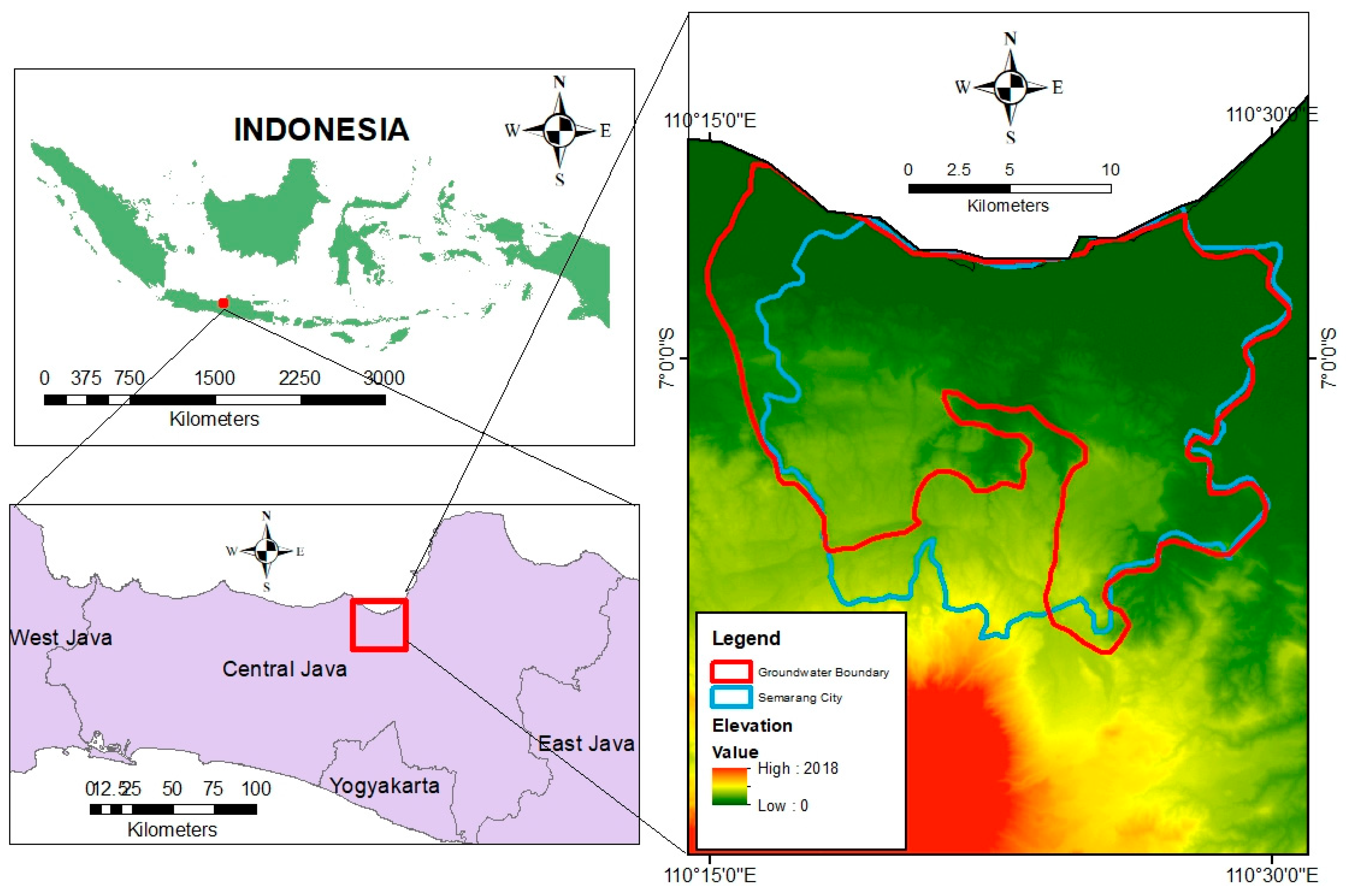
2.1. Study Area

As one of the largest cities, the fifth metropolis of Indonesia, and also the capital of the Central Java province, Semarang City has developed into one of the most important cities in Indonesia. The city has 16 districts, which extends over 109°35′–110°50′ east longitude, and 6°50′–7°10′ south latitude, as well as being located on the north coast of the Java island (Figure 1).

Semarang City has an area of 373.70 km² with a population of 1.786 million people (in 2018). The average annual population growth is 1.64% per year [25]. The northern part of Semarang City has a flat topography, which contains the lowland, coastal area at an elevation of 0.75 to 5.00 m above sea level. Infrastructure facilities in the city center include: Tanjung Emas Port, Tawang and Poncol Railway Stations, Jenderal Ahmad Yani Airport, and government offices. There are also high-density residential buildings, as well as industrial and commercial activities. On the other hand, the southern part of Semarang City consists mainly of highlands with higher altitudes up to 348 m above sea level, whose land use is essentially for agriculture, housing, public services, education, tourism, and open spaces [26].

As a consequence of excessive pumping of groundwater together with its location in a coastal area that has an alluvial soil structure, the north and northeast of Semarang City have long suffered a side effect in the form of subsidence, making the area more prone to flooding. In 2010, the regional assembly of the Parliament of Semarang as well as the Mayor of Semarang drew up a regional ordinance on spatial plans for 2011–2031. One strategy of the spatial plans is to develop an infrastructure system for water resources so as to reduce the reliance on groundwater use. Areas with restrictions on groundwater abstraction are Tugu District, West Semarang District, North Semarang District, Central Semarang District, South Semarang District, East Semarang District, Genuk District, Pedurungan District, and Gayamsari District [27].

There are two different types of wells in Semarang City: dug wells (shallow wells) and boreholes (deep wells). Dug wells usually are installed by the local residents for their daily needs, while boreholes are utilized for industrial wells. The deep wells are in a confined aquifer with a depth varying between 60 and 180 m. The registration of the number of wells used in Semarang City date back to 1900. Figure 2 shows the registered number of groundwater wells and their production capacity, which also explicitly indicates that the number and production capacity of wells are increasing every year [28,29,30,31]. Since 1999, both the number of wells and their production capacity have increased rapidly. Deep wells in the Semarang groundwater basin are mainly scattered to the north and northeast of Semarang City, and those deep wells are extensively used for industry.

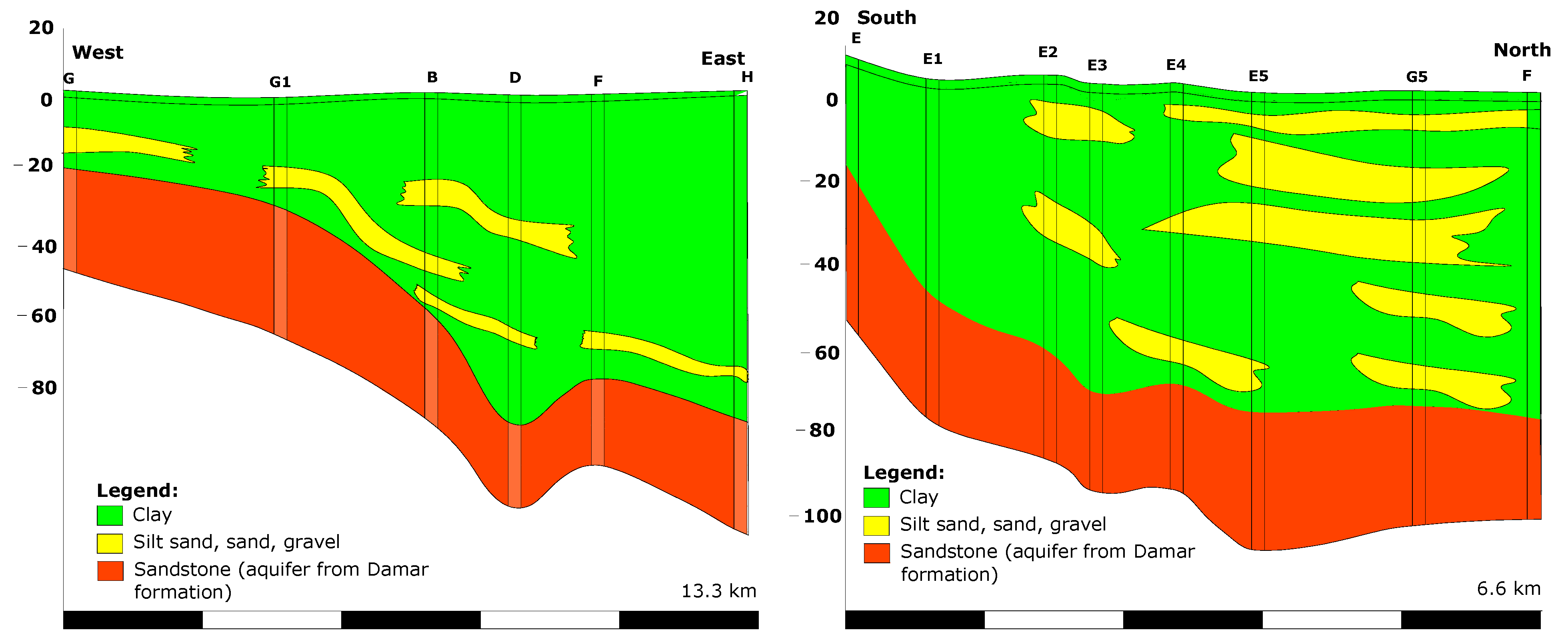
2.2. Geology, Hydrology, and Hydrogeology

The hydrogeological conceptual model is the basis for groundwater modeling since the former provides a brief but accurate description of the geological unit and groundwater flow system [32], which contains different components, e.g., the hydrogeological system, the groundwater flow field, and the water budget [24]. The input physical parameters for the Semarang groundwater model include the boundary condition of the groundwater basin, the recharge from the hydrological analysis, as well as the hydrogeological data from aquifers, rivers, and wells.

Geologically, the northern part of Semarang City is an alluvium Holocene formation, the central part of Semarang City is the Damar and Kaligetas (Pliocene) formation, and the southern part of Semarang is the Kaligetas volcanic (Pleistocene) formation [33]. The low coastal plain in the north of Semarang City comprises alluvial deposits of river, marine, and lake deposits (Qa), while the southern hills consist of the Quartenary volcanic rocks and Tertiary sedimentary formations. Based on the regional geological map (Figure 3), the stratigraphy of Semarang City, from the oldest to the youngest order, consists of the Kerek formation (Tmk), Kalibeng formation (Tmpk), Kaligetas formation (Qpkg), Damar formation (Qtd), undifferentiated volcanic rocks (Qv), and alluvial deposit (Qa). The Kerek formation (Tmk) is composed of alternating claystone, marl, and limestone. Meanwhile, the Kalibeng formation (Tmpk) consists of marl intercalated with tuffaceous sandstone and limestone. The Kaligetas formation (Qpkg) is composed of breccia, lava flows, tuffaceous sandstone, whereas the Damar formation (Qtd) is composed of tuffaceous sandstone, conglomerates, and volcanic breccia. The alluvial deposit (Qa) consists of clay, silt, sand, and gravels deposited in terrestrial and marine conditions. Geological structures in Semarang City include the thrust fault at the southern part and the strike-slip fault parallel to the Garang River [34,35].

The groundwater basin of Semarang City belongs to one part of the Semarang-Demak groundwater basin. The Semarang groundwater basin is bounded by a no-flow boundary from impermeable rock and reverse faulting in some southern parts of Semarang City, a groundwater divide boundary at the southwest (extending from the south towards the north), and a constant head boundary accounting for sea and rivers in the north, west, and east of Semarang City [28].

Hydrogeological data are essential to capture the hydrogeological characteristics of an area, by which the fluid flow in aquifer layers can be quantitatively evaluated through numerical modeling. Hydrogeological data were obtained from the geo-electric field survey conducted in February 2019 as well as the borehole data that were collected from several sources, including from the Balai Besar Wilayah Sungai (BBWS) and Pemali-Juana [31]. The geological stratum of the Semarang groundwater basin is shown in Figure 4.

Hydrologically, Semarang City is divided into 6 watersheds from west to east. They are Blorong, West Mangkang (Mangkang Barat), East Mangkang (Mangkang Timur), Garang, East Kanal (Kanal Timur), and Babon. There are four major rivers flowing in Semarang City: the Mangkang Barat/West Mangkang River, Mangkang Timur/East Mangkang River, Garang River, and Canal Timur/East Canal River. As other cities in Indonesia, Semarang City has two distinct seasons, i.e., the dry season and the wet (rainy) season. The dry season lasts from April to September, while the period from October to March is the rainy season. The mean annual temperature and humidity in Semarang City are 28.08 °C and 76.61%, respectively. The annual rainfall in Semarang City varies from 1500 to 3000 mm. The rainfall during the wet months is a source of groundwater recharge [36], but the heavy rainfall frequently causes problems of river overflow and flooding.

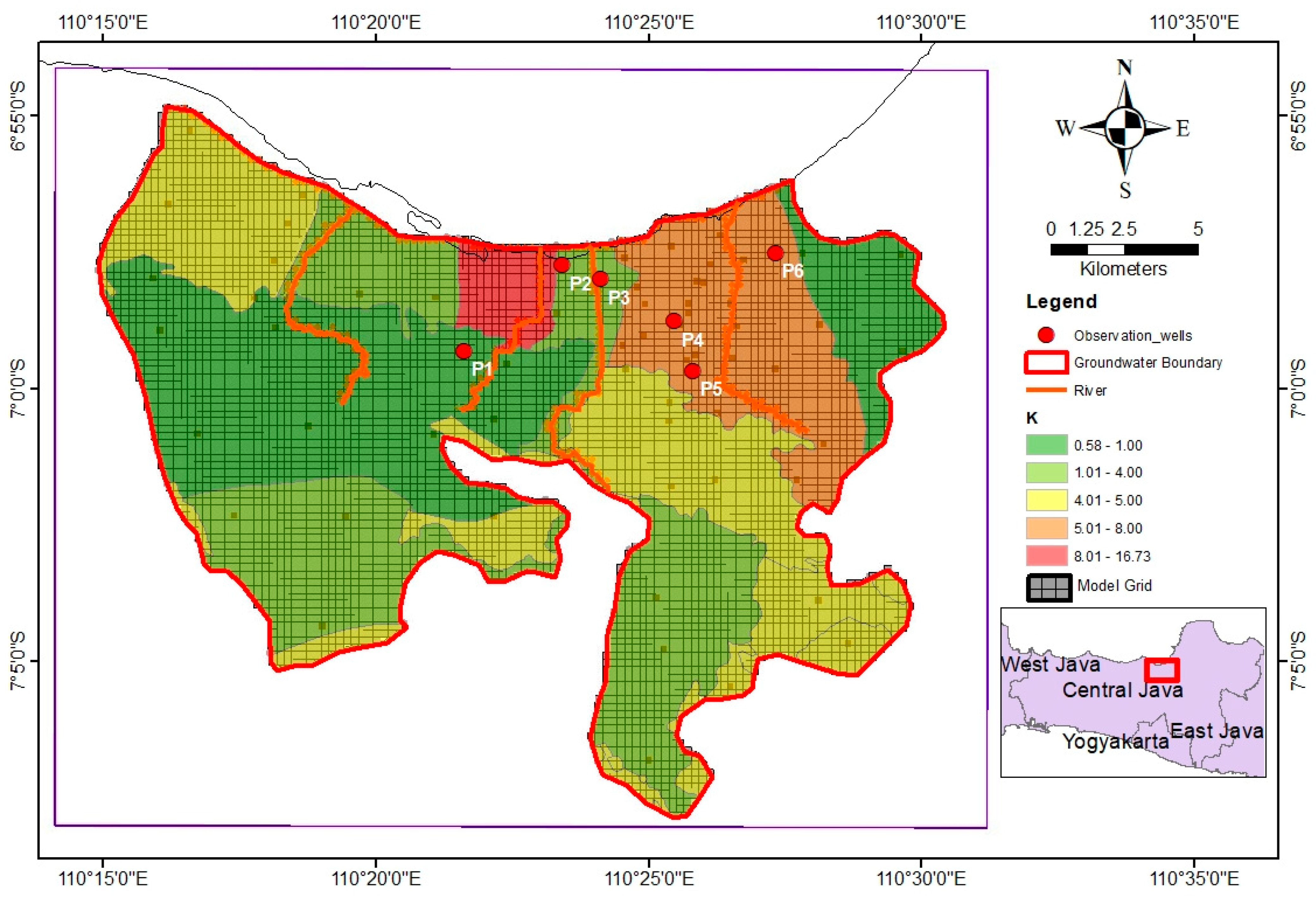
2.3. Groundwater Modeling

Geophysical experiments are usually conducted to explore the formation of groundwater system. Therefore, a wide range of data related to pumping operations and soil parameters is required, which makes it expensive and time-consuming. Groundwater numerical modeling holds great promise for a better understanding of the groundwater system and an effective implementation of groundwater management.

Numerical modeling can provide an accurate, quantitative description of groundwater behaviors, which can serve as the guidance and professionalism for structuring better strategic management. MODFLOW is a computer program for three-dimensional modeling of groundwater movement through porous materials [37]. The first MODFLOW program was documented and written in FORTRAN ’66 [38] by the United States Geological Survey (USGS). In the early 1990s, MODFLOW had been widely used all over the world since then. In the early 2000s, some additions were made for estimating transport parameters. MODFLOW-2000 possesses the features and capabilities of the groundwater flow and transport, as well as parameter estimation functionality [39] with integration of user-friendly interfaces.

According to Darcy’s Law, three-dimensional groundwater movement can be described by the partial differential equation as follows [38]:

$$\frac{\partial }{\partial x}\left(K_{xx}\frac{\partial h}{\partial x}\right)+\frac{\partial }{\partial y}\left(K_{yy}\frac{\partial h}{\partial x}\right)+\frac{\partial }{\partial z}\left(K_{zz}\frac{\partial h}{\partial z}\right)-W=S_s\frac{\partial h}{\partial t}$$

(1)

where:

x, y, z = Cartesian coordinates in x, y, and z directions;

K_xx, K_yy, K_zz = components of the hydraulic conductivity tensor in the x, y, and z direction;

W = volumetric flux per unit volume of sources and (or) sinks of water;

S_s = specific storage;

h = hydraulic head.

Hydrogeological modeling is often conducted using an integrated approach. A hydrostratigraphic unit (HSU) in Semarang City has been previously delineated [40]. It consists of two hydrogeological systems, unconfined and confined aquifers. An unconfined aquifer is found in alluvial deposits near the surface with water table fluctuating with seasonal precipitation. Salinization of the unconfined aquifer has occurred in the coastal lowland area, making the water unsuitable for daily use [41]. There are two confined aquifer systems in the study area, the Quartenary deposit aquifer and the Damar formation aquifer [40]. The Quartenary deposit aquifer consists of the Garang delta aquifer and Quartenary marine aquifer. Both are within the alluvial deposit, flowing in an intergranular system. The Garang delta aquifer has freshwater quality and the Quartenary marine aquifer contains brackish water as a result of its deposition [40,42]. The Quartenary aquifer system forms as lenses within the alluvial deposit, yielding lesser quantity of groundwater than the intergranular system of the volcanic sedimentary rocks of the Damar formation. This study thus focused on the problem as to the groundwater exploitation of the Damar formation aquifer, which has caused an extensive cone of depression of the piezometric water table. Groundwater from the Damar formation aquifer flows from the mountainous region in the south to the lowland in the north. It can be seen that the cone of depression formed in the north coastal plain in 1984, and widened southward in 2010.

2.4. Conceptual Model

A groundwater model for the Semarang groundwater basin was rigorously established, as presented in Figure 5. In this study, each cell has a size of 250 m × 250 m in the horizontal direction, while the height of each cell is equal to the depth of the soil layer in the vertical direction. The computation grid consists of 126 and 104 cells along the x and y axes, respectively. According to the geological investigation as shown in Figure 4, the z-axis of the model consists of three layers, i.e., top soil in the first layer, clay in the second layer, and sandstone in the third layer. Due to the importance of hydrogeological elements, the Semarang aquifer is divided into 21 hydrogeological polygon zones, with the aquifer permeability in the Semarang groundwater basin ranging from 0.57 to 16.73 m/day, the transmissivity taking the value of 27.6 to 210.8 m²/day, and a specific storage coefficient being about 5 × 10⁻⁶ (1/m) [28]. In addition, four rivers should be represented in the model: Mangkang Barat/West Mangkang River, Mangkang Timur/East Mangkang River, Garang River, and Canal Timur/East Canal River. The specified boundary condition (IBOUND) is prescribed for these river flows.

There are 54 observation wells that are scattered around Semarang City. Unfortunately, many recorded data of observation wells are missing, which cannot be served for the calibration of the numerical modeling. There are six observation wells, i.e., Prawiro Jaya Baru (P1), PRPP (P2), SMKN 10 (P3), Wot Gandul (P4), Santika Hotel (P5), and LIK Kaligawe (P6), which currently contain sufficient data to be suitable for the calibration of the numerical model in Semarang City. Figure 5 shows the grid map, the hydrogeological polygon zones, the river map, and the position of observation wells.

The other input parameters for the numerical model also comprise tidal data from the north of Semarang City as high as 1.07 m, the average precipitation (from 1970 to 1990) as the recharge rate in the steady-state flow simulation, and the precipitation (from 1990 to 2010) as the recharge rate in the transient flow simulation. The sources that provide the data entry for the groundwater numerical model in Semarang City used in MODFLOW are given in

Table 1. Data source for the groundwater modeling in Semarang City used in MODFLOW.

Data	Sources
DEM (Digital Elevation Model)	Resolution 0.27 arc-sec ≈ 8.325 m, source: DEMNAS Indonesia
Rainfall data	Water Resource Agency, Public Work Department of Indonesia
Soil properties	Mining and Energy Agency of Central Java Province
Wells location and discharge	Mining and Energy Agency of Central Java Province
Observation wells location and groundwater level	Center for Groundwater and Environmental Geology, Ministry of Energy and Mineral Resources
Hydrogeological data:
1. Borehole data	1. BBWS Pemali—Juana, Ministry of Public Work
	2. Mining and Energy Agency of Central Java Province
2. Geoelectrical data	1. Primary data from field survey
	2. Secondary data from the Department of Geology, Diponegoro University

.

3. Results and Discussion

3.1. Error Measurement of Models

The groundwater numerical modeling in this study was performed under the steady-state and transient flow conditions. For calibration process, the data associated with recorded hydraulic head from the six observation wells are imported into the model. To minimize the difference between the recorded head and the estimated head obtained from the simulation, a trial and error method is used. The quality of the calibration is systematically evaluated by the root mean square error (RMSE) and the coefficient of determination (R²).

3.1.1. Root Mean Square Error (RMSE)

Root Mean Square Error (RMSE), also known as the root mean square deviation (RMSD), has been widely used to measure the error of a numerical model, which represents the absolute error between the observed and simulated values [43]. A value of 0 indicates a perfect fit to the data. The closer to 0, the smaller the error, and the more accurate the simulation result. RMSE can be calculated as

$$RMSE=\sqrt{\frac{{{\displaystyle \sum }}_{t=1}^n{\left(H_0^t-H_p^t\right)}^2}{n}}$$

(2)

where:

$H_0^t$ = observed data at time t;

$H_p^t$ = predicted data at time t;

n = number of data.

3.1.2. Coefficient of Determination (R²)

The coefficient of determination, also known as R-squared, is used to assess the suitability of a model based on the recorded data obtained from the observation wells [44,45]. The coefficient of determination has a range of values from 0 to 1. The value of R² that is close to the value 1 indicates a near-perfect relationship between the model and recorded data [46,47]. This coefficient is determined by [47]

$$R^2=1-\frac{{{\displaystyle \sum }}_{i-1}^n{\left(H_0-H_p\right)}^2}{{{\displaystyle \sum }}_{i-1}^n{\left(H_0-\overline{H}\right)}^2}$$

(3)

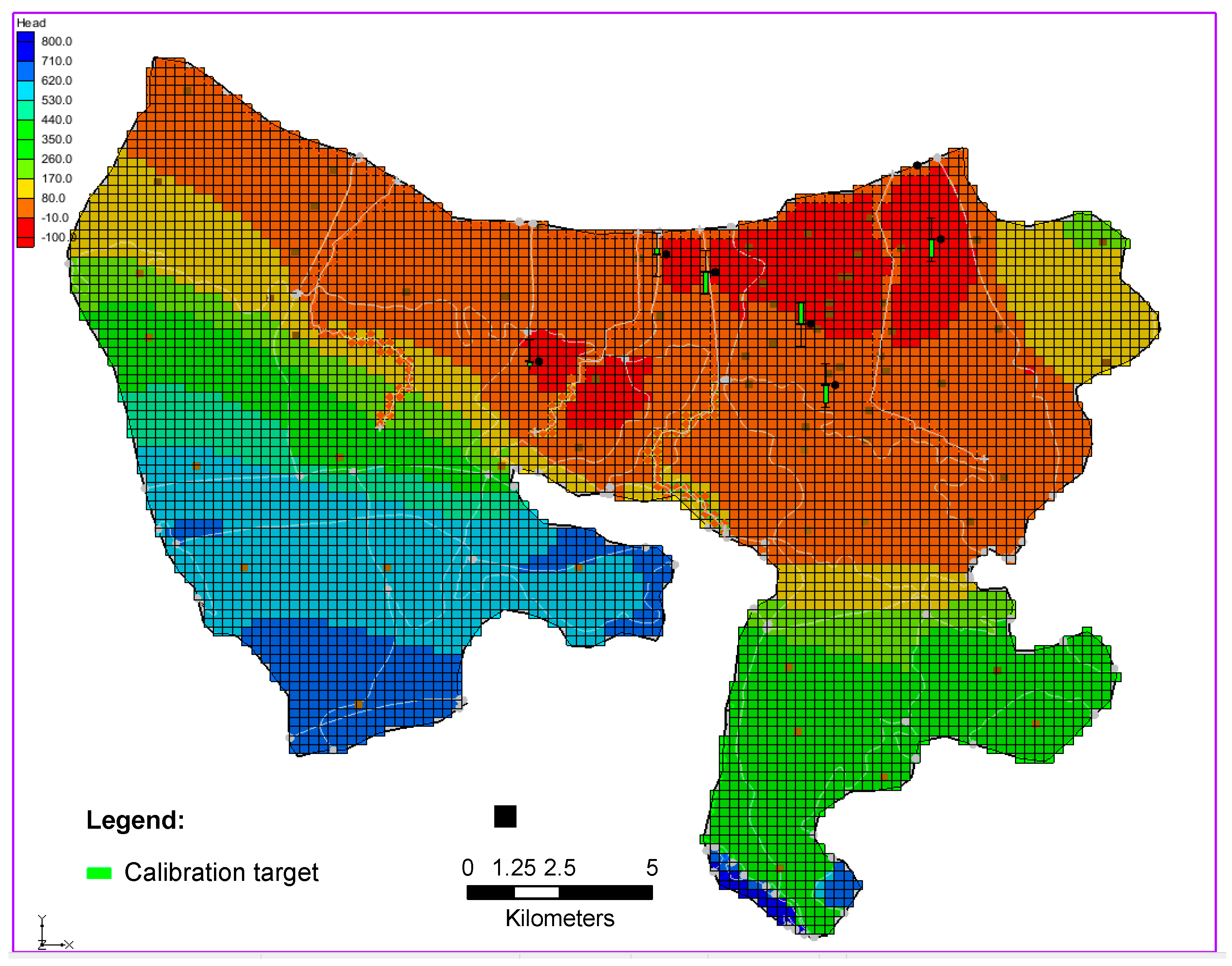
3.2. Steady-State Flow Simulation

The steady-state flow simulation was used to ensure the rationality of the inputted hydrogeological parameters and later used as the initial condition for the transient flow simulation. In the steady-state flow simulation, the values of optimal input parameters for all grids, such as recharge and hydraulic conductivity, are determined to make the computed head in the model accurately capture the observation head. In the current study, the period of 1970 to 1990 was used for the steady-state flow simulation to obtain the predicted head.

For calibration process, the head discrepancy is set to 1 m with 95% confidence interval to ensure that the predicted head from numerical simulations is not significantly different from the observed head. The head discrepancy represents the difference between the observed head and the predicted head, and can be used as a calibration criterion [48], which is illustrated using a colored bar. If the bar is green, the calibration is within the allowed target. If the error value is outside the target, but less than 200%, the bar is yellow. However, if the error value is more than 200%, the bar is marked as red [48]. The calibration is accepted if the estimated error interval is less than the head discrepancy, and simultaneously is also supported by a sufficiently small RMSE value. The comparison of the observed and predicted heads is shown in Figure 6 and

Table 2. Results of the steady-state flow simulation.

Name	Recorded Head (m)	Predicted Head (m)
Prawiro Jaya Baru (P1)	4.475	4.268
PRPP (P2)	−6.380	−6.104
SMKN 10 (P3)	−6.328	−7.252
Wot Gandul (P4)	−7.746	−6.781
Santika Hotel (P5)	5.802	4.971
LIK Kaligawe (P6)	−11.879	−12.662

, where the RMSE values for the six observation wells are also given.

Figure 6 reveals that all of the colored bars at the six observation wells are green. Evidently, this implies that our numerical simulation for the steady-state flow condition is within the calibration target. Furthermore,

Table 3. Total RMSE and R² for the transient flow simulation.

Name	RMSE (m)	R2
Prawiro Jaya Baru (P1)	0.400	0.600
PRPP (P2)	3.500	0.831
SMKN 10 (P3)	0.733	0.962
Wot Gandul (P4)	1.429	0.808
Santika Hotel (P5)	0.806	0.610
LIK Kaligawe (P6)	1.729	0.989

shows the recorded head and predicted head at these six observation wells. The RMSE at the six observation wells is 0.731 m, physically indicating that the value predicted by the model is in quite good agreement with the observed value.

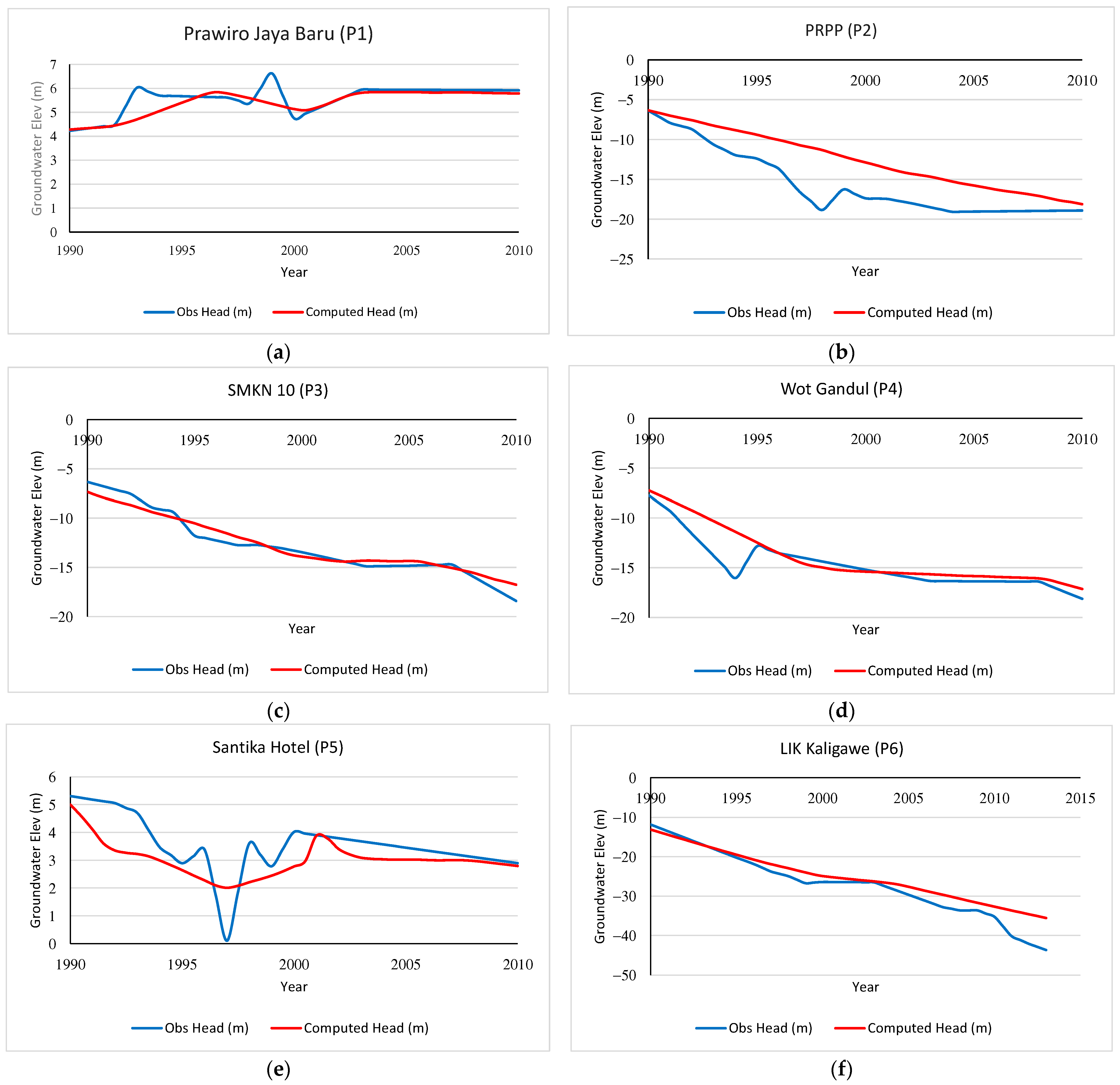
3.3. Transient Flow Simulation

The result of the steady-state flow simulation provides the rational, accurate initial condition for the next phase of the transient flow simulation. The calibration period for the latter simulation is from 1990 to 2005 and a validation period is from 2005 to 2010. As done previously for the steady-state flow simulation, the same head discrepancy (i.e., 1 m) with 95% confidence interval is stipulated for the transient flow simulation. Comparison of the estimated head (in red) with the recorded head (in blue) is graphically presented in Figure 7 from 1990 to 2010 at the six observation wells. In addition, the total RMSE value together with the coefficient of determination (R²) are calculated to illustrate the performance of our numerical model for the transient flow simulation, which are listed in Table 3.

As an aside, we indeed note from Table 3 that P2 has the largest RMSE value, while P1 and P5 have small R² values. The PRPP (P2) point had the highest RMSE of 3.5 m. As a result, we are concentrating on investigating at this point. We analyze that this is due to the boundary condition in the form of tides as high as 1.07 m. The existence of a boundary condition that is very close to the observation point P2 appears to interfere with the conceptual model, resulting in a fairly large RMSE value, whereas it gives a small RMSE value for other observation points that are far away from the boundary conditions. The small value of R² at P1 and P5 is mainly due to a sudden drop in the groundwater level that occurs at a certain year, as shown in Figure 7. This decline is beyond the existing trend. As we note, this was generated by the alteration of observation equipment in that year. Evidently, RMSE and R² values thus produce less robust results since there are outlier data as a result of instrument error [49,50].

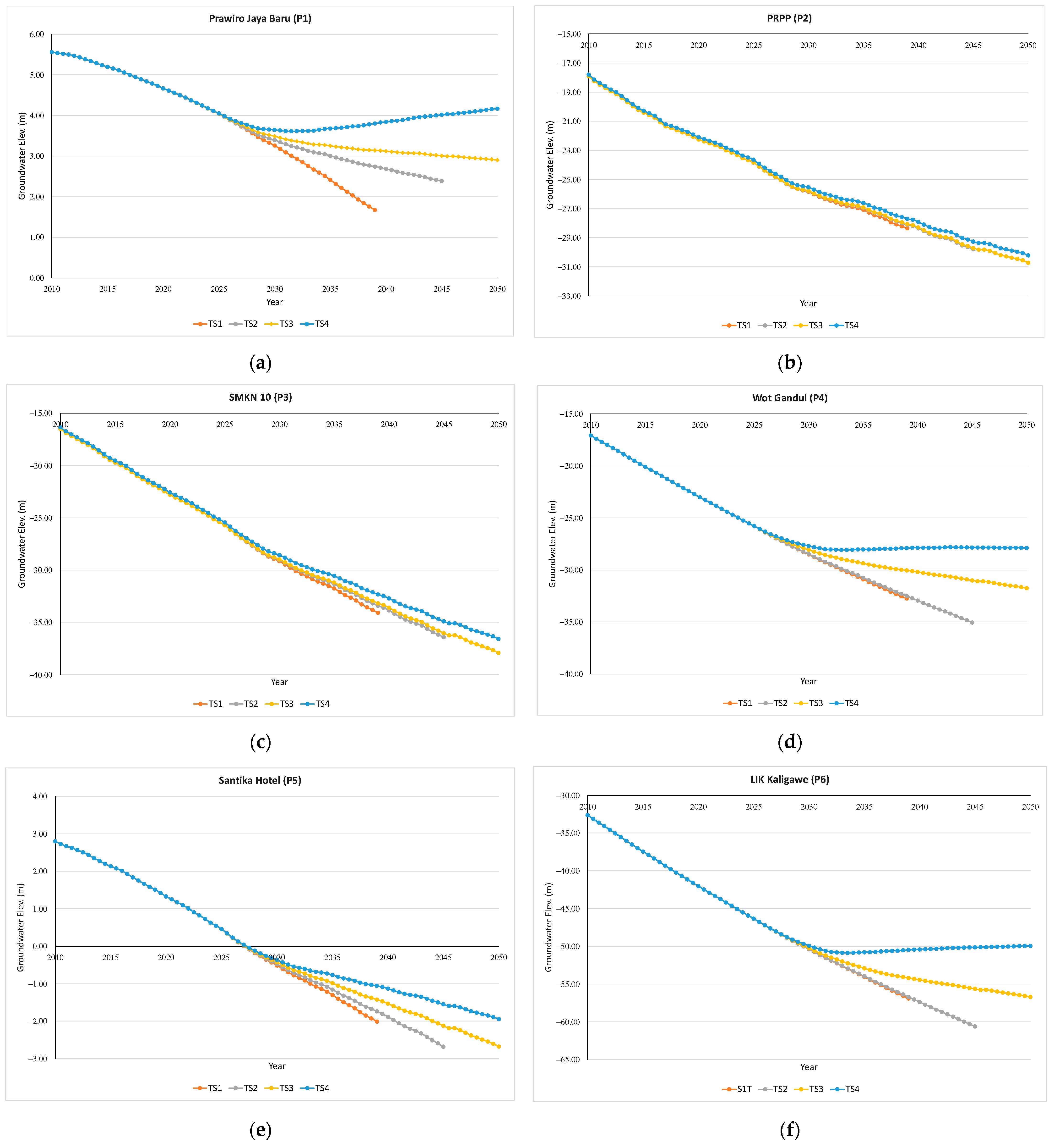
3.4. Scenario Design

After calibrating and validating the model, four scenarios that reflect potential management strategies are investigated. To achieve this, we revisit Figure 2, which provides the information as to the number of the registered deep wells and their production capacity in Semarang City. A regression analysis can be undertaken to show that the equation describing the trendline of production capacity can be evaluated by y = 738.1e^0.0465x, while that describing the trendline of the number of the registered deep wells can be determined to be y = 9.3222e^0.0422x, as demonstrated in Figure 8.

The first scenario (TS1) is a direct projection of the future water consumption from 2010 to 2050, which is calculated straightforwardly based on the two trendline equations gained in Figure 8 without any management measure. The second (TS2), third (TS3), and fourth (TS4) scenarios are the ones with the values computed from the two trendline equations for the period of 2010 to 2024, but from 2025 to 2050, TS2, TS3, and TS4 respectively represent different measures adopted to restore the groundwater level. A flat line is prescribed in the second scenario (TS2) for the registered deep wells and their production capacity between 2025 and 2050, physically indicating that the measure is proposed to prohibit the development of additional wells and groundwater production in this period. The third scenario (TS3) characterizes a more ambitious measure that is planned to reduce the number of the registered deep wells and their production capacity by 5% annually from 2025 to 2034 and then maintains them from 2035 to 2050. A same measure as the third scenario but with 10% reduction is formulated instead as the fourth scenario (TS4).

The results obtained from our numerical simulation for these four scenarios in the six observation wells are graphically presented in Figure 9. Apparently, it can be seen from Figure 9 that if we do not take any control measures, the groundwater resource will be fully depleted in these six wells approximately after 2040 and 2045 under the scenario of TS1 and TS2, respectively. Figure 9 also indicates that the control measures (TS3 and TS4) we proposed indeed have a significant effect on groundwater restoration for Prawiro Jaya Baru (P1), Wot Gandul (P4), and LIK Kaligawe (P6). However, the groundwater level at the location of PRPP (P2), SMKN 10 (P3), and Santika Hotel (P5) in 2050 is still lower than that in 2025, even though these control measures are implemented. This implies that the groundwater resources have been extensively overexploited at these three wells; therefore, it needs more aggressive (i.e., more than 10% reduction rate) control measures. The groundwater level almost returns back to that in 2025 at the Prawiro Jaya Baru (P1) observation well under the TS4 scenario.

4. Conclusions

Overexploiting freshwater aquifers has caused a gradual decline in the groundwater level. In the current study, Semarang City was investigated for the abstraction of groundwater in deep wells due to the expansion of industrial facilities. A numerical MODFLOW model for Semarang City was developed to examine the physics and dynamics of groundwater flow and to evaluate the impact of groundwater extraction. The calibration is delicately performed under two very different flow conditions of the steady and transient states at six observation wells. The mean square error and the coefficient of determination are used as quantitative indicators to assess the reliability of the model.

Although there are only the limited number of observation wells that have brought the complexity in calibrating and validating the hydrological parameters and recharge rates, especially in the southern part of Semarang City, MODFLOW has been demonstrated as a powerful numerical model. Combination of MODFLOW and spatial analysis indeed provides valuable and robust reference for groundwater resources management. However, to aid the formulation of better groundwater management plans, it should increase the number of new observation wells or reactivate the number of existing observation wells, especially in the western and southern parts of Semarang City.

Four management strategies are then presented in the current study in an attempt to achieve sustainability of the groundwater resources in relation to their excessive extraction caused by rapid urbanization in Semarang City. The result shows that even though 10% reduction in the development of the deep wells and their production capacity is implemented from 2035 to 2050 (TS4), only the groundwater level in Prawiro Jaya Baru (P1) can restore back to that recorded in 2025 among these 6 observation wells. The declines in groundwater level can be essentially controlled in Wot Gandul (P4) and LIK Kaligawe (P6). However, in PRPP (P2), SMKN 10 (P3), and Santika Hotel (P5), the groundwater level still continues to drop and is even lower by 20 m than that in 2010 in SMKN 10 (P3). Therefore, to fulfill sustainable groundwater management that meets future beneficial uses without leading to unacceptable environmental consequences, such as land subsidence and, in turn, susceptibility to flooding, in Semarang City, it should strengthen administrative regulation with a systematic registration of pumping wells, implement abstraction control policy, and even place restrictions on future groundwater use, in quantity, by more than 10%, as indicated in the current study. Reduction of the grid size together with consideration of land use change and human behavior towards groundwater use are highly recommended for further studies. Moreover, due to the excessive exploitation of groundwater, it is strongly recommended to conduct further research as to the effect of groundwater resources overexploitation on land subsidence.

References

1. United Nations. Available online: https://www.un.org/en/development/desa/population/theme/urbanization/index.asp (accessed on 28 October 2020).
2. Bradley, R.M.; Weeraratne, S.; Mediwake, T.M.M. Water use projections in developing countries. J. Am. Water Work. Assoc. 2002, 94, 52–63. [Google Scholar] [CrossRef]
3. McDonald, R.I.; Green, P.; Balk, D.; Fekete, B.M.; Revenga, C.; Todd, M.; Montgomery, M. Urban growth, climate change, and freshwater availability. Proc. Natl. Acad. Sci. USA 2011, 108, 6312–6317. [Google Scholar] [CrossRef] [PubMed] [Green Version]
4. McDonald, R.I.; Weber, K.; Padowski, J.; Flörke, M.; Schneider, C.; Green, P.A.; Gleeson, T.; Eckman, S.; Lehner, B.; Balk, D.; et al. Water on an urban planet: Urbanization and the reach of urban water infrastructure. Glob. Environ. Chang. 2014, 27, 96–105. [Google Scholar] [CrossRef] [Green Version]
5. McGrane, S.J. Impacts of urbanisation on hydrological and water quality dynamics, and urban water management: A review. Hydrol. Sci. J. 2016, 61, 2295–2311. [Google Scholar] [CrossRef]
6. Semarang City’s Central Statistics Agency. Available online: https://semarangkota.bps.go.id/ (accessed on 28 October 2020).
7. Gorelick, S.M.; Zheng, C. Global change and the groundwater management challenge. Water Resour. Res. 2015, 51, 3031–3051. [Google Scholar] [CrossRef]
8. Braga, A.C.R.; Serrao-Neumann, S.; de Oliveira Galvão, C. Groundwater Management in Coastal Areas through Landscape Scale Planning: A Systematic Literature Review. Environ. Manag. 2020, 65, 321–333. [Google Scholar] [CrossRef] [PubMed]
9. Morris, B.L.; Lawrence, A.R.L.; Chilton, P.J.C.; Adams, B.; Calow, R.C.; Klinck, B.A. Groundwater and Its Susceptibility to Degradation: A Global Assessment of the Problem and Options for Management; Early Warning and Assessment Report Series, RS. 03-3; United Nations Environment Programme: Nairobi, Kenya, 2003. [Google Scholar]
10. Margat, J.; van der Gun, J. Groundwater around the World: A Geographic Synopsis; CRC Press, Taylor & Francis Group: Boca Raton, FL, USA, 2013; ISBN 978-0-203-77214-0. [Google Scholar]
11. Turner, S.W.D.; Hejazi, M.; Yonkofski, C.; Kim, S.H.; Kyle, P. Influence of Groundwater Extraction Costs and Resource Depletion Limits on Simulated Global Nonrenewable Water Withdrawals Over the Twenty-First Century. Earth’s Future 2019, 7, 123–135. [Google Scholar] [CrossRef] [Green Version]
12. Custodio, E.; Albiac, J.; Cermerón, M.; Hernández, M.; Llamas, M.R.; Sahuquillo, A. Groundwater mining: Benefits, problems and consequences in Spain. Sustain. Water Resour. Manag. 2017, 3, 213–226. [Google Scholar] [CrossRef]
13. Molle, F.; López-Gunn, E.; van Steenbergen, F. The local and national politics of groundwater overexploitation. Water Altern. 2018, 11, 445–457. [Google Scholar]
14. Satyaji Rao, Y.R.; Siva Prasad, Y. Groundwater flow modeling—A tool for water resources management in the khondalite and sandstone formations. Groundw. Sustain. Dev. 2020, 11, 100454. [Google Scholar] [CrossRef]
15. Gonçalves, R.D.; Teramoto, E.H.; Chang, H.K. Regional groundwater modeling of the guarani aquifer system. Water 2020, 12, 2323. [Google Scholar] [CrossRef]
16. Pastore, N.; Cherubini, C.; Doglioni, A.; Giasi, C.I.; Simeone, V. Modelling of the Complex Groundwater Level Dynamics during Episodic Rainfall Events of a Surficial Aquifer in Southern Italy. Water 2020, 12, 2916. [Google Scholar] [CrossRef]
17. Drias, T.; Khedidja, A.; Belloula, M.; Badraddine, S.; Saibi, H. Groundwater modelling of the Tebessa-Morsott alluvial aquifer (northeastern Algeria): A geostatistical approach. Groundw. Sustain. Dev. 2020, 11, 100444. [Google Scholar] [CrossRef]
18. Gogu, R.C.; Carabin, G.; Hallet, V.; Peters, V.; Dassargues, A. GIS-based hydrogeological databases and groundwater modelling. Hydrogeol. J. 2001, 9, 555–569. [Google Scholar] [CrossRef]
19. Dawoud, M.A.; Darwish, M.M.; El-Kady, M.M. GIS-based groundwater management model for Western Nile Delta. Water Resour. Manag. 2005, 19, 585–604. [Google Scholar] [CrossRef]
20. Singh, A. Groundwater modelling for the assessment of water management alternatives. J. Hydrol. 2013, 481, 220–229. [Google Scholar] [CrossRef]
21. Rojas, R.; Kahunde, S.; Peeters, L.; Batelaan, O.; Feyen, L.; Dassargues, A. Application of a multimodel approach to account for conceptual model and scenario uncertainties in groundwater modelling. J. Hydrol. 2010, 394, 416–435. [Google Scholar] [CrossRef] [Green Version]
22. Batelaan, O.; De Smedt, F.; Triest, L. Regional groundwater discharge: Phreatophyte mapping, groundwater modelling and impact analysis of land-use change. J. Hydrol. 2003, 275, 86–108. [Google Scholar] [CrossRef]
23. Boufekane, A.; Saibi, H.; Benlaoukli, B.; Saighi, O. Scenario modeling of the groundwater in a coastal aquifer (Jijel plain area, Algeria). Arab. J. Geosci. 2019, 12, 1–14. [Google Scholar] [CrossRef]
24. El Alfy, M. Numerical groundwater modelling as an effective tool for management of water resources in arid areas. Hydrol. Sci. J. 2014, 59, 1259–1274. [Google Scholar] [CrossRef]
25. Semarang Central Bureau of Statistic. Badan Pusat Statistik Semarang City in Figures 2019 (Kota Semarang Dalam Angka Tahun 2019); Semarang Central Bureau of Statistic: Semarang, Indonesia, 2019; pp. 1–346. [Google Scholar]
26. Semarang City Government. Urban Planning of Semarang City 2011–2031; Semarang City Government: Semarang, Indonesia, 2011.
27. Pemerintah Kota Semarang. Spatial Plans of Semarang City 2011–2031; Pemerintah Kota Semarang: Semarang, Indonesia, 2010; pp. 1–30, (In Bahasa Indonesia). [Google Scholar]