
A Comparative Investigation of Various Pedotransfer Functions and Their Impact on Hydrological Simulations


1
Department of Physical Geography, Faculty VI, University of Trier, Universitätsring 12, 54296 Trier, Germany
2
TUM Department of Civil, Geo and Environmental Engineering, Technical University of Munich (TUM), Arcisstrasse 21, 80333 München, Germany
*
Author to whom correspondence should be addressed.
Water 2021, 13(10), 1401; https://doi.org/10.3390/w13101401
Submission received: 22 April 2021
/
Revised: 13 May 2021
/
Accepted: 14 May 2021
/
Published: 17 May 2021
(This article belongs to the Special Issue Recent Progress in Linking Soil Science and Hydrology)
Abstract
:Soil hydraulic properties, which are basically saturated and unsaturated hydraulic conductivity and water retention characteristics, remarkably control the main hydrological processes in catchments. Thus, adequate parameterization of soils is one of the most important tasks in physically based catchment modeling. To estimate these properties, the choice of the PTFs in a hydrological model is often made without taking the runoff characteristics of the catchment into consideration. Therefore, this study introduces a methodology to analyze the sensitivity of a catchment water balance model to the choice of the PTF. To do so, we define 11 scenarios including different combinations of PTFs to estimate the van Genuchten parameters and saturated hydraulic conductivity. We use a calibrated/validated hydrological model (WaSiM-ETH) as a baseline scenario. By altering the underlying PTFs, the effects on the hydraulic properties are quantified. Moreover, we analyze the resulting changes in the spatial/temporal variation of the total runoff and in particular, the runoff components at the catchment outlet. Results reveal that the water distribution in the hydrologic system varies considerably amongst different PTFs, and the water balance components are highly sensitive to the spatial structure of soil hydraulic properties. It is recommended that models be tested by careful consideration of PTFs and orienting the soil parameterization more towards representing a plausible hydrological behavior rather than focusing on matching the calibration data.
1. Introduction
The projected future changes in the land-use, climate, and water cycle lead to an increasing demand for modeling approaches and frameworks for the simulation of hydrological processes at local and regional scale of water resource management. Therefore, a well parameterized and calibrated physically based hydrological model, which is capable of realistically reproducing the behavior of the hydrologic system, is considered particularly important in order to provide decision makers in water resources management with reliable predictions [1]. Soil hydraulic properties have a major impact on the main hydrological processes in catchment areas [2,3]. Therefore, information on these soil properties plays a key role in water balance modeling, and an adequate parameterization of soils is one of the most important tasks in physically based catchment modeling [4,5]. Richard’s equation [6], which describes the water flow in unsaturated soil by combining the Darcy–Buckingham law with the continuity equation, is the dominant concept of soil physics in hydrological textbooks [7,8,9]. It can be considered as the fundamental concept underlying “physically-based” hydrological models [10]. To solve this equation, information on soil hydraulic properties is required [11].
Parameters of soil properties are usually measured as point observations at small scales. However, water balance modeling in catchments requires parameter values at larger spatial scales such as grid cells or the entire catchment [12]. The Richard’s equation is parameterized by either observed soil properties (i.e., measured relations of soil water content and matric potential) or constitutive equations such as the Gardner–Russo model [13], the Brooks-Corey model [13], or the Mualem–van Genuchten model [14,15]. These empirical models represent a basic hydro-physical characteristic of the soil: the relation between soil water content and matric potential [16].
Among the empirical models developed to parameterize the water flow in unsaturated soils, the traditional van Genuchten parameterization [15] has evolved to a de facto standard and is widely used because of its higher degree of fit to observed soil water retention data [17]. Nevertheless, to practically apply this model, obtaining its unknown empirical fitting parameters based on known experimental data (namely, a measured soil water retention curve) is essential. Moreover, at larger spatial scales, such as those of catchment models, direct measurements are not feasible due to the area coverage and the heterogeneity of the soil properties. Therefore, various methods have been developed to determine the van Genuchten parameters, and subsequently, the soil water retention curves using soil parameters that are easier to measure, such as texture, organic matter content, and bulk density. The term pedotransfer function (PTF) has been introduced to define these functional relationships that transfer available measurable soil properties into missing soil properties (e.g., soil hydraulic and soil chemical characteristics) [18]. The derivation of a PTF is usually based on a two-step process. First, the selected water retention function (e.g., van Genuchten) is fitted to measured water retention curves. In the second step, the parameter values determined in this process are related to the selected soil properties [17,19]. During the last three decades, soil scientists have developed a broad set of PTFs that differ with respect to:
- Applied methods (e.g., statistical regression techniques, data mining and exploration techniques);
- The underlying database of measured soil moisture retention data used to fit van Genuchten model estimates; and
- Required input parameters or predictors (e.g., grain size distribution, bulk density, organic matter content) to derive PTF.
Extensive reviews on this content were given by Pachepsky and Rawls (2004) [20]; Wösten et al. (2001) [11]; Vereecken et al. (2010) [17]; and Patil and Singh (2016) [21]. Accuracy and uncertainty of PTFs were evaluated by Schaap and Leij (1998) [22]. They showed that the performance of PTFs may depend strongly on: the data employed for calibration and evaluation, input soil properties, and different applied methods. The databases that have been used to derive PTFs show four remarkable differences:
- The measurement methods and techniques used to obtain the complete soil moisture retention characteristic in the laboratory;
- The sample size used at different pressure heads is not the same;
- Variations in the number of data points, as well as the values of pressure heads used to determine the WRC [17].
Parameterization of soil hydraulic properties should be done in such a way that the hydrological processes simulated using a water balance model match the locally observed processes [24,25]. From a modeler’s perspective, the inconsistencies in the data bases used for deriving the different PTFs complicate the evaluation of their reliability in a specific case. For instance, Vereecken et al. (1992) [26] showed that 90% of the variation in predicted moisture supply was attributed to estimation errors in hydraulic properties when using the PTFs developed by Vereecken et al. (1989, 1990) [27,28]. In another study, Chirico et al. (2010) [29] analyzed the effect of PTF prediction uncertainty on soil water balance components at the hillslope scale. They found that simulated evaporation is more affected by the PTF model error than by errors due to uncertainties in model input data. This sensitivity can result in a compensation of structural model errors by soil parameters, if no careful evaluation of the parameterization of soil hydraulic properties or the simulation of depth-dependent soil moisture content is made [30]. As a result, investigating the model behavior in response to change in the method used to estimate soil hydraulic properties, such as using different types of PTFs, is of major relevance to modelers. However, selection of PTF is usually not guided by its effect on the runoff behavior of the catchment model.
Therefore, the aim of this paper is to evaluate the impact of PTF selection on subsequent changes in the hydrological model behavior. We hypothesize that the PTF-specific soil water retention and hydraulic conductivity curves distinctly affect the water balance and runoff characteristics of the hydrological model, and the resulting differences may be related to the respective soil hydraulic properties of the study area as well as to the methodology to derive the PTF. To test the hypothesis (i) we adapted the soil parameterization in a calibrated and validated hydrological model by varying the underlying PTFs and determined the effects on the soil hydraulic properties of the catchment; and (ii) we analyzed the resulting changes in the model behavior with respect to the catchment outlet, as well as the spatial and temporal variation of the total flow and the flow components.
2. Materials and Methods
2.1. Study Area
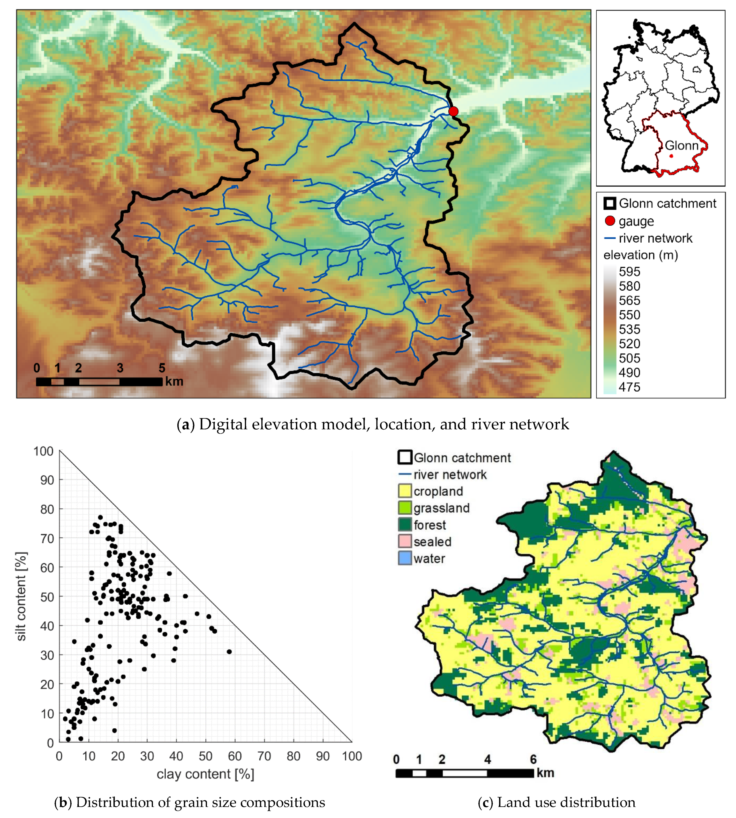
The Glonn catchment area is located in the Tertiary Molasse Hills in Bavaria, Germany. The region is characterized by a low to moderate river density and a runoff coefficient of about 35% [31]. The Molasse basin consists of deposits from the Alps, so the study area comprises a wide range of different grain size compositions. The investigated area of the Glonn catchment has a size of 104 km2 and an elevation difference of 95 m (Figure 1a), resulting in an average terrain gradient of 4.7%. The soil types were derived from the Übersichtsbodenkarte Bayern (ÜBK25) and consist mainly of Cambisol (65%) and Gley (19%), which is located near the watercourse. These grain size compositions of the soil types are displayed in Figure 1b and cover 71% of the KA5-texture classes [32] and 85% of the FAO texture classes.
The analysis of the land use distribution is based on a combination of the ATKIS dataset and the INVEKOS data and reveals an extensive agricultural use of the catchment area (Figure 1c). Cropland is the largest land use in the area with 56%, followed by forest (23%) and grassland (12%). Sealed areas (9%) are dominant at the outlet of the catchment area but are more or less evenly distributed over the entire catchment area.
Since the Glonn catchment embraces a high variety of soil and land use types, we consider this catchment to be well suited to study the general effects of different PTFs on the distribution of water in the system and on runoff generation processes.
2.2. Model Setup and Calibration
The water balance in the catchment area was investigated by applying the hydrological model WaSiM (http://www.wasim.ch, accessed on 14 May 2021). WaSiM is a distributed and deterministic model, which includes mostly physical descriptions of the hydrological processes involved. WaSiM is considered illustrative for distributed hydrological models that apply the Richard equation and PTFs to parameterize the soil hydraulic properties. The Richards approach simulates the unsaturated water flow in the soil [6]. In WaSiM, the soil is represented as layered soil columns, in which the thickness as well as the soil characteristics can be defined individually for every horizon. The description of the soil horizons comprises the water retention curve, which are described using van Genuchten parameters [15] and the saturated hydraulic conductivity (Table 1). The modeled discharge has three components (surface flow, interflow, base flow), which represent different response types (fast, intermediate, slow). The model thus allows analyzing the effects of change in soil hydraulic properties caused by multiple soil parametrizations (with different PTFs) on the runoff behavior of the catchment.
We set up the model on a spatial scale of 100 m and a temporal scale of 1 h. The required topographic spatial data (e.g., slope, flow accumulation, sub-catchment structure) were derived from TANALYS (i.e., a pre-processing tool of WaSim-ETH) [33] by performing a complex analysis of the DEM. The land use map is equivalent to the above-mentioned combination of ATKIS and INVEKOS data (Figure 1c). The soil map is derived and parameterized based on the Übersichtsbodenkarte Bayern (ÜBK25). The depth profiles of the bulk density and organic matter content of the soil types were adapted according to the overlying main land use type. For the calibration of the baseline scenario, we choose: (1) the PTF of [19] to derive the van Genuchten parameters, and (2) the KA5 [32] which contains a table for the derivation of saturated hydraulic conductivities from texture classes. The considered input time series contain precipitation, temperature, relative humidity, global radiation, and wind speed interpolated from station data.
We calibrated the model manually based on stream flow data at the gaging station of Odelzhausen near the catchment outlet. The evaluation of the model runs was based on a visual analysis, obtaining a plausible water balance, and statistical indices. These indices are the NSE (Nash–Sutcliffe Efficiency), NSE log (NSE with logarithmic values), and PBIAS (percent bias) [34]. The evaluation results show a good representation of the runoff characteristics of the catchment, while underestimating the runoff volume during the calibration period and slightly overestimating it during the validation period (Table 2). The volume shares of the water balance components are in a plausible range with a runoff coefficient of about 32% to 33%, which is close to the literature value of the region [31]. The calibrated model is regarded as a benchmark model (“baseline scenario”, see Table 3). Therefore, the effect of PTF selection will be investigated through multiple scenarios (Table 3) without the interference of a recalibration. This means, the exact representation of the reality is of minor importance.
2.3. Scenario Definition
The influence of the PTF selection on the catchment runoff behavior was investigated through different simulation runs. These include 11 scenarios in which the PTFs used to determine the van Genuchten parameters and saturated hydraulic conductivity were altered. The respective combinations are summarized in Table 3. The so-called “baseline scenario” is the model run for which the calibration and validation was performed (Section 2.2). It serves as the benchmark for the other scenarios and thus as the basis for the scenario comparison. The soil profiles that were modified because of the PTF selection were limited to areas with cropland, grassland, and forest land use. The parameterization of sealed surfaces and water surfaces were identical in all scenarios. The definition of the saturated hydraulic conductivities by using the table of Ad-Hoc AG Boden (2006) [32] (Scenarios 1 to 6) or the corresponding equations of selected PTFs (Scenarios 7 to 10) allows a separate consideration of their respective influence on the runoff behavior.
The seven PTFs adopted for scenario development (Table 3), are described in Table 4. The selection was based on the wide distribution and extensive application of the PTFs in European studies [38,40,41,42,43]. Their potential applicability to the study area and the respective performance were not considered in order to obtain a wider range of possible results. The van Genuchten parameters θsat, θres, α, n, which are required for the soil description in WaSiM, are specified by all selected PTFs. The PTFs of Wösten et al. (1999) [19], Renger et al. (2009) [35] and Zhang & Schaap (2017) [39] additionally contain a definition of the parameter Ksat (saturated hydraulic conductivity). The key differences among the PTFs, apart from the underlying databases, are the number of considered soil samples and the selected predictors. While soil texture is included in all PTFs as a predictor, in some other PTFs, bulk density (BD), and organic matter content (OM) are not always taken into account.
2.4. Evaluation Strategies
The differences among the modeling scenarios are caused by the respective soil hydraulic properties, which are dependent on the underlying PTFs. Therefore, the basis for the scenario evaluation was to identify features or patterns in the input and output data, and to determine the causal relationships of these patterns. This process involves various model parameters used to examine the influence of PTFs on the runoff behavior of the catchment quantitatively and qualitatively. The evaluation strategy is to analyze the changes in: (1) soil hydraulic properties; (2) runoff response at the catchment outlet; (3) the partitioning of the water balance components in time and space, and (4) the resulting dominant runoff processes. Through this, each scenario evaluation was carried out in relation to the calibrated baseline scenario.
2.4.1. Soil Hydraulic Properties
The van Genuchten parameters, which are determined using the different PTFs, define the shape of the water retention curve, i.e., the relationship between soil moisture and suction. This relationship specifies the pore volume that is available for water retention at a given matric potential. Accordingly, it has a distinct effect on the runoff characteristics of a catchment. In combination with the saturated hydraulic conductivity, the water retention curve also has an influence on the relationship between soil moisture and unsaturated hydraulic conductivity. This dependency influences the vertical water movement in the soil and thus the infiltration characteristics.
In order to quantitatively evaluate and compare the characteristics of the water retention curves and hydraulic conductivities of the different PTFs, we considered the variables of plant-available water capacity (AWC), field capacity (FC), and saturated hydraulic conductivity (Ksat). The FC corresponds to the pore volume which is filled with water at a matric potential of pF = 1.8. The AWC is the respective pore volume between pF = 1.8 and pF = 4.2. Values of FC and AWC were determined for each grid cell for the uppermost meter of the soil profile, and Ksat was analyzed for individual soil horizons. The distribution of these values were statistically examined using box plots analysis, considering only cropland, grassland, and forest areas. In addition, demonstration of the spatial distribution of these three variables (AWC, FC, Ksat) can be used to establish qualitative relationships between soil hydraulic properties and land use distribution or topography.
2.4.2. Runoff Response
The total runoff at the catchment outlet or a gauging station is the most common model parameter used for the calibration or evaluation of a hydrological model. Since the model calibration was only performed for the baseline scenario, a comparison of the other scenarios with the measured hydrographs is not meaningful. Therefore, the scenario hydrographs were solely compared to the respective hydrograph simulated by the baseline scenario. The evaluation includes both a visual inspection of the event characteristics and a quantitative analysis of the differences between baseline and scenarios using signature indices.
The calculation of the signature indices is based on the flow duration curve (FDC). FDC is equivalent to the flow exceedance probability curve and is commonly used to represent and classify the catchment functioning. Accordingly, the FDC indicates the ability of the catchment to produce runoff values of different magnitudes and is therefore dependent on the vertical redistribution of the soil water content [46,47]. This vertical redistribution results in ‘fast’, ‘intermediate’, and ‘slow’ runoff components within the discharge hydrograph associated with surface runoff, interflow, and baseflow [48]. A set of signature indices is considered to be a characteristic fingerprint of the respective hydrological response of the catchment in terms of producing different runoff components. Thus, signature indices can be used to evaluate runoff components and parameters that control the runoff processes as well as the overall water balance. In this study, we derive the following signature indices:
- %BiasRR: The percent bias in overall runoff ratio is a diagnostic signature index of the total water balance. It is expected to show primary sensitivity to model parameters that control evapotranspiration.
- %BiasMidslope: The percent bias of the mid-segment slope of the FDC (between 20% and 70% exceeding probability) indicates the reactivity of the catchment to the rainfall events and quantifies the rainfall-runoff response rate.
- %BiasFHV: The percent bias in high-segment volumes of the FDC (<2% exceeding probability) is related to the surface runoff and compares the peak discharges for heavy rainfall events.
- %BiasFLV: The percent bias in low-segment volumes of the FDC (>70% exceeding probability), that reflects the minimum discharge values and is related to the base flow.
A detailed description of the general procedure and the relevant equations is presented in Casper et al. (2012) [49].
2.4.3. Water Balance Components
We provide a deeper insight into the catchment behavior by a quantification of the differences amongst scenario simulations corresponding to runoff and water balance components, which are caused by the choice of the PTF. The components were considered and compared at different spatial and temporal resolutions or clusters.
A detailed analysis of the water balance components was performed for the outlet gage of the catchment using annual sums. It includes runoff components (surface runoff, interflow, and baseflow), evaporation components (evaporation, transpiration, interception evaporation, and snow evaporation) and storage components (soil storage, interception storage, and snow storage). In addition, we considered the amount and distribution of infiltration components to explain the changes in the water balance and link them to the soil hydraulic properties obtained from the different PTFs. The investigation of the temporal and spatial differences resulting from the PTF selection was limited to the runoff components of surface runoff, interflow, and baseflow. We considered the frequency of certain shares of the flow components on the total runoff.
2.4.4. Spatial Pattern Analysis
To compare spatial pattern of water balance components simulated in different scenarios, we use two different metrics: (i) the Pearson correlation coefficient α between the spatial water balance components of the baseline model (A) and PTF scenarios (B); and (ii) the percentage of histogram intersection γ [50]. γ reveals only the agreement on the distribution of the variable in space [51]. The term γ is calculated for a given histogram K of the baseline maps (A) and the histogram L of the PTF scenario maps, each comprising ‘n’ bins, here we use 100 bins.
3. Results
3.1. Soil Hydraulic Properties
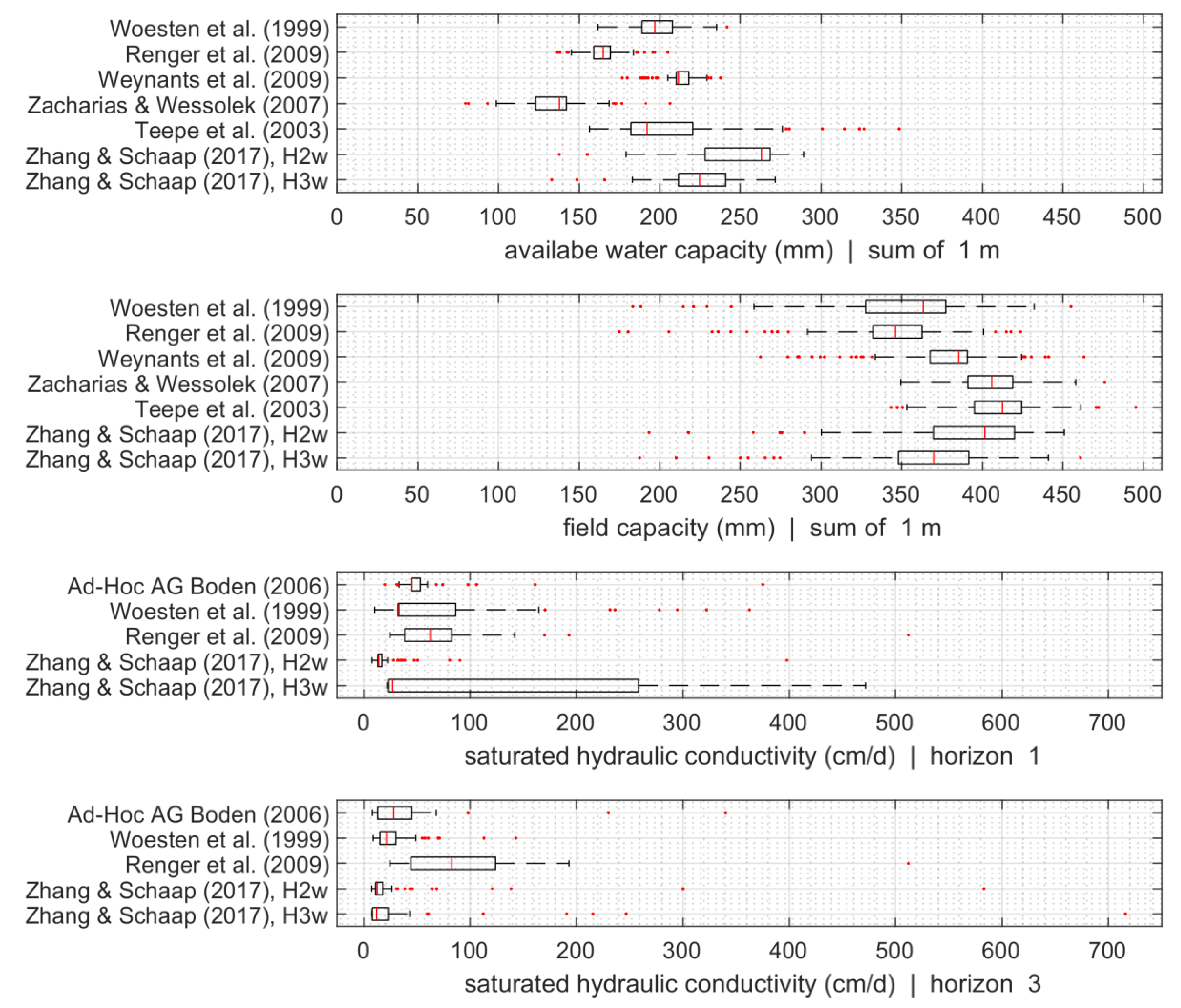
The distribution of the selected soil hydraulic properties in the Glonn catchment is displayed in Figure 2. The data contains all cells with cropland, grassland and forest land use, whereas sealed areas and water bodies are not included. AWC and FC were summarized for the uppermost meter of the soil profile. In contrast, the Ksat is presented for the top layer (horizon 1) and for the soil horizon 3, which accounts for a depth of about 75 cm. The thickness of the horizons, and consequently the depths of them, vary among the soil types. For AWC and FC, we included all PTFs, which have their own specific equation to estimate Ksat, and those that consider the parametrization of Ad-hoc-AG Boden [32] for Ksat.
The median values of the soil hydraulic properties as well as the size of the interquartile ranges show a clear dependency on the respective PTF. The range of the median values is larger for AWC than for FC, whereas the size of the interquartile ranges or the total variability is larger for FC. Accordingly, for each PTF, AWC is relatively similar within one PTF for all soil types within the catchment, most notably in the PTFs of Wösten et al. (1999) [19], Renger et al. (2009) [35], and Weynants et al. (2009) [36]. The values of AWC for the PTF of Wösten et al. (1999) [19], which is considered in the baseline scenario, range within the values of the other PTFs. The lowest AWC values were determined using the PTF of Zacharias & Wessolek (2007) [37]. The PTF with the most frequent large AWC values is the one of Zhang & Schaap (2017) [39] that does not consider bulk density as input (Rosetta H2w). The distinction in the ranges of AWC values amongst the PTFs are pronounced differently from those of FC. This indicates the variability of the available soil water storage volumes depending on the preconditions.
The range of simulated Ksat by the baseline scenario (defined according to Ad-Hoc AG Boden, 2006) [32] is within the values of the other PTFs for the considered horizons. The largest median of Ksat was defined via Renger et al. (2009) [35]. This PTF is also the only one for which the median increases from horizon 1 to horizon 3. The distinctly smaller variability of Ksat in Rosetta H2w compared to Rosetta H3w is due to the lack of consideration of the bulk density in Rosetta H2w.
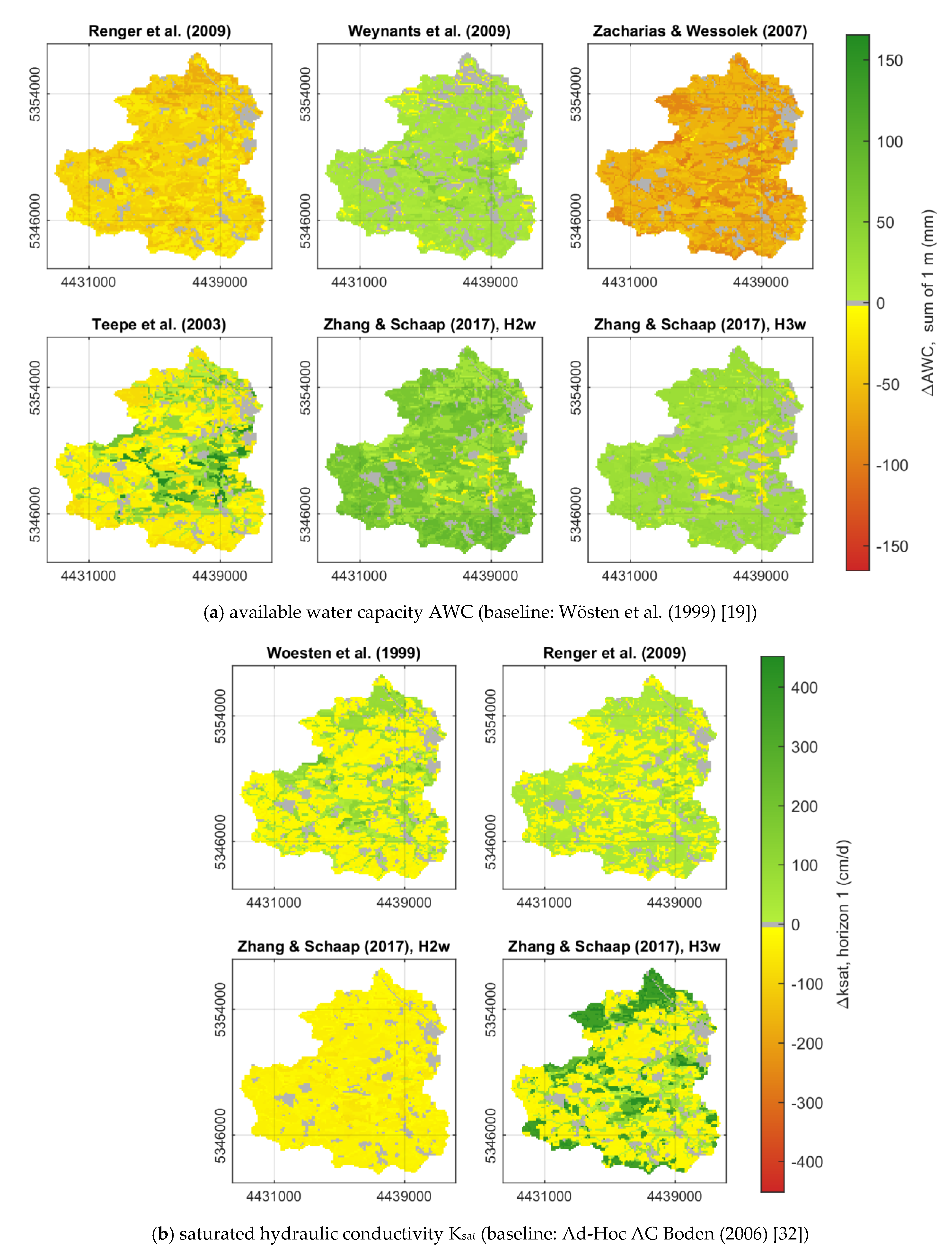
The largest spatial variation of the AWC differences (∆AWC) was found for Teepe et al. (2003) [38]. Here, the soil water storage capacities of flat areas with forest or grassland cover are increased (compared to baseline scenario), while decreased for other land uses. This observation is in accordance with the distribution displayed in Figure 2, which shows a similar median as the baseline scenario, but a distinctly larger variability. The PTF of Zacharias & Wessolek (2007) [37] results in an overall lower soil water storage with lower values in valleys and thus a contrasting behavior compared to Teepe et al. (2003) [38]. Weynants et al. (2009) [36] and both versions of Zhang & Schaap (2017) [39] show a predominantly higher soil water storage with some exceptions next to the rivers. In most cases, the areas of lower AWC in Weynants et al. (2009) [36] are not equal to those of Zhang & Schaap (2017) [39].
The shapes of the water retention curves are influenced by the input parameters of the PTFs as well as the databases used for their development (Table 4). Accordingly, the dependency of the soil water storage capacity can be related to the land use types, which affect the bulk density and organic matter content of the respective soil type. Furthermore, the variation of the soil texture class can have different effects on soil water holding capacities depending on the PTF that results in the observed non-linear shift of the soil hydraulic properties between the scenarios and the baseline scenario.
The saturated hydraulic conductivities in the topmost soil horizon of Renger et al. (2009) [35] are mostly larger than those of Ad-Hoc AG Boden (2006) [32], whereas those of Zhang & Schaap (2017), H2w [39] are lower (Figure 3b). The largest differences compared to the baseline scenario (∆Ksat) were observed in Zhang and Schaap (2017), H3w [39]. Forest sites result in much higher values of Ksat, while the increase is less distinct on grassland sites. On cropland, the Ksat values of Zhang & Schaap (2017) [39], H3w are mostly lower than those of Ad-Hoc AG Boden (2006) [32]. The differences in Wösten et al. (1999) [19] are also attributed to the land use type but less distinguished. The dependency of Ksat on the land use type is driven by the inclusion of bulk density and/or organic matter content in the PTFs.
3.2. Runoff Response
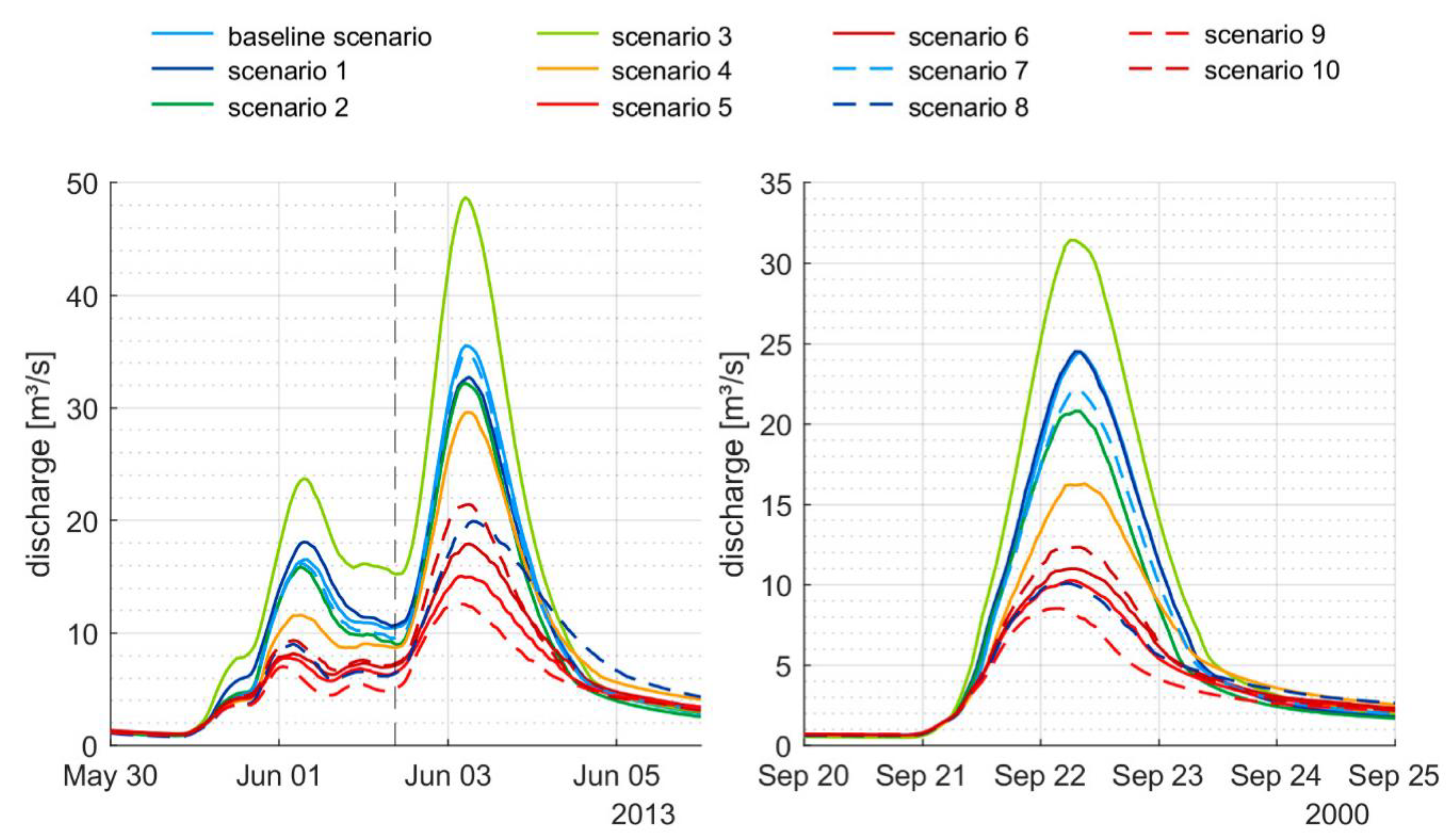
The different soil hydraulic properties of the PTFs result in a change in runoff behavior that is evident in both the total volume and the event characteristics. Figure 4 shows the hydrographs of the different scenarios (model runs) for two exemplary flood events. The quantitative evaluation of the peak and volume changes are summarized in Table 5. The double-peaked event in June 2013 was analyzed separately for the first and second wave. The range of runoff peaks of the different scenarios compared to the baseline scenario is between +43% and −65% (Table 5).
The largest runoff response occurred in scenario 3, which is based on the PTF of Zacharias & Wessolek (2007) [37], which resulted in the lowest AWC values, in comparison to other PTFs (Figure 2). The lowest runoff peaks and volumes occur in Scenarios 5 and 9, which are based on Rosetta (H2w). This PTF resulted in the largest AWC values compared to the different PTFs (Figure 2). The distinctly larger antecedent soil moisture conditions during the second peak of the flood event in June 2013 results in a different change in runoff behavior depending on the PTF. It can lead to a decrease in the percent peak change (Scenario 4), an increase in the percent peak change (Scenario 2), or even in a reversal in the direction of the peak change (Scenario 1) compared to the baseline scenario (Figure 2, Table 5). The volume changes of the calibration and validation period are small compared to those of the events. The variations indicate a different behavior in distinct discharge ranges, whose separate analysis is therefore of special interest.
For a quantitative analysis of the change in modeled runoff behavior caused by the choice of PTFs as well as the change in distinct discharge ranges, the flow duration curves at the basin outlet were compared, and four signature indices were calculated (Table 6).
As expected, Scenario 7 shows only minor deviations in catchment behavior. However, there are obvious deviations in estimating the water balance by different scenarios (%Bias_RR; e.g., underestimated up to −5.7% for scenario 4), revealing that the choice of PTF has a considerable impact on the estimated evapotranspiration. Regarding the reactivity (%Bias_Midslope), the tendency of scenarios 3, 4, and 6 is similar: showing markedly increased values (highly overestimated compared to the baseline scenario), that indicates a fast reaction of catchment to rainfall events and its direct transformation into runoff. In contrast, most scenarios exhibit an underestimation of the discharge peaks, only the scenarios 1 and 3 overestimate the peaks (positive value of %BiasFHV). Concerning the low flows (related to base flow components), we can see a contrasting model behavior for the scenarios: While the hydrological model tends to underestimate low flows for most of the scenarios (distinctly pronounced in case 3, 4, and 6), a severe underestimation of low flows results from scenario 3 (−47.2%).
3.3. Water Balance Components and Spatial Pattern Analysis
The differences in the runoff behavior amongst the scenarios can be addressed by analyzing the respective water balance and infiltration components. As displayed in Table 7, there are noticeable changes occurring in the runoff components as well as in the components influenced by the soil hydraulic properties, i.e., evaporation from the soil and change in soil water storage. The soil hydraulic properties also control the amount of matrix infiltration, which affects the infiltration excess and consequently the surface runoff.
The large runoff reactivity of scenario 3 (Figure 3) can be attributed to an increased amount of surface runoff (Table 7) which is caused by a reduction in matrix infiltration and a resulting decrease in baseflow. Compared to the baseline scenario, scenario 4 shows a slightly increased matrix infiltration and correspondingly a reduced surface runoff volume. Larger differences occur in the slower runoff components, with a significant reduction in the interflow volume and an increase in the magnitude of the baseflow. Although there is only little increase in total infiltration compared to the baseline scenario, the change in soil hydraulic properties results in a more efficient transport of water to deeper soil layers. The evaporation volumes of the scenarios 3 and 4 are the largest in comparison to other scenarios, and are about 7% higher than the baseline scenario.
The lowest runoff response of the all scenarios occurs for the scenarios 5, 6, 9, and 10. In these scenarios, surface runoff volumes are reduced in a uniform manner by about 10–13% compared to the baseline scenario. The changes in interflow and baseflow are more diverse. While the volumes are only slightly changed in scenario 5, a significant increase in interflow with a simultaneous large reduction in baseflow could be observed in scenarios 6 and 10. In contrast, in scenario 9, the interflow is reduced and the baseflow is increased, resulting in an enhanced proportion of surface runoff during the events and leading to the earlier and lower peak discharge as observed in Figure 3 compared to scenario 5. We can conclude that in both cases the use of Ksat estimated by the respective PTFs leads to a reduction in interflow and an increase in baseflow (scenarios 5 and 6 compared to 9 and 10). This behavior is more pronounced between scenarios 5 and 9 (Rosetta, H2w) than between scenarios 6 and 10 (Rosetta, H3w).
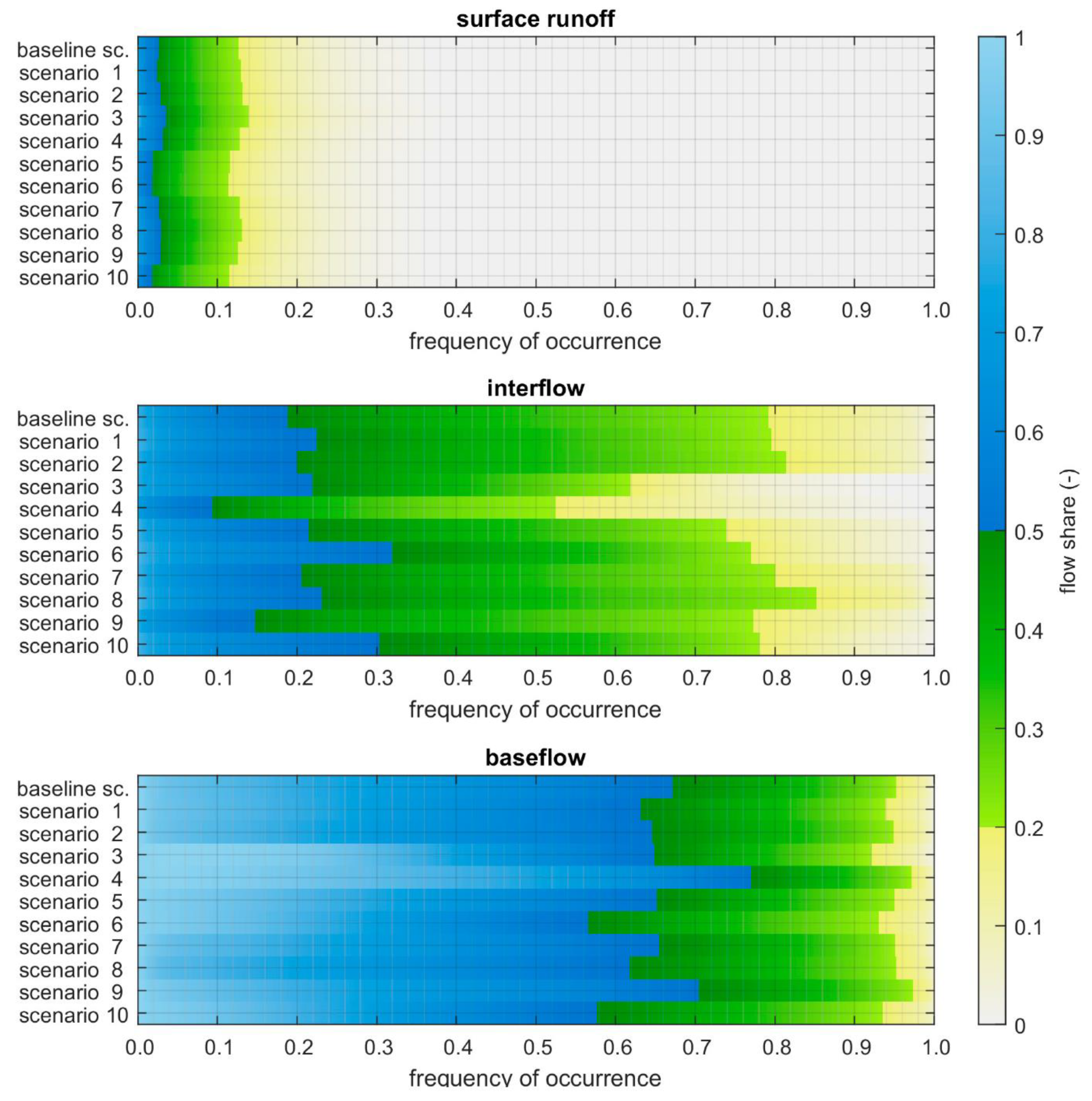
Figure 5 shows the frequency of occurrence of different flow shares for all runoff components. Blue colors indicate the dominance of the respective component (probability > 50%), green colors indicate a flow share of 20–50%, whereas yellow to grey colors indicate a probability below 20% for the respective runoff component. Scenarios 5, 6, and 10 show the shortest time periods dominated by surface runoff. While Scenario 5 shows dominance of baseflow in relatively longer time periods, Scenarios 6 and 10 remarkably indicate longer periods with interflow as dominant runoff generation process. Scenarios 4 and 9 have the shortest periods with dominant interflow but the longest with baseflow as the dominant runoff generation process.
In order to compare the spatial patterns of the evapotranspiration and runoff components simulated by 10 scenarios to the baseline scenario, we analyzed the Pearson correlation coefficient α and percentage of histogram overlap γ, considering the spatial mean of direct runoff, interflow, baseflow, and actual evapotranspiration (ETa) (Table 8).
For direct runoff, the spatial correlation of occurrence is very high but the absolute amount is different, which is indicated by a low histogram overlap. For interflow, some scenarios show both low spatial correlation and low histogram overlap, indicating that the PTF has a high impact on this runoff generation process in the model. In contrast, the baseflow pattern is similar in all scenarios. Interestingly, in all scenarios, the ETa pattern show a high correlation, however, the absolute values seem to differ considerably (relatively low values for histogram overlap).
4. Discussion
The selection of the PTF to estimate the soil hydraulic properties which are included in a hydrological model is often done without taking the runoff characteristics of the catchment into consideration. Therefore, it is of particular interest to the modeling community to have a quantitative description of the change in model behavior caused by the choice of PTF, in order to make decisions that are more informed. We hypothesized that the water balance and runoff behavior of a catchment are distinctly affected by the characteristics of the PTFs that primarily represent the water retention and hydraulic conductivity curves. Thus, we considered the soil parameterization of different PTFs in a hydrological catchment model to quantify the changes in soil hydraulic properties of the Glonn catchment as well as to analyze the resulting shifts in its water balance components and runoff characteristics.
As shown in Figure 1b, the Glonn catchment covers a wide range of different soil texture classes. It is therefore well suited for studying the influence of PTFs on soil hydraulic properties as well as the resulting runoff behavior. This high diversity allowed holding a more profound analysis of the spatial and temporal variability of different runoff characteristics depending on the choice of the respective PTF. The good representation of the runoff behavior by WaSiM-ETH suggests the general suitability of this hydrological model for the intended investigation. Moreover, the implementation of a layered soil structure made it possible to consider the underlying soil properties in detail.
The baseline scenario and the 10 other scenarios (Table 3) were chosen in such a way that the influence of modified van-Genuchten parameters or saturated hydraulic conductivities could be separately explored. Since the calibration was only performed for the baseline scenario, the differences in the runoff behavior amongst scenarios can be directly attributed to the modified soil parameters. Nevertheless, this approach cannot provide a definitive assessment of the suitability of the PTFs to represent the runoff behavior in the catchment. This evaluation would require the calibration of all scenarios using the same calibration strategy. However, due to the resulting over-imposition of the runoff behavior by the calibration parameters, the direct analysis of the particular influence of the changed soil properties would no longer be possible. Therefore, the calibration of the scenarios was not performed. Nevertheless, the parameters of the calibrated baseline scenario are within the parameter space of the other scenarios, and thus their hydrographs scatter around the measured runoff.
The considered PTFs resulted in a wide range of different shapes for the water retention and saturated hydraulic conductivity curves. The shape of the water retention curve is mainly associated with the parameters n and α which are included in the soil parameterization in WaSiM-ETH (Table 1). The parameters are related to the process of saturation and desaturation of the soil [52]. The hydraulic parameters AWC, FC, and Ksat determined for a quantitative comparison of the curves showed significant differences in their spatial distribution (Figure 2). These differences become particularly evident when comparing the individual scenarios with the baseline scenario. This issue is important because spatial variability of soil hydraulic properties is regarded as a significant factor to water distribution in the catchment [53].
The quality and quantity of the changes in the soil hydraulic properties induced by different PTFs are remarkably affected by their underlying databases, predictors, and methods used to develop the predictive equations. For example, apart from the soil texture classes, there is a significant effect on estimates of soil hydraulic properties, when both OM and BD variables and when only one of them are inputs to the equations (PTFs) [54]. Consequently, the impact of land use and geographic attributes on soil BD and OM [55] leads to a different description of the same soil in the PTFs (i.e., different input values into the equation) and this may account for the observed variation in soil hydraulic properties [11,43]. As a result, the spatial distribution of the differences that we observed between AWC and Ksat simulated by the scenarios and those of the baseline scenario could be attributed to the land use distribution as well as the proximity to watercourses (Figure 1 and Figure 3). AWC depends to a large extent on the bulk density and the silt content. Hence, PTFs that do not include BD typically result in lower AWC values in soils with lower bulk densities, such as those found in the upper soil horizons of forest soils in a study by [56,57]. They also identified the BD and soil texture as major factors explaining spatial variance in AWC for a study area in China.
The qualitative and quantitative analysis of the discharge hydrographs (Figure 4 and Table 5) as well as the respective signature indices analysis (Table 6) showed distinct differences in the runoff behavior of the catchment through investigated PTFs. The variation of the peak discharge differences between the scenarios and the baseline scenario is caused by the respective pre-event conditions, including the initial soil moisture, and consequently the available soil water storage volume, as well as infiltration capacity.
The differences in model behavior due to soil parameterizations through different PTFs were already analyzed in a study by [58] using a 1D hydrological model. They showed that even when the very same soil was considered in the entire parameterization scheme, and simulated transpiration and soil moisture were consistent with observations, yet the runoff processes or total water balance could be estimated incorrectly. Based on a multi-criteria evaluation, they found that only one of 24 investigated parameterizations resulted in a realistic behavioral model. The complexity of this evaluation is increased by focusing on a closed hydrological catchment, as it was considered in this study. Here, in comparison to above-mentioned 1D model (i.e., only one cell), adjusting the soil hydraulic properties in our catchment model by various PTFs affects the neighboring cells in the spatial domain as well.
In addition, the runoff behavior in the model is influenced by the choice of the calibration parameters. As a result, an insufficient parameterization of the soil can be at least partially compensated by an appropriate adjustment of the model calibration. However, even after calibration, a model may still represent an unrealistic water distribution across the landscape [59]. Therefore, in addition to get the right answer, for example by comparing runoff hydrographs at the catchment outlet, it is also required to analyze whether we are getting the “right answers for the right reasons” [60].
Ultimately, depending on the soil and topographic characteristics, we tracked the spatial distributions of the changes in the main hydrological processes (Table 7 and Table 8, Figure 5).
Our results led to a similar conclusion where remarkable differences amongst water balance components of the individual scenarios against the calibrated case were obtained. Furthermore, analysis of frequency of occurrence of runoff components (Figure 5) displayed a pronounced contrast amongst scenarios. This indicates that the dominance of surface runoff, interflow, and baseflow within the catchment and during time periods can be shifted depending on how the soil hydraulic properties are parameterized. In addition to temporal patterns of runoff components, we examined the spatial patterns of runoff and evapotranspiration in the catchment (Table 8). The outcome was relevant to the previous mentioned argument, where spatial patterns were also quite distinguishable amongst different scenarios. The quantified influence of various PTFs on temporal and spatial patterns of water budget components provided the same evidence to the fact that spatial variability in soil hydraulic characteristics and model errors initiated from application of different PTF cases, may introduce their own uncertainty to model simulation. This is consistent with what has been found by [61]. They compared the performance of two different soil hydraulic parameterization techniques in terms of outputs of catchment water balance simulated by the model HydroGeoSphere, and underlined the potential flaws of choosing different parameterizations in spatially distributed modeling.
Finally, it may be concluded that the information contained in streamflow data is not sufficient to derive physically reasonable soil parameter values only via calibration. This indicates that the resulted uncertainty most likely comes from different descriptions of soil water characteristics (i.e., PTF cases). On this account, deriving the “spatial distribution of variability” from different scenarios, our methodology revealed that choosing a specific PTF may significantly influence the spatial distribution of soil hydraulic properties (e.g., Ksat and AWC) and also the way water is being distributed across the landscape prior to the catchment outlet. As a result, owing to the fact that the spatial variability of Ksat and AWC affects the temporal response of the catchment to precipitation and runoff concentration, one can consider that selection of a particular PTF makes evident changes in the distribution among groundwater infiltration, runoff and evapotranspiration in the catchment [53,62].
It is important to highlight the fact that most of the PTFs yet show limitations considering the effects of soil inhomogeneity due to structure or macropores, and widely available soil datasets (e.g., FAO Harmonized World Soil Database) may fail to reflect actual field conditions. This warrants further evaluation of PTFs using extensive observed data and particular inclusion the effects of soil structure and macropores [39,63]. Moreover, since soil hydrological parameters vary significantly even within a small area, most of the PTFs are usually applicable with acceptable accuracy only in the regions where those functions were developed [64]. This study showed that the uncertainly forced by selection of PTFs are mainly represented in the spatial distribution of runoff components which are not distinctly addressed by hydrological model calibration against observed discharge time series at the catchment outlet. This recommends that emphasis should be made to soil parameterization oriented towards a “plausible hydrological behavior in terms of spatial patterns of runoff components” during catchment modeling.
According to our knowledge, no comprehensive work was dedicated to carefully analyze the impact of different PTF selection on spatial distribution of internal hydrological processes in the catchment, which underlines the novelty of this research. Indeed, at this stage of understanding, the question of “which PTFs are performing the best?” still remains to be addressed. Since answering this question is beyond the topic of this paper, we therefore believe that future research is clearly required to quantify and qualify the spatial difference in distribution of internal hydrological processes introduced by various PTFs. In other words, application of PTFs in hydrological models without evaluating the spatial patterns of soil moisture, evapotranspiration, and runoff processes produced by different PTFs may ultimately lead to implausible results and possibly to incorrect decisions in water management. This entails investigation of additional information, which usually has to be elaborately collected, for instance, by mapping the dominant runoff generation processes in the area, or retrieving the spatial patterns of evapotranspiration and soil moisture using remote sensing methods, and evaluation at a scale commensurate with hydrological model [51,65].
5. Conclusions
The knowledge of soil hydraulic properties and land use effects on these properties are important for efficient soil and water management. Hence, the motivation for this study was to examine a methodology to quantify the effect of modeler’s choice of PTF on van Genuchten parameters, and accordingly, analyze the sensitivity of simulated hydrological processes to the spatial variability in soil hydraulic characteristics associated with different PTFs. Our results cast a new light on the way that PTFs are routinely being opted for parameterization of hydrologic modeling (i.e., parameters of van Genuchten). It was revealed that elements of the water balance are highly sensitive to the spatial structure of soil hydraulic properties, and a wide range of different hydrological model behavior can be created just by the option of PTFs. Despite the different proportions of various runoff components produced by a variety of PTFs, this might still result in an acceptable representation of the discharge hydrograph. As a result, model calibration exclusively at catchment outlet may lead to implausible results and possibly to incorrect decisions. Since the distribution of water in the hydrologic system differs greatly amongst PTF cases, we recommend aligning the soil parameterization more towards mapping a plausible hydrological behavior. Nevertheless, to this end, additional information is required, which usually has to be intricately clustered together, for example, by mapping the dominant runoff processes in the hydrologic system; or deriving the soil moisture and evapotranspiration patterns by remote sensing methods.
Author Contributions
Conceptualization, H.M. and M.C.C.; Methodology, S.T., H.M. and M.C.C.; Software, S.T. and M.C.C.; Validation, H.M., S.T. and M.C.C.; Resources, M.C.C.; Data curation, S.T. and M.C.C.; Writing—original draft preparation, H.M.; Writing—review and editing, H.M., S.T. and M.C.C.; Visualization, S.T.; Supervision, M.C.C.; Project administration, M.C.C.; Funding acquisition, M.C.C. All authors have read and agreed to the published version of the manuscript.
Funding
This work has been funded by the Deutsche Forschungsgemeinschaft (DFG, German Research Foundation)—426111700.
Institutional Review Board Statement
Not applicable.
Informed Consent Statement
Not applicable.
Data Availability Statement
The data presented in this study are available on request from the corresponding author.
Conflicts of Interest
The authors declare no conflict of interest.
References
- Gupta, H.V.; Beven, K.J.; Wagener, T. Model Calibration and Uncertainty Estimation. In Encyclopedia of Hydrological Sciences; John Wiley & Sons, Ltd.: Hoboken, NJ, USA, 2006. [Google Scholar] [CrossRef]
- Elsenbeer, H. Hydrologic Flowpaths in Tropical Rainforest Soilscapes—A Review. Hydrol. Process. 2001, 15, 1751–1759. [Google Scholar] [CrossRef]
- Montzka, C.; Herbst, M.; Weihermüller, L.; Verhoef, A.; Vereecken, H. A Global Data Set of Soil Hydraulic Properties and Sub-Grid Variability of Soil Water Retention and Hydraulic Conductivity Curves. Earth Syst. Sci. Data 2017, 9, 529–543. [Google Scholar] [CrossRef] [Green Version]
- Arnold, J.G.; Muttiah, R.S.; Srinivasan, R.; Allen, P.M. Regional Estimation of Base Flow and Groundwater Recharge in the Upper Mississippi River Basin. J. Hydrol. 2000, 227, 21–40. [Google Scholar] [CrossRef]
- Rieger, W.; Disse, M. Physikalisch Basierter Modellansatz Zur Beurteilung Der Wirksamkeit Einzelner Und Kombinierter Dezentraler Hochwasserschutzmaßnahmen. Hydrol. Wasserbewirtsch. 2013, 57, 14–25. [Google Scholar] [CrossRef]
- Richards, L.A. Capillary Conduction of Liquids through Porous Mediums. Physics 1931, 1, 318–333. [Google Scholar] [CrossRef]
- Ebel, B.A.; Loague, K. Physics-Based Hydrologic-Response Simulation: Seeing through the Fog of Equifinality. Hydrol. Process. Int. J. 2006, 20, 2887–2900. [Google Scholar] [CrossRef]
- Qu, Y.; Duffy, C.J. A Semidiscrete Finite Volume Formulation for Multiprocess Watershed Simulation. Water Resour. Res. 2007, 43, W08419. [Google Scholar] [CrossRef]
- Ivanov, V.Y.; Bras, R.L.; Vivoni, E.R. Vegetation-Hydrology Dynamics in Complex Terrain of Semiarid Areas: 1. A Mechanistic Approach to Modeling Dynamic Feedbacks. Water Resour. Res. 2008, 44, W03429. [Google Scholar] [CrossRef] [Green Version]
- Te Chow, V. Applied Hydrology; Tata McGraw-Hill Education: Pennsylvania Plaza, NY, USA, 2010. [Google Scholar]
- Wösten, J.; Pachepsky, Y.A.; Rawls, W. Pedotransfer Functions: Bridging the Gap between Available Basic Soil Data and Missing Soil Hydraulic Characteristics. J. Hydrol. 2001, 251, 123–150. [Google Scholar] [CrossRef]
- Bogena, H.; Herbst, M.; Huisman, J.; Rosenbaum, U.; Weuthen, A.; Vereecken, H. Potential of Wireless Sensor Networks for Measuring Soil Water Content Variability. Vadose Zone J. 2010, 9, 1002–1013. [Google Scholar] [CrossRef] [Green Version]
- Brooks, R.H.; Corey, A.T. Properties of Porous Media Affecting Fluid Flow. J. Irrig. Drain. Div. 1966, 92, 61–88. [Google Scholar] [CrossRef]
- Mualem, Y. A New Model for Predicting the Hydraulic Conductivity of Unsaturated Porous Media. Water Resour. Res. 1976, 12, 513–522. [Google Scholar] [CrossRef] [Green Version]
- Van Genuchten, M.T. A Closed-Form Equation for Predicting the Hydraulic Conductivity of Unsaturated Soils 1. Soil Sci. Soc. Am. J. 1980, 44, 892–898. [Google Scholar] [CrossRef] [Green Version]
- Aubertin, G.M.; Patric, J.H. Water Quality after Clearcutting a Small Watershed in West Virginia. J. Environ. Qual. 1974, 3, 243–249. [Google Scholar] [CrossRef] [Green Version]
- Vereecken, H.; Weynants, M.; Javaux, M.; Pachepsky, Y.; Schaap, M.; Van Genuchten, M.T. Using Pedotransfer Functions to Estimate the van Genuchten–Mualem Soil Hydraulic Properties: A Review. Vadose Zone J. 2010, 9, 795–820. [Google Scholar] [CrossRef]
- Bouma, J. Using Soil Survey Data for Quantitative Land Evaluation. In Advances in Soil Science; Springer: Berlin/Heidelberg, Germany, 1989; pp. 177–213. [Google Scholar]
- Wösten, J.; Lilly, A.; Nemes, A.; Le Bas, C. Development and Use of a Database of Hydraulic Properties of European Soils. Geoderma 1999, 90, 169–185. [Google Scholar] [CrossRef]
- Pachepsky, Y.; Rawls, W.J. Development of Pedotransfer Functions in Soil Hydrology; Elsevier: Amsterdam, The Netherlands, 2004; Volume 30, ISBN 978-0-444-51705-0. [Google Scholar]
- Patil, N.G.; Singh, S.K. Pedotransfer Functions for Estimating Soil Hydraulic Properties: A Review. Pedosphere 2016, 26, 417–430. [Google Scholar] [CrossRef]
- Schaap, M.G.; Leij, F.J. Using Neural Networks to Predict Soil Water Retention and Soil Hydraulic Conductivity. Soil Tillage Res. 1998, 47, 37–42. [Google Scholar] [CrossRef]
- Schaap, M.G.; Bouten, W. Modeling Water Retention Curves of Sandy Soils Using Neural Networks. Water Resour. Res. 1996, 32, 3033–3040. [Google Scholar] [CrossRef]
- Grayson, R.B.; Blöschl, G.; Western, A.W.; McMahon, T.A. Advances in the Use of Observed Spatial Patterns of Catchment Hydrological Response. Adv. Water Res. 2002, 25, 1313–1334. [Google Scholar] [CrossRef]
- Beven, K. Towards an Alternative Blueprint for a Physically Based Digitally Simulated Hydrologic Response Modelling System. Hydrol. Process. 2002, 16, 189–206. [Google Scholar] [CrossRef] [Green Version]
- Vereecken, H.; Diels, J.; Van Orshoven, J.; Feyen, J.; Bouma, J. Functional Evaluation of Pedotransfer Functions for the Estimation of Soil Hydraulic Properties. Soil Sci. Soc. Am. J. 1992, 56, 1371–1378. [Google Scholar] [CrossRef]
- Vereecken, H.; Maes, J.; Feyen, J.; Darius, P. Estimating the Soil Moisture Retention Characteristic from Texture, Bulk Density, and Carbon Content. Soil Sci. 1989, 148, 389–403. [Google Scholar] [CrossRef]
- Vereecken, H.; Maes, J.; Feyen, J. Estimating Unsaturated Hydraulic Conductivity from Easily Measured Soil Properties. Soil Sci. 1990, 149, 1–12. [Google Scholar] [CrossRef]
- Chirico, G.; Medina, H.; Romano, N. Functional Evaluation of PTF Prediction Uncertainty: An Application at Hillslope Scale. Geoderma 2010, 155, 193–202. [Google Scholar] [CrossRef]
- Seibert, J. Regionalisation of Parameters for a Conceptual Rainfall-Runoff Model. Agric. For. Meteorol. 1999, 98, 279–293. [Google Scholar] [CrossRef]
- Eckelmann, W.; Sponagel, H.; Grottenthaler, W.; Hartmann, K.-J.; Hartwich, R.; Janetzko, P.; Joisten, H.; Kühn, D.; Sabel, K.-J.; Traidl, R. Bayrisches Landesamt für Wasserwirtschaft: Fließgewässerlandschaften in Bayern; BAYERN|DIREKT: München, Germany, 2002. [Google Scholar]
- Ad-hoc-AG Boden Bodenkundliche Kartieranleitung, 5th ed.; Schweizerbart Science Publishers: Stuttgart, Germany, 2006; ISBN 978-3-510-95920-4.
- Schulla, J. Model Description WaSiM (Water Balance Simulation Model); Hydrology Software Consulting: Zürich, Switzerland, 2019; p. 379. [Google Scholar]
- Moriasi, D.N.; Arnold, J.G.; Van Liew, M.W.; Bingner, R.L.; Harmel, R.D.; Veith, T.L. Model Evaluation Guidelines for Systematic Quantification of Accuracy in Watershed Simulations. Trans. ASABE 2007, 50, 885–900. [Google Scholar] [CrossRef]
- Renger, M.; Bohne, K.; Facklam, M.; Harrach, T.; Riek, W.; Schäfer, W.; Wessolek, G.; Zacharias, S. Ergebnisse Und Vorschläge Der DBG-Arbeitsgruppe “Kennwerte Des Bodengefüges” Zur Schätzung Bodenphysikalischer Kennwerte. Acad. Accel. World’s Res. 2008, 40, 4–51. [Google Scholar]
- Weynants, M.; Vereecken, H.; Javaux, M. Revisiting Vereecken Pedotransfer Functions: Introducing a Closed-Form Hydraulic Model. Vadose Zone J. 2009, 8, 86–95. [Google Scholar] [CrossRef] [Green Version]
- Zacharias, S.; Wessolek, G. Excluding Organic Matter Content from Pedotransfer Predictors of Soil Water Retention. Soil Sci. Soc. Am. J. 2007, 71, 43–50. [Google Scholar] [CrossRef]
- Teepe, R.; Dilling, H.; Beese, F. Estimating Water Retention Curves of Forest Soils from Soil Texture and Bulk Density. J. Plant Nutr. Soil Sci. 2003, 166, 111–119. [Google Scholar] [CrossRef]
- Zhang, Y.; Schaap, M.G. Weighted Recalibration of the Rosetta Pedotransfer Model with Improved Estimates of Hydraulic Parameter Distributions and Summary Statistics (Rosetta3). J. Hydrol. 2017, 547, 39–53. [Google Scholar] [CrossRef] [Green Version]
- Tóth, B.; Weynants, M.; Pásztor, L.; Hengl, T. 3D Soil Hydraulic Database of Europe at 250 m Resolution. Hydrol. Process. 2017, 31, 2662–2666. [Google Scholar] [CrossRef] [Green Version]
- Rajkai, K.; Kabos, S.; Van Genuchten, M.T. Estimating the Water Retention Curve from Soil Properties: Comparison of Linear, Nonlinear and Concomitant Variable Methods. Soil Tillage Res. 2004, 79, 145–152. [Google Scholar] [CrossRef]
- Wessolek, G.; Duijnisveld, W.; Trinks, S. Hydro-Pedotransfer Functions (HPTFs) for Predicting Annual Percolation Rate on a Regional Scale. J. Hydrol. 2008, 356, 17–27. [Google Scholar] [CrossRef]
- Nemes, A.; Schaap, M.; Leij, F.; Wösten, J. Description of the Unsaturated Soil Hydraulic Database UNSODA Version 2.0. J. Hydrol. 2001, 251, 151–162. [Google Scholar] [CrossRef]
- Tempel, P.; Batjes, N.; Van Engelen, V. IGBP-DIS Soil Data Set for Pedotransfer Function Development. ISRIC 1996, 447365. [Google Scholar]
- Schaap, M.G.; Leij, F.J.; Van Genuchten, M.T. Rosetta: A Computer Program for Estimating Soil Hydraulic Parameters with Hierarchical Pedotransfer Functions. J. Hydrol. 2001, 251, 163–176. [Google Scholar] [CrossRef]
- Vogel, R.M.; Fennessey, N.M. Flow-Duration Curves. I: New Interpretation and Confidence Intervals. J. Water Res. Plan. Manag. 1994, 120, 485–504. [Google Scholar] [CrossRef]
- Smakhtin, V.U. Low Flow Hydrology: A Review. J. Hydrol. 2001, 240, 147–186. [Google Scholar] [CrossRef]
- Yilmaz, K.K.; Gupta, H.V.; Wagener, T. A Process-Based Diagnostic Approach to Model Evaluation: Application to the NWS Distributed Hydrologic Model. Water Resour. Res. 2008, 44, W09417. [Google Scholar] [CrossRef] [Green Version]
- Casper, M.C.; Grigoryan, G.; Gronz, O.; Gutjahr, O.; Heinemann, G.; Ley, R.; Rock, A. Analysis of Projected Hydrological Behavior of Catchments Based on Signature Indices. Hydrol. Earth Syst. Sci. 2012, 16, 409–421. [Google Scholar] [CrossRef] [Green Version]
- Swain, M.J.; Ballard, D.H. Color Indexing. Int. J. Comput. Vis. 1991, 7, 11–32. [Google Scholar] [CrossRef]
- Demirel, M.C.; Mai, J.; Mendiguren, G.; Koch, J.; Samaniego, L.; Stisen, S. Combining Satellite Data and Appropriate Objective Functions for Improved Spatial Pattern Performance of a Distributed Hydrologic Model. Hydrol. Earth Syst. Sci. 2018, 22, 1299–1315. [Google Scholar] [CrossRef] [Green Version]
- Wang, J.-P.; Hu, N.; François, B.; Lambert, P. Estimating Water Retention Curves and Strength Properties of Unsaturated Sandy Soils from Basic Soil Gradation Parameters. Water Resour. Res. 2017, 53, 6069–6088. [Google Scholar] [CrossRef]
- Zheng, J.; Shao, M.; Zhang, X. Spatial Variation of Surface Soil’s Bulk Density and Saturated Hydraulic Conductivity on Slope in Loess Region. J. Soil Water Conserv. 2004, 18, 53–56. [Google Scholar] [CrossRef]
- Nemes, A.; Rawls, W.J.; Pachepsky, Y.A. Influence of Organic Matter on the Estimation of Saturated Hydraulic Conductivity. Soil Sci. Soc. Am. J. 2005, 69, 1330–1337. [Google Scholar] [CrossRef]
- Azuka, C.; Igué, A. Surface Runoff as Influenced by Slope Position and Land Use in the Koupendri Catchment of Northwest Benin: Field Observation and Model Validation. Hydrol. Sci. J. 2020, 65, 995–1004. [Google Scholar] [CrossRef]
- Dobarco, M.R.; Bourennane, H.; Arrouays, D.; Saby, N.P.; Cousin, I.; Martin, M.P. Uncertainty Assessment of GlobalSoilMap Soil Available Water Capacity Products: A French Case Study. Geoderma 2019, 344, 14–30. [Google Scholar] [CrossRef]
- Li, X.; Shao, M.; Zhao, C.; Jia, X. Spatial Variability of Soil Water Content and Related Factors across the Hexi Corridor of China. J. Arid Land 2019, 11, 123–134. [Google Scholar] [CrossRef] [Green Version]
- Casper, M.C.; Mohajerani, H.; Hassler, S.K.; Herdel, T.; Blume, T. Finding Behavioral Parameterization for a 1-D Water Balance Model by Multi-Criteria Evaluation. J. Hydrol. Hydromech. 2019, 67, 213–224. [Google Scholar] [CrossRef] [Green Version]
- Rajib, A.; Evenson, G.R.; Golden, H.E.; Lane, C.R. Hydrologic Model Predictability Improves with Spatially Explicit Calibration Using Remotely Sensed Evapotranspiration and Biophysical Parameters. J. Hydrol. 2018, 567, 668–683. [Google Scholar] [CrossRef] [PubMed]
- Kirchner, J.W. Getting the Right Answers for the Right Reasons: Linking Measurements, Analyses, and Models to Advance the Science of Hydrology. Water Resour. Res. 2006, 42. [Google Scholar] [CrossRef]
- Nasta, P.; Boaga, J.; Deiana, R.; Cassiani, G.; Romano, N. Comparing ERT-and Scaling-Based Approaches to Parameterize Soil Hydraulic Properties for Spatially Distributed Model Applications. Adv. Water Res. 2019, 126, 155–167. [Google Scholar] [CrossRef]
- Herbst, M.; Diekkrüger, B. The Influence of the Spatial Structure of Soil Properties on Water Balance Modeling in a Microscale Catchment. Phys. Chem. Earth Parts A/B/C 2002, 27, 701–710. [Google Scholar] [CrossRef]
- Bayabil, H.K.; Dile, Y.T.; Tebebu, T.Y.; Engda, T.A.; Steenhuis, T.S. Evaluating Infiltration Models and Pedotransfer Functions: Implications for Hydrologic Modeling. Geoderma 2019, 338, 159–169. [Google Scholar] [CrossRef]
- Li, Y.; Chen, D.; White, R.E.; Zhu, A.; Zhang, J. Estimating Soil Hydraulic Properties of Fengqiu County Soils in the North China Plain Using Pedo-Transfer Functions. Geoderma 2007, 138, 261–271. [Google Scholar] [CrossRef]
- Casper, M.C.; Vohland, M. Validation of a Large Scale Hydrological Model with Data Fields Retrieved from Reflective and Thermal Optical Remote Sensing Data—A Case Study for the Upper Rhine Valley. Phys. Chem. Earth Parts A/B/C 2008, 33, 1061–1067. [Google Scholar] [CrossRef]
Figure 1.
Topography (a), soil characteristics (b), and land use (c) of the Glonn catchment.

Figure 2.
Distribution of the soil hydraulic properties AWC, FC, and Ksat for the land use types cropland, grassland and Forest in the Glonn catchment.
Figure 2.
Distribution of the soil hydraulic properties AWC, FC, and Ksat for the land use types cropland, grassland and Forest in the Glonn catchment.

Figure 3.
Spatial distribution of differences in soil hydraulic properties (∆AWC, ∆Ksat). AWC is calculated for the first meter of the soil profile and the Ksat at the uppermost horizon of the soil profiles.
Figure 3.
Spatial distribution of differences in soil hydraulic properties (∆AWC, ∆Ksat). AWC is calculated for the first meter of the soil profile and the Ksat at the uppermost horizon of the soil profiles.

Figure 4.
Hydrographs of the baseline scenario and the 10 scenario runs for two exemplary events (scenario description: Table 3).
Figure 4.
Hydrographs of the baseline scenario and the 10 scenario runs for two exemplary events (scenario description: Table 3).

Figure 5.
Frequency of occurrence of flow shares for all runoff components (scenario description: Table 3).
Figure 5.
Frequency of occurrence of flow shares for all runoff components (scenario description: Table 3).


Table 1.
Mandatory parameters to describe a soil horizon in the WaSiM control file.
| Parameter | Description |
|---|---|
| Horizon | ID for each soil horizon; one value per horizon. |
| Layer | Number of numerical layers for each horizon. |
| Thickness | Thickness of each single numerical layer in this horizon in m; one value per horizon. |
| Ksat | Saturated hydraulic conductivity in m/s; one value per soil horizon. |
| Θsat | Saturated water content (fillable porosity in 1/1); one value per soil horizon. |
| Θres | Residual water content (in 1/1, water content which cannot be extracted by transpiration, only by evaporation); one value per soil horizon. |
| α | van Genuchten Parameter α; one value per soil horizon. |
| n | van Genuchten Parameter n; one value per soil horizon. |
| Krecession | Ksat recession with depth: factor of recession per meter (only applied for the uppermost 2 m of the soil); one value per horizon. |
Table 2.
Goodness of fit criteria and shares of water balance components for the calibration and validation period.
Table 2.
Goodness of fit criteria and shares of water balance components for the calibration and validation period.
| Parameter | Calibration | Validation |
|---|---|---|
| Time period | 1 November 1995–31 October 2004 | 1 November 2004–31 October 2013 |
| NSE | 0.74 | 0.65 |
| NSElog | 0.61 | 0.67 |
| PBIAS | 13.2 | −1.9 |
| Volume share of | ||
| Baseflow | 0.16 | 0.14 |
| Interflow | 0.14 | 0.14 |
| Surface runoff | 0.04 | 0.05 |
| Evapotranspiration | 0.68 | 0.67 |
Table 3.
Scenario definition: combinations of PTFs to determine the van Genuchten parameters (θsat, θres, α, n) and the saturated hydraulic conductivity (Ksat).
Table 3.
Scenario definition: combinations of PTFs to determine the van Genuchten parameters (θsat, θres, α, n) and the saturated hydraulic conductivity (Ksat).
| Scenario | Van Genuchten Parameter | Saturated Hydraulic Conductivity |
|---|---|---|
| Baseline | Wösten et al. (1999) [19] | Ad-Hoc AG Boden (2006) [32] |
| 1 | Renger et al. (2009) [35] | Ad-Hoc AG Boden (2006) [32] |
| 2 | Weynants et al. (2009) [36] | Ad-Hoc AG Boden (2006) [32] |
| 3 | Zacharias & Wessolek (2007) [37] | Ad-Hoc AG Boden (2006) [32] |
| 4 | Teepe et al. (2003) [38] | Ad-Hoc AG Boden (2006) [32] |
| 5 | Zhang & Schaap (2017): Rosetta H2w [39] | Ad-Hoc AG Boden (2006) [32] |
| 6 | Zhang & Schaap (2017): Rosetta H3w [39] | Ad-Hoc AG Boden (2006) [32] |
| 7 | Wösten et al. (1999) [19] | Wösten et al. (1999) [19] |
| 8 | Renger et al. (2009) [35] | Renger et al. (2009) [35] |
| 9 | Zhang & Schaap (2017): Rosetta H2w [39] | Zhang & Schaap (2017): Rosetta H2w [39] |
| 10 | Zhang & Schaap (2017): Rosetta H3w [39] | Zhang & Schaap (2017): Rosetta H3w [39] |
Table 4.
Overview of the selected PTFs including their main characteristics.
| PTF | Method | Database | Sample Size | Predictors |
|---|---|---|---|---|
| Wösten et al. (1999) [19] | Regression analysis | HYPRES [19] | 5521 | Clay, Silt, OM, BD, topsoil/subsoil |
| Renger et al. (2009) [35] | Regression analysis | various sources | unknown | Sand, Silt, Clay |
| Weynants et al. (2009) [36] | Regression analysis | Vereecken et al., 1989 [27] | 166 | Sand, Silt, Clay, BD, OM |
| Zacharias and Wessolek (2007) [37] | Regression analysis | IGBP-DIS soil data (Tempel et al., 1996) [44]; UNSODA (Nemes et al., 2001) [43] | 676 | Sand, Silt, Clay, BD |
| Teepe et al. (2003) [38] | Regression analysis | Teepe et al. (2003) [38] | 1850 | Lookup table: Sand, Silt, Clay, BD |
| Zhang & Schaap (2017), Rosetta H2w [39] | Single Artificial Neural Network | Schaap et al. (2001) [45] | 2134 for WRC, 1306 for Ksat | Sand, Silt, Clay |
| Zhang & Schaap (2017), Rosetta H3w [39] | Single Artificial Neural Network | Schaap et al. (2001) [45] | 2134 for WRC, 1306 for Ksat | Sand, Silt, Clay, BD |
Clay: percentage of clay, Silt: percentage of silt, OM: percentage of organic matter, BD: bulk density.
Table 5.
Peak changes (%) and volume changes (%) of the selected events in Figure 4 and the calibration and validation periods the event in June 2013 is evaluated separately for both peaks.
Table 5.
Peak changes (%) and volume changes (%) of the selected events in Figure 4 and the calibration and validation periods the event in June 2013 is evaluated separately for both peaks.
| Scenario | Peak Change (%) | Volume Change (%) | ||||||
|---|---|---|---|---|---|---|---|---|
| 06/2013 (1) | 06/2013 (2) | 09/2000 | 06/2013 (1) | 06/2013 (2) | 09/2000 | calib. | valid. | |
| 1 | 9.4 | −7.9 | 0.0 | 10.0 | −4.6 | 1.0 | −4.7 | −0.5 |
| 2 | −3.8 | −9.4 | −15.1 | −5.4 | −11.1 | −13.0 | −5.2 | −4.5 |
| 3 | 43.4 | 37.0 | 28.3 | 44.1 | 29.2 | 26.8 | −6.7 | −4.7 |
| 4 | −29.8 | −16.7 | −33.6 | −20.7 | −8.0 | −18.9 | −5.7 | −4.6 |
| 5 | −52.9 | −57.6 | −58.0 | −39.9 | −42.6 | −41.1 | −0.6 | −0.7 |
| 6 | −50.5 | −49.5 | −55.1 | −36.2 | −34.6 | −36.9 | −0.9 | −0.6 |
| 7 | −2.2 | −1.9 | −9.5 | −3.6 | −2.7 | −6.6 | 0.0 | 0.4 |
| 8 | −45.3 | −43.9 | −58.8 | −39.5 | −21.7 | −39.3 | −2.4 | 0.3 |
| 9 | −57.4 | −64.6 | −65.2 | −49.8 | −50.1 | −50.4 | −0.6 | −0.8 |
| 10 | −43.3 | −39.7 | −49.6 | −32.3 | −30.4 | −34.3 | −1.9 | −1.6 |
Table 6.
Signature indices of the 10 scenarios compared to the baseline scenario; evaluation period: 1 November 1995–31 October 2013.
Table 6.
Signature indices of the 10 scenarios compared to the baseline scenario; evaluation period: 1 November 1995–31 October 2013.
| Scenario | %BiasRR | %BiasMidslope | %BiasFHV | %BiasFLV |
|---|---|---|---|---|
| 1 | −2.6 | 7.5 | 10.1 | −16.8 |
| 2 | −4.8 | 1.0 | −3.9 | −11.2 |
| 3 | −5.7 | 87.5 | 43.5 | −47.2 |
| 4 | −5.1 | 43.3 | −11.8 | −25.4 |
| 5 | −0.6 | 20.2 | −24.6 | −11.1 |
| 6 | −0.7 | 38.1 | −20.8 | −25.7 |
| 7 | 0.2 | 1.0 | −2.5 | −0.3 |
| 8 | −1.0 | −0.1 | −23.5 | 6.1 |
| 9 | −0.7 | −3.6 | −34.7 | 14.1 |
| 10 | −1.7 | 27.1 | −18.0 | −21.3 |
Table 7.
Mean annual amount of the water balance and infiltration components for the baseline scenario and the 10 scenarios.
Table 7.
Mean annual amount of the water balance and infiltration components for the baseline scenario and the 10 scenarios.
| Water Balance Components (mm/a) | Infiltration Components (mm/a) | ||||||||||||||
|---|---|---|---|---|---|---|---|---|---|---|---|---|---|---|---|
| Surface Runoff | Interflow | Base Flow | Transpiration | Evaporation | Snow Evaporation | Interception Evaporation | Change in Soil Storage | Change in Snow Storage | Infiltration Excess | Macropore infiltration | Matrix Infiltration | Interception Evaporation | Snow Evaporation | ||
| Baseline | 39 | 117 | 121 | 99 | 302 | 14 | 163 | 4 | 0 | 39 | 19 | 625 | 163 | 14 | |
| Scenario | 1 | 42 | 121 | 108 | 98 | 303 | 14 | 163 | 10 | 0 | 42 | 19 | 622 | 163 | 14 |
| 2 | 41 | 113 | 110 | 99 | 316 | 14 | 163 | 4 | 0 | 41 | 19 | 624 | 163 | 14 | |
| 3 | 50 | 117 | 95 | 99 | 323 | 14 | 163 | 0 | 0 | 50 | 18 | 615 | 163 | 14 | |
| 4 | 37 | 89 | 136 | 99 | 322 | 14 | 163 | 0 | 0 | 37 | 19 | 627 | 163 | 14 | |
| 5 | 34 | 120 | 122 | 97 | 310 | 14 | 163 | 0 | 0 | 34 | 19 | 630 | 163 | 14 | |
| 6 | 34 | 135 | 106 | 97 | 310 | 14 | 163 | 0 | 0 | 34 | 19 | 630 | 163 | 14 | |
| 7 | 39 | 121 | 119 | 99 | 302 | 14 | 163 | 4 | 0 | 39 | 19 | 625 | 163 | 14 | |
| 8 | 36 | 123 | 117 | 99 | 299 | 14 | 163 | 10 | 0 | 36 | 19 | 628 | 163 | 14 | |
| 9 | 35 | 107 | 133 | 97 | 309 | 14 | 163 | 1 | 0 | 35 | 19 | 629 | 163 | 14 | |
| 10 | 35 | 133 | 108 | 97 | 311 | 14 | 163 | 0 | 0 | 35 | 19 | 629 | 163 | 14 | |
Table 8.
Spatial correlation (correl) and histogram overlap (histo) of the 10 scenarios compared to the baseline scenario, for spatial mean of direct runoff, Interflow, baseflow, and ETa.
Table 8.
Spatial correlation (correl) and histogram overlap (histo) of the 10 scenarios compared to the baseline scenario, for spatial mean of direct runoff, Interflow, baseflow, and ETa.
| Scenario | Correl | Histo | Correl | Histo | Correl | Histo | Correl | Histo |
|---|---|---|---|---|---|---|---|---|
| Direct Runoff | Interflow | Baseflow | ETa | |||||
| 1 | 0.997 | 0.804 | 0.942 | 0.893 | 0.996 | 0.985 | 0.997 | 0.819 |
| 2 | 0.999 | 0.697 | 0.975 | 0.892 | 0.998 | 0.976 | 0.998 | 0.727 |
| 3 | 0.992 | 0.423 | 0.782 | 0.769 | 0.978 | 0.970 | 0.988 | 0.349 |
| 4 | 0.997 | 0.786 | 0.500 | 0.381 | 0.976 | 0.987 | 0.997 | 0.744 |
| 5 | 0.997 | 0.653 | 0.835 | 0.829 | 0.990 | 0.966 | 0.996 | 0.652 |
| 6 | 0.995 | 0.473 | 0.916 | 0.874 | 0.995 | 0.965 | 0.998 | 0.653 |
| 7 | 0.999 | 0.683 | 0.962 | 0.898 | 0.999 | 0.994 | 1.000 | 0.827 |
| 8 | 0.997 | 0.758 | 0.913 | 0.910 | 0.997 | 0.988 | 0.997 | 0.846 |
| 9 | 0.997 | 0.712 | 0.795 | 0.746 | 0.990 | 0.975 | 0.995 | 0.626 |
| 10 | 0.996 | 0.782 | 0.900 | 0.909 | 0.994 | 0.965 | 0.997 | 0.618 |
Publisher’s Note: MDPI stays neutral with regard to jurisdictional claims in published maps and institutional affiliations. |
© 2021 by the authors. Licensee MDPI, Basel, Switzerland. This article is an open access article distributed under the terms and conditions of the Creative Commons Attribution (CC BY) license (https://creativecommons.org/licenses/by/4.0/).
Share and Cite
MDPI and ACS Style
Mohajerani, H.; Teschemacher, S.; Casper, M.C. A Comparative Investigation of Various Pedotransfer Functions and Their Impact on Hydrological Simulations. Water 2021, 13, 1401. https://doi.org/10.3390/w13101401
AMA Style
Mohajerani H, Teschemacher S, Casper MC. A Comparative Investigation of Various Pedotransfer Functions and Their Impact on Hydrological Simulations. Water. 2021; 13(10):1401. https://doi.org/10.3390/w13101401
Chicago/Turabian StyleMohajerani, Hadis, Sonja Teschemacher, and Markus C. Casper. 2021. "A Comparative Investigation of Various Pedotransfer Functions and Their Impact on Hydrological Simulations" Water 13, no. 10: 1401. https://doi.org/10.3390/w13101401
Note that from the first issue of 2016, this journal uses article numbers instead of page numbers. See further details here.