
An Investigation of Viscous Torque Loss in Ball Bearing Operating in Various Liquids

Victor Kaplan Department of Fluid Engineering, Faculty of Mechanical Engineering, Brno University of Technology, Technická 2896/2, 61669 Brno, Czech Republic
*
Author to whom correspondence should be addressed.
Water 2021, 13(10), 1414; https://doi.org/10.3390/w13101414
Submission received: 13 April 2021
/
Revised: 5 May 2021
/
Accepted: 10 May 2021
/
Published: 18 May 2021
(This article belongs to the Section Hydraulics and Hydrodynamics)
Abstract
:The limited functionality of seals that are used in hydraulic machines to prevent the liquid from leaking into the bearings may result in decrease in machine efficiency and reliability and may cause an accident of the whole hydraulic machine. However, not every damage of seals must result in a shutdown of the whole machine. In case of partially or fully flooded bearings, the machine can temporarily operate with significantly increased input power and with lower efficiency. Such a limited operation of the machine shortens its lifetime and is accompanied by the presence of torque loss on the shaft. The measurement of torque loss can be helpful during the design process of new machines as well as for an analysis of hydraulic losses and efficiency of prototypes. Moreover, the real-time measurement of torque loss can be used for remote online monitoring of hydraulic machines. The aim of this paper is to present primarily an experimental investigation of the viscous torque loss for ball bearings submerged into liquid. The CFD simulation is also included to distribute the total torque loss between the hub and the bearing. The main goal is to modify the drag coefficient, respectively the friction loss coefficient in SKF’s and Palgrem’s empirical model. The new coefficients may provide a prediction of torque loss in the fully flooded bearings which is not possible with existing models. The torque loss characteristics are determined for specific ball bearings too. In contradiction to partially flooded bearing situation, it is obvious from a experiment, that some coefficients in Palgrem’s model and SKF model are dependent on revolutions when bearings are fully flooded. The experimental investigation of viscous torque loss are carried out for various types of ball bearings, all fully submerged into two various liquids, i.e., oil and water.
1. Introduction
The problematics of the torque loss caused by the movement of ball bearing submerged in the liquid is very important for the overall torque estimation, and thus consequently for the estimation of hydraulic machine efficiency [1]. Several factors play a role, e.g., bearing dimensions, revolution speed, type of liquid and its amount (in other words, if the bearing is partially or fully submerged). There are several models that could be used to predict torque losses in a ball bearing. Widespread models are: Palmgren’s model [2], Harris’ model [3] and SKF model [4]. In each model, there is a possibility to find the load independent component of the torque loss (i.e., viscous torque loss) and the load dependent component of the torque loss. Palmgren’s and Harris’ models have the similar formula for the viscous torque loss. Only Palmgren’s model is discussed hereafter [5].
Palmgren’s model (Equations (1) and (2)) predicts viscous torque loss in a bearing, that is lubricated by an oil or grease.
in which is a factor depending on the type of bearing and method of lubrication, is the bearing mean diameter in mm, is kinematic viscosity of the lubricant in mm2/s, n is the revolution in rev/min, is the viscous torque in Nmm. SKF model for viscous torque loss in ball bearing is more comprehensive. It takes into account the drag loss factor , the number of balls , bearing mean diameter , revolution n, kinematic viscosity , and parameters and , which depend on the specific geometry of a bearing and operating conditions [4].
Since these models assume partially flooded bearings in oil or lubrication by grease, it is impossible to use them for the torque loss prediction in bearings that operate fully submerged in oil or water. This is a situation that can either unintentionally or expediently happen during research and tests on new hydraulic machines prototypes. Liquid could leak to bearings which could have consequences for the power input increase. So, the information about such hydraulic losses in ball bearings may help to determine the cause of the power input increase. Additionally, the knowledge of the issue makes it possible to analyze the efficiency of hydraulic machines if it cannot be determined directly.
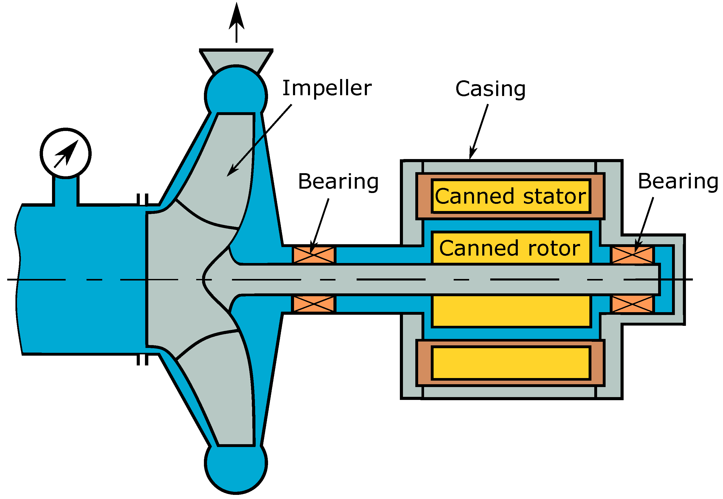
There are other applications where torque losses in the bearings have a significant impact on machine efficiency e.g., pumps for a special purpose. They are mainly used for pumping hazardous liquids Figure 1. Their design takes into account both flooded bearings as well as motor. The pumps are generally designed without seals because they can be exposed to disproportionate conditions like high temperature, or there is a risk of a chemical reaction between the seals and liquid [6,7,8].
Therefore, this article aims to investigate torque losses in ball bearings operating in water and oil, primarily fully flooded. The goal is to modify the drag coefficient, respectively the friction loss coefficient in SKF’s and Palgrem’s empirical model. The torque loss characteristics will be determined for specific ball bearings too. Three bearing types were selected for the purpose: the ball bearing 61820, 6015, and 6210. The bearings were selected because pump prototypes are available with this type of bearing.
2. The Methodology of Torque Loss Determination
The torque loss was determined by combination of two methods, specifically experimental research and numerical simulations (CFD).
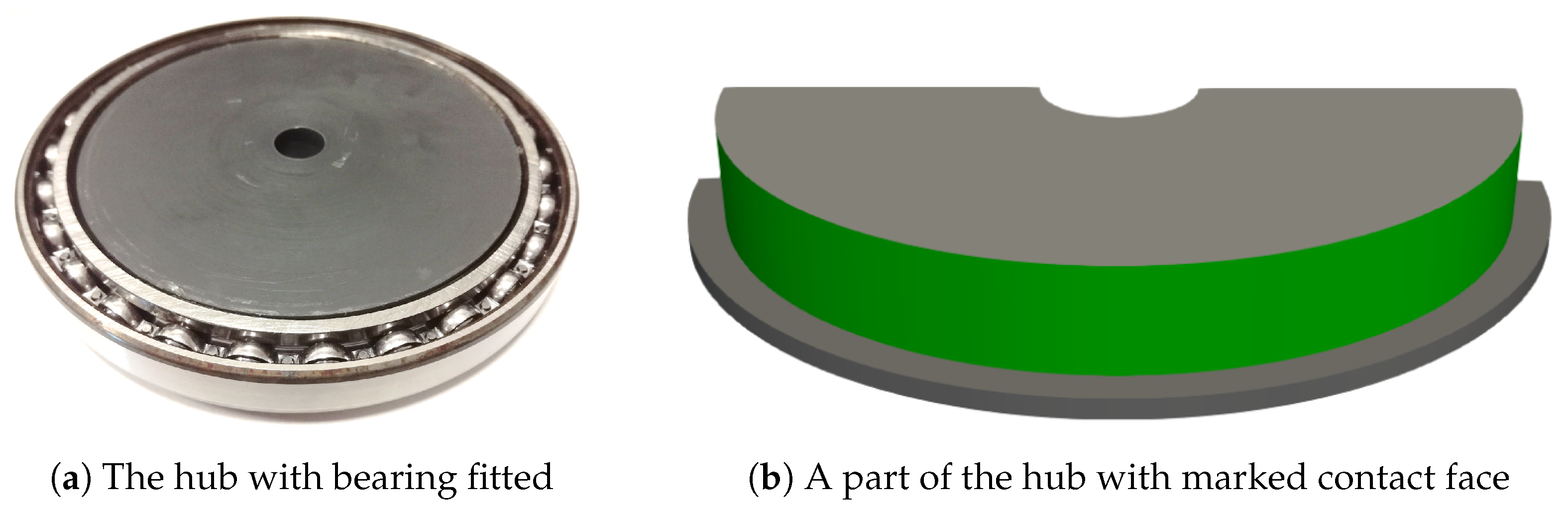
The experimental part of the work had two subtasks. Firstly, torque loss on hubs had to be determined. After that, bearings were fitted to hubs and the measurement was repeated. The final torque loss in bearing was defined as:
where is the measured value of hub with bearing fitted Figure 2a, is the measured value of the hub only and is the torque loss correction on the face (green marked in Figure 2b) used for fitting the bearing. This correction is based on CFD results.
3. Experimental Measurement
The testing campaign was done with bearings which were listed in Table 1.
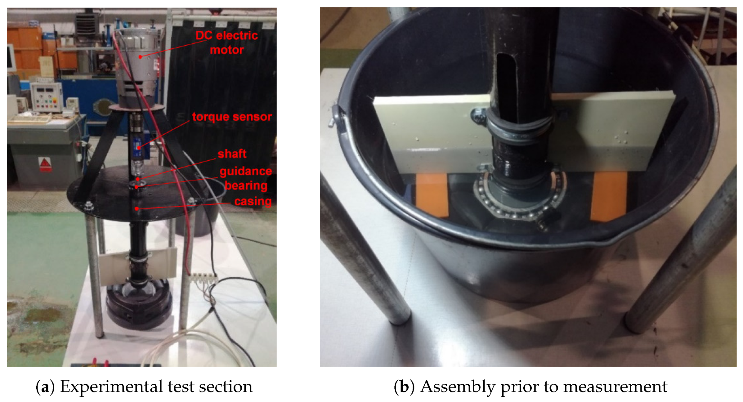
The experimental test section, which consisted of a DC electric motor, DC power supply, PC card for laboratory measurement, casing, shaft and guidance bearings, is shown in Figure 3a. The motor was connected by the shaft to the torque sensor that measured the torque and the rotor speed. One guidance bearing (radial type) was placed on top of the shaft under the torque sensor. The second guidance bearing (sliding type) was placed at the bottom of the case above the hub. The shaft was terminated with the thread. It enabled connection with the hub where the measured bearing was fitted. Motor revolutions were regulated by voltage settings on the DC power supply. In Figure 3b, the measurement assembly was prepared. Additionally, there was a ring that secured the outer ring of the ball bearing against turning. The ring was assembled from the case, and an inner tube was placed inside the case. Due to air pressure regulation in inner tube, the outer ring of the ball bearing could be fixed. The case with the inner tube was pressed into the bucket (Figure 3b); also there were two stationary blades that prevented water from overflowing outside the bucket.
Measurement was performed in range from 500 rpm to 4500 rpm (Actually, there was a limitation in maximal revolutions, because the maximal current load of the motor was 32 A. Therefore, it was impossible to maintain specified revolutions range especially during measurements of bearings 61820 and 6015 in oil.). The step on the revolutions was 500 rpm. An additional point at 100 rpm was included. Bearings were tested in water first. After that, they were dried, and measurement was repeated using oil (ISO VG 46) instead. During measurement, water temperature corresponded to room temperature, thus 20 °C. In contrast, temperature of oil raised to 28 °C and sustained. Therefore viscosity and density of oil were determined for 28 °C.
Data were measured until revolutions torque and temperature of liquids were stabilized. The sampling frequency was 2 kHz and the time interval for data collection was 5 s. So, values of revolutions are average values per s period. LabView software was used for data recording.
The torque sensor with a range of 1 Nm was used during measurement in water. The absolute uncertainty of the device was 0.005 Nm. However, when bearings were measured in oil, it was necessary to use the torque sensor with a higher range, specifically with a range of 20 Nm and the absolute uncertainty of 0.04 Nm. Originally, measurement in oil was divided into two intervals. In each interval, the corresponding torque sensor was used, so that uncertainty of the measurement was reasonable to an absolute value of the measured torque. However, there was a problem to cover uniform conditions during measurement. The changes in oil properties were observed after air was mixed in. Additionally, it was not possible to ensure the same mechanical conditions (tolerances, etc.), when the torque sensor was exchanged. Because of that, measurement in oil was finally done with torque sensor to 20 Nm in order to run measurement fast and to limit these negative phenomena.
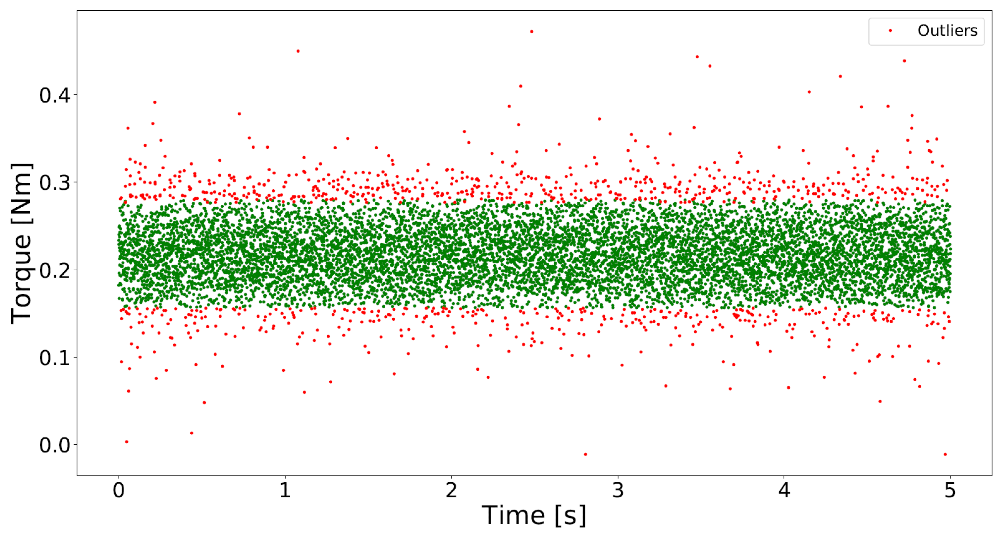
After preliminary result files were checked, some outliers were found. These had to be ruled out. The normal distribution test (Shapiro–Wilk) was done, but hypotheses were rejected. So outliers could not be ruled out, assuming the normal distribution. Therefore i-forest (i-forest—isolation forest algorithm is an unsupervised learning algorithm for anomaly detection.) [9] algorithm was applied (Figure 4). When outliers were ruled out, then average values for appropriate revolutions were determined. The resulting average values were approximated by the least square method. Equations, which were obtained in previous step, were used to recalculate the torque loss to the nominal value of revolutions e.g., 500 rpm.
4. Determination of Torque Losses Correction on the Hub by CFD
As mentioned in the previous section, CFD analysis was made because it was necessary to determine torque loss on the face corresponding to the contact face between the hub and the ball bearing. This way, it was possible to determine the final torque loss in ball bearing as the difference between torque measurement in ball bearing including the hub and torque measurement in hub.
CFD analysis was carried out in OpenFoam 6 [10]. Dimensions of hubs and their geometry are presented in Figure 5a and Table 2. In Figure 5b, there is the scheme of the domain that was used in the CFD simulation.
All meshes were made in the BlockMesh utility and they were consisted only of hexahedral. Due to the symmetry of geometry, it was possible to employ only one half of the domain. The simpleFoam and pimpleFoam solvers were used for steady-state and transient cases, respectively. In all simulations, the k- SST turbulence model was used. Mechanical properties of a liquid that were applied in simulations are listed in Table 3.
The steady-state cases were solved first. Compared to the experiment, only half of the domain was used and cyclic boundary conditions were applied. Rotating wall velocity was prescribed on rotating faces to match the nominal value of revolutions in the experiment. The effect of the liquid-free surface was neglected compared to the experiment as it was replaced by the slip wall boundary condition. Due to the poor convergence behaviour, the schemes were set as follows: Gauss upwind as divergence scheme for momentum and turbulence terms, with Gauss linear scheme for gradient terms. The condition of maximal y+ = 1 for the k- SST model has been met on rotational faces in the domain.
As the steady-state cases did not give satisfactory results, after comparison with measurement the transient analyses were computed in selected cases. The time step was set form to s according to revolutions. Cases were initialized from steady-state results. After several iterations, divergence schemes were changed to the second-order (Gauss linear).
Results from CFD analysis were processed as follows. On the face of interest, percentage torque loss was determined, where a sum of the torque loss over the whole rotor is 100%. Thanks to this percentual torque loss (PTL) that was determined for each value of revolutions, it was possible to set on corrected torque loss in hub. Corrected torque loss in hub was determined after averaging the PTL over revolution for specific hub’s geometry. From the CFD results (Table 4 and Table 5), it was possible to confirm the assumption that PTL is not a function of revolution.
5. Results
The dependence of the torque loss in ball bearings on revolutions is presented in Figure 6, Figure 7 and Figure 8. Every figure contains results for oil and water for the specified ball bearings. The order of polynomials that were selected for the interpolation of measurement points is quadratic. It was chosen according to the dynamic similarity of hydraulic machines where the quadratic dependence of the torque on revolutions is assumed.
PTL that were determined in CFD on the face of interest (see Section 2.) are listed in Table 4 for water and Table 5 for oil. Torque losses in “hub”, presented in Figure 6, Figure 7 and Figure 8, already include the torque loss correction. The absolute uncertainty for oil measurement is 0.04 Nm and for water measurement 0.005 Nm.
In cases where oil was used as a fluid, it was difficult to determine the character of flow, respectively to determine the Reynolds number. There is no strictly prescribed formula for Reynolds number, especially if the distance between surface of the hub and surface of the bucket is considerable. Thus, the test was made on geometry of the hub, where laminar flow was assumed. However, results did not differ significantly (Table 5 and Table 6).
The resulting dependence of the friction coefficient from Palmgren’s model on revolutions is in Figure 9. A similar dependence is shown in Figure 10 for the drag loss factor from the SKF model.
Figure 9 and Figure 10 show, that coefficient respectively coefficient are a function of the revolutions. This conclusion is in contradiction to the literature [2,3,4], which assumes that these coefficients are independent of revolutions, respectively they are constant on the range of the revolutions. Note that the same results were obtained for other types of tested bearings and fluids.
6. Discussion
The torque loss characteristics in selected types of ball bearings were determined. As it was mentioned, it was impossible to reach higher revolutions in ball bearings 61820 and 6015 during measurement in oil due to the current limitation in the motor.
Time-dependent results () were tested to the normal distribution, and hypotheses were rejected. It was probably caused by averaging data over the measurement period respectively by the selected sampling frequency.
Measurement of bearings and hubs in the oil had several issues. Firstly, oil viscosity is highly dependent on the temperature. The oil temperature was checked on the free surface, but there are doubts about equal distribution of the temperature in the whole volume, mainly between inner and outer rings of bearings. After the measurement campaign, the oil was foamed and saturated by air. The air bubbles mixed in oil could have certainly affected the torque estimation. Therefore, measurement with oil was done using one torque sensor in order to run measurement quickly and to limit these negative phenomena. Thus, bigger absolute uncertainty (0.04 Nm) was noticed during measurement in oil, compared to measurement in water, where it could be possible to use torque sensors with a range to 1 Nm with an absolute uncertainty of 0.005 Nm.
For CFD simulations, it was assumed that hubs surfaces were ideally smooth without any roughness. Neglecting the surface roughness in simulation could have influenced the results even though the surface on the physical model was relatively smooth. The influence of turbulent models is discussed in the article [11], where a similar type of geometry was solved. After consideration, some aspects as computational time, mesh quality requirement, and fact that CFD simulation was only used to relative torque loss estimation, k- SST turbulence model was chosen.
As it was mentioned in the results section, a test where laminar flow in oil was assumed during CFD simulation was performed. However, the results almost did not differ from cases where the turbulence model was used (Table 5 and Table 6).
In the end, there was an effort to determine coefficient in Palmgren’s model (Figure 9) and drag loss factor in SKF model (Figure 10). The dependence of the coefficients on revolutions is obvious from mentioned figures, which is in contradiction to the literature [2,3,4], where they are assumed as constant on the range of the revolutions. However, the literature references do not assume fully flooded bearing. As a result of the above, it is impossible to determine the general drag coefficient for a specific bearing type.
There is a new gap for research that can aim to determine new an empirical model for torque loss in flooded bearing which is beyond the scope of this article. There is also a gap to improve the methodology of the friction torque loss estimation and to generalize torque loss results. For example, turbulence models -SST [12] or kv2- [13] can be used, because they are suitable for transition boundary layer modeling. Additionally, the influence of the radial force acting on bearings could be examined.
Author Contributions
Methodology, M.D. and J.Z.; writing—original draft preparation, M.D.; writing—review and editing, V.H. and J.T. All authors have read and agreed to the published version of the manuscript.
Funding
This research was funded by project “Computer Simulations for Effective Low-Emission Energy Engineering” funded as project No. CZ.02.1.01/0.0/0.0/16_026/0008392 by Operational Programme Research, Development and Education, Priority axis 1: Strengthening capacity for high-quality research and by specific research project of FSI VUT No. FSI-S-20-6235.
Institutional Review Board Statement
No human subjects, human material, human tissues or human data were involved in the presented research.
Informed Consent Statement
Not applicable.
Data Availability Statement
The data that support the findings of the study are available from the corresponding author upon reasonable request.
Acknowledgments
Project “Computer Simulations for Effective Low-Emission Energy Engineering” funded as project No. CZ.02.1.01/0.0/0.0/16_026/0008392 by Operational Programme Research, Development and Education, Priority axis 1: Strengthening capacity for high-quality research and specific research project of FSI VUT No. FSI-S-20-6235.
Conflicts of Interest
The authors declare no conflict of interest.
References
- Gülich, J.F. Centrifugal Pumps, 2nd ed.; Springer: Berlin/Heidelberg, Germany, 2010. [Google Scholar] [CrossRef]
- Wiemer, M. Theoretische und Experimentelle Untersuchungen zum Betriebsverhalten voll Rolliger Zylinderrollenlager. Ph.D. Dissertation, Univ., Fak. f. Maschinenwesen, Hannover, Germany, 1990. [Google Scholar]
- Harris, T.A. Rolling Bearing Analysis, 4th ed.; John Wiley: Hoboken, NJ, USA, 2001; ISBN 0-471-35457-0. [Google Scholar]
- The SKF Model for Calculating the Frictional Moment. Available online: https://www.skf.com/binaries/pub12/Images/0901d1968065e9e7-The-SKF-model-for-calculating-the-frictional-movement_tcm_12-299767.pdf (accessed on 29 March 2021).
- Abdan, S.; Stosic, N.; Kovacevic, A.; Smith, I.; Asati, N. Analysis of rolling bearing power loss models for twin screw oil injected compressor. IOP Conf. Ser. Mater. Sci. Eng. 2019. [Google Scholar] [CrossRef] [Green Version]
- Optimex. Available online: https://www.optimex-pumps.com/sealless-canned-motor-pump-technology/canned-motor-principle/ (accessed on 4 May 2021).
- KSB. Available online: https://www.ksb.com/centrifugal-pump-lexicon/canned-motor/192464/ (accessed on 4 May 2021).
- SPA. Available online: https://www.starpumpalliance.com/canned-motor-pumps (accessed on 4 May 2021).
- Liu, F.T.; Ting, K.M.; Zhou, Z.H. Isolation Forest. In Proceedings of the 2008 Eighth IEEE International Conference on Data Mining, Pisa, Italy, 15–19 December 2008. [Google Scholar] [CrossRef]
- OpenFOAM. Available online: https://openfoam.org/version/6/ (accessed on 13 April 2021).
- Zemanová, L.; Rudolf, P. Turbulence Models for Simulation of the Flow in a Rotor-Stator Cavity. In EPJ Web of Conferences; EDP Sciences: Les Ulis, France, 2018. [Google Scholar] [CrossRef]
- Menter, F.R.; Smirnov, P.E.; Liu, T.; Avancha, R. A One-Equation Local Correlation-Based Transition Model. Flow Turbul. Combust. 2015. [Google Scholar] [CrossRef]
- Lopez, M.; Walters, D.K. Prediction of transitional and fully turbulent flow using an alternative to the laminar kinetic energy approach. J. Turbul. 2015. [Google Scholar] [CrossRef]
Figure 1.
Canned motor pump.

Figure 2.
The assembly of the hub and the bearing.

Figure 3.
Experimental measurement.

Figure 4.
Ball bearing 61820 measured data for water at 2000 rpm after the outliers elimination.

Figure 5.
Geometry of the hub and computational domain.

Figure 6.
Bearing 61820—Torque losses in water and oil.

Figure 7.
Bearing 6015—Torque losses in water and oil.

Figure 8.
Bearing 6210—Torque losses in water and oil.

Figure 9.
Bearing 61820 water— coefficient—Palmgren’s model.

Figure 10.
Bearing 61820 water— drag loss factor—SKF model.


Table 1.
List of ball bearings with outer () and inner () diameters.
| Type of Bearings | (mm) | (mm) |
|---|---|---|
| 61820 | 125 | 100 |
| 6015 | 115 | 75 |
| 6210 | 90 | 50 |
Table 2.
Hub dimensions.
| 61820 | 6015 | 6210 | |
|---|---|---|---|
| A (mm) | 100 | 75 | 50 |
| B (mm) | 15 | 24 | 23.8 |
| C (mm) | 2.3 | 4.8 | 4.5 |
| D (mm) | 109 | 90 | 71 |
Table 3.
Liquid mechanical properties.
| Density (kg/m3) | Kinematic Viscosity (m2/s) | |
|---|---|---|
| Water | 998.2 | |
| ISO VG 46 | 857.8 |
Table 4.
Results of transient CFD simulations for hubs in water.
| 500 rpm | 2500 rpm | 4500 rpm | ||||
|---|---|---|---|---|---|---|
| Type of Bearings | Total Torque CFD (Nm) | PTL (%) | Total Torque CFD (Nm) | PTL (%) | Total Torque CFD (Nm) | PTL (%) |
| 61820 | 0.011556 | 20.02 | 0.206424 | 20.68 | 0.607270 | 20.72 |
| 6015 | 0.005519 | 22.23 | 0.095071 | 23.55 | 0.285224 | 24.06 |
| 6210 | 0.001941 | 17.09 | 0.031173 | 17.39 | 0.089743 | 16.94 |
Table 5.
Results of transient CFD simulations for hubs in oil.
| 500 rpm | 2500 rpm | 4500 rpm | ||||
|---|---|---|---|---|---|---|
| Type of Bearings | Total Torque CFD (Nm) | PTL (%) | Total Torque CFD (Nm) | PTL (%) | Total Torque CFD (Nm) | PTL (%) |
| 61820 | 0.067487 | 15.30 | 0.774147 | 13.90 | 1.887112 | 13.84 |
| 6015 | 0.033710 | 19.78 | 0.397034 | 17.30 | 0.975630 | 18.94 |
| 6210 | 0.013495 | 15.65 | 0.0.150078 | 13.06 | 0.370136 | 15.72 |
Table 6.
Results of the transient CFD simulations for the hub 61820 in oil if laminar flow is assumed.
Table 6.
Results of the transient CFD simulations for the hub 61820 in oil if laminar flow is assumed.
| Revolution (rpm) | Total Torque CFD (Nm) | PTL(%) |
|---|---|---|
| 500 | 0.065853 | 16.19 |
| 2500 | 0.766787 | 13.46 |
| 4500 | 1.865688 | 13.42 |
Publisher’s Note: MDPI stays neutral with regard to jurisdictional claims in published maps and institutional affiliations. |
© 2021 by the authors. Licensee MDPI, Basel, Switzerland. This article is an open access article distributed under the terms and conditions of the Creative Commons Attribution (CC BY) license (https://creativecommons.org/licenses/by/4.0/).
Share and Cite
MDPI and ACS Style
Dobrovolný, M.; Habán, V.; Tancjurová, J.; Zbavitel, J. An Investigation of Viscous Torque Loss in Ball Bearing Operating in Various Liquids. Water 2021, 13, 1414. https://doi.org/10.3390/w13101414
AMA Style
Dobrovolný M, Habán V, Tancjurová J, Zbavitel J. An Investigation of Viscous Torque Loss in Ball Bearing Operating in Various Liquids. Water. 2021; 13(10):1414. https://doi.org/10.3390/w13101414
Chicago/Turabian StyleDobrovolný, Martin, Vladimír Habán, Jana Tancjurová, and Jan Zbavitel. 2021. "An Investigation of Viscous Torque Loss in Ball Bearing Operating in Various Liquids" Water 13, no. 10: 1414. https://doi.org/10.3390/w13101414
Note that from the first issue of 2016, this journal uses article numbers instead of page numbers. See further details here.