Moment Analysis for Modeling Soil Water Distribution in Furrow Irrigation: Variable vs. Constant Ponding Depths

Abstract

Despite increasing use of pressurized irrigation methods, most irrigation projects worldwide still involve surface systems. Accurate estimation of the amount of infiltrating water and its spatial distribution in the soil is of great importance in the design and management of furrow irrigation systems. Moment analysis has previously been applied to describe the subsurface water distribution using input data from numerical simulations rather than field measured data, and assuming a constant ponding depth in the furrow. A field experiment was conducted in a blocked-end level furrow at Maricopa Agricultural Center, Arizona, USA, to study the effect of time-variable ponding depths on soil water distribution and the resulting wetting bulb under real conditions in the field using moment analysis. The simulated volumetric soil water contents run with variable and constant (average) ponding depths using HYDRUS 2D/3D were almost identical, and both compared favorably with the field data. Hence, only the simulated soil water contents with variable ponding depths were used to calculate the moments. It was concluded that the fluctuating flow depth had no significant influence on the resulting time-evolving ellipses. This was related to the negligible 10-cm variation in ponding depths compared to the high negative matric potential of the unsaturated soil.

1. Introduction

Gravity-flow (or surface) irrigation has been referred to as “wasteful”, “primitive”, or “inefficient”, and many farms have switched to pressurized systems [1]. Despite increasing use of pressurized irrigation methods, most irrigation projects worldwide still involve surface systems. Walker and Skogerboe [2] noted that surface irrigation methods were favored over sprinkler, trickle, and subirrigation methods due to lower capital and operating costs, the simplicity of maintenance, and the utility of unskilled labor. Strelkoff et al. [3] stated that for low-value crops, and where pressurized irrigation was not easy to adopt, surface irrigation was likely to be practiced on a significant portion of irrigated lands for the foreseeable future. Sanchez et al. [4] mentioned high installation costs of pressurized systems, salinity build up with subsurface drip irrigation, complicated crop rotations, and the differing needs with regard to cultural practices as limitations to the general adoption of drip irrigation. They stated that for the foreseeable future, furrow irrigation would remain the principal method of irrigation for vegetable crops in the Lower Colorado River region (LCRR). About two-thirds of Arizona farms rely on gravity irrigation on about 88% of irrigated acres. In Arizona, most farms rely on border/basin control, but most of the acres are irrigated by furrows [1].

An accurate estimation of the amount of water that enters the soil and its spatial distribution has proved to be important in the design and management of furrow irrigation systems. The subsurface water distribution depends on soil hydraulic properties, initial soil water content, flow depth, furrow geometry, and crop and climatic factors. Lazarovitch et al. [5] proposed moment analysis to describe the evolving wetting patterns from drip emitters at a constant flow rate. The required data were obtained from infiltration simulations run in a two-dimensional domain with surface line or buried cylindrical cavity sources, and a three-dimensional axially symmetric domain in HYDRUS-2D. They stated that this approach could accurately describe the water content distribution with just three indices: the vertical center of gravity, and the standard deviation in the horizontal and vertical directions. Lazarovitch et al. [6] implemented moment analysis to describe the spatial and temporal subsurface water distribution during infiltration and redistribution from a furrow. As with Lazarovitch et al. [5], this was done by only calculating the location of the center of the plume and the lateral and vertical spreading of water about its mean position. Numerical simulations were conducted with HYDRUS-2D in three contrasting soils to generate the required data to compute the moments. They concluded that moment analysis could accurately approximate the general shape of the wetted volume. Lazarovitch et al. [7] modeled soil water distribution from trickle emitters using artificial neural networks (ANNs). The database developed with HYDRUS-2D was used to examine the usefulness of three different schemes: water contents at specified coordinates, spatial moments, and coordinates of water content contours. Results suggested that moment analysis was probably the most successful method to describe soil water distribution. Following Lazarovitch et al. [7], Hinnell et al. [8] designed an Excel-based ANN called Neuro-Drip to describe the spatio-temporal distribution of the infiltrated water from a surface drip emitter. It could also estimate the time when the center of mass equals a given value and the corresponding wetted soil pattern using inverse analysis. Spatial and temporal moments were calculated using the results from many different infiltration simulations run with HYDRUS. The ANN was tested by estimating the depth to the center of mass and the vertical and radial spreading of water based on soil hydraulic properties and the discharge rate as the input. This approach was found to be very flexible, providing fast and easy predictions under the studied conditions. Sperling and Lazarovitch [9] used moment analysis to evaluate the two-dimensional wetting patterns from a dripper source during and after infiltration in a laboratory experiment conducted in two contrasting soils. Continuous images of the soil were taken by a color scanner and then transformed into soil water content values. The calculated moments could simply and efficiently describe the soil water distribution.

To describe the subsurface water distribution from furrows, Lazarovitch et al. [6] merely derived the moments with input data from numerical simulations rather than field measured data, and assuming a constant ponding depth in the furrow. However, flow depths are variable in the field. To extend the previously published study by Lazarovitch et al. [6], the authors of the present study were interested in taking into account the effect of variations in ponding depth at the infiltrating surface on soil water distribution and how that would influence the development of the resulting wetting bulb under real conditions in the field. To this end, a field experiment was conducted at Maricopa Agricultural Center (MAC) to collect the data that would be used to compute the moments with variable ponding depths.

2. Materials and Methods

2.1. Field Experiment

The Maricopa Agricultural Center (MAC) is a University of Arizona research and demonstration farm. The farm is 770 hectares in size with an elevation of 358 m from standard sea level. This study was conducted on a Trix soil reclaimed and classified as a fine-loamy, mixed (calcareous), hyperthermic Typic Torrifluvents. Typically, this soil has a clay loam or sandy clay loam surface horizon that is 0–30 cm deep. The upper subsurface horizon ranges from 30 to 100 cm deep, and it has similar characteristics as the surface horizon.

Table 1. Selected characterization data for the study farm.

Field	Soil Mapping Unit Symbol	Textural Class	Depth (cm)	Sand (%)	Clay (%)	BD (g·cm−3)
18	TR	Clay loam	0–70	25–45	27–40	1.4–1.55

summarizes the selected characterization data for the farm. Since the ranges are given, an average of the two values was used for sand (%) = 35, clay (%) = 33.5, silt (%) = 31.5, and BD (g·cm⁻³) = 1.5.

In order to produce spatial and temporal flow depth variations, a blocked-end level furrow with two buffer furrows on each side were prepared. Every other furrow receives wheel traffic when being listed and shaped. The test was conducted on a non-wheel furrow with a symmetric trapezoidal cross-section on a total length of 100 m and a row spacing of 1.02 m. The furrow geometry including top and bottom width and maximum depth was measured at five locations along the furrow and averaged (

Table 2. Furrow geometry.

Parameter	Unit	Value
Furrow length (L)	m	100
Furrow spacing (FS)	cm	102
Bottom width (BW)	cm	7
Top width (TW)	cm	52
Maximum depth (hmax)	cm	12
Side slope (SS)	cm·cm−1	1.88
Average bed slope (S0)	m·m−1	−0.00013

).

Prior to irrigation, initial soil water content samples were taken along the experimental furrows and averaged. Water was delivered to the test furrows using a gated pipe at an inflow rate of 1.89 L·s⁻¹ (30 gpm) per furrow. The experimental and buffer furrows were equipped with a flume to record accurate measurements of the inflow. It took about 10 min for the inflow to reach a constant rate. The inflow reached the downstream end at t_L = 36.58 min and it was cut-off at t_co = 77 min. We used large heads to achieve quick completion of advance in zero slope furrows. The quick advance allows for better application and distribution efficiency. We would have topped the furrow if we did not cut-off when we did [4]. The experiment continued until almost the whole water content had receded (infiltrated) (t_r = 124 min) and was well into the redistribution (t = 100 h).

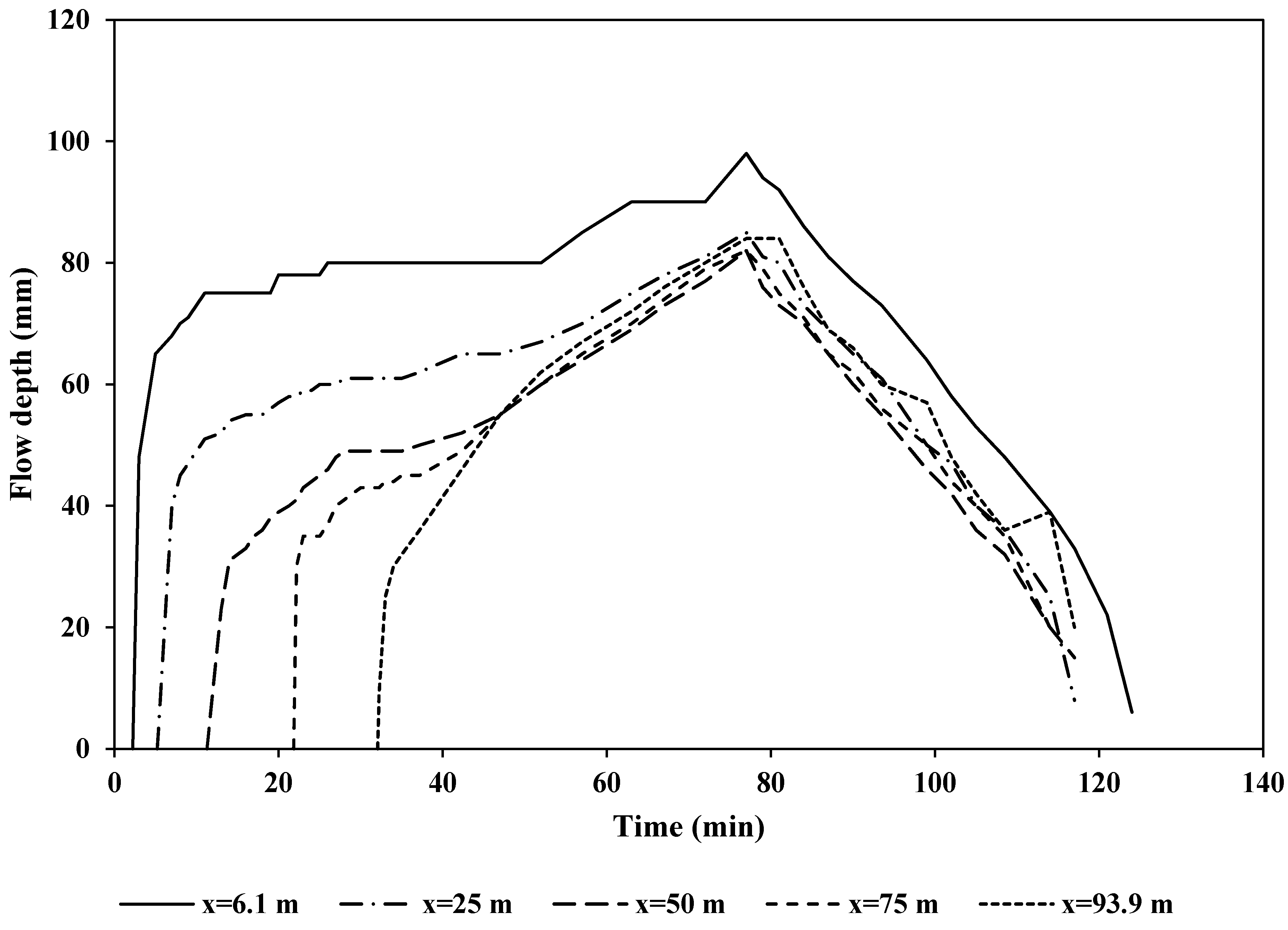
During the irrigation event, data were collected on the inflow rate, and the advance and recession times for the five stations along the furrow. Surface flow depth readings were taken at regular spatial (25 m apart) and temporal intervals until near recession using staff gauges instrumented at each station. Figure 1 depicts the resulting water depth hydrographs at five stations downstream from the furrow inlet (at 6.1, 25, 50, 75, and 93.9 m). The moisture profile was measured only once in the redistribution phase. Soil moisture samples were collected from the soil surface through a depth of 105 cm (in 15-cm increments) below the center of the furrow bed and ridge after 99, 99.5, and 100 h after the onset of irrigation at stations 1, 3, and 5, respectively. The corresponding surface flow depth information for the three stations is summarized in

Table 3. Corresponding data for the depth hydrographs at three stations along the test furrow.

Station	Position (m)	Arrival Time (min)	Peak Depth (mm)	Average Depth (mm)
1	6.1	2.23	96	72
3	50	11.27	82	53
5	93.9	32.07	84	59

. As can be seen from the hydrographs in Figure 1, initially there is a rise in depth as the surface water reaches a station until a peak depth (near normal depth) is attained before stabilization. Then, because of the backwater effect, the water level starts to rise above the normal depth until it declines following the inflow cutoff. The rising phase is very slow in comparison with the decline phase. Whereby, the average depth was nearly 75%, 65%, and 70% of the peak depth for stations 1, 3, and 5, respectively.

2.2. Numerical Computations

The subsurface flow of water in this study was simulated using HYDRUS 2D/3D, previously shown to successfully simulate the two-dimensional subsurface water flow from irrigation furrows (e.g., Ebrahimian et al. [10], Deb et al. [11], Šimůnek et al. [12], Liu et al. [13], and Bristow et al. [14]).

The HYDRUS software (version 1.xx)package numerically solves the Richards’ equation for saturated-unsaturated water flow and convection-dispersion-type equations for heat and solute transport. Subsurface water flow from a furrow irrigation experiment is a two-dimensional process. The “$h$-based” form of the Cartesian Richards’ equation for two dimensions is:

$$C_w\left(h\right)\frac{\partial h}{\partial t}=\frac{\partial }{\partial x}\left(K\left(h\right)\frac{\partial h}{\partial x}\right)+\frac{\partial }{\partial z}\left(K\left(h\right)\frac{\partial h}{\partial z}\right)-\frac{\partial K\left(h\right)}{\partial z}$$

(1)

where $C_w\left(h\right)$ is the soil water (or hydraulic) capacity function $\left[{\mathrm{L}}^{-1}\right]$; $h$ is the soil matric head $\left[\mathrm{L}\right]$; $K\left(h\right)$ is the hydraulic conductivity $\left[{\mathrm{LT}}^{-1}\right]$; $t$ is time $\left[\mathrm{T}\right]$; $x$ is the horizontal coordinate $\left[\mathrm{L}\right]$; and $z$ is the vertical coordinate, positive downwards $\left[\mathrm{L}\right]$. The van Genuchten–Mualem model (Mualem [15], van Genuchten [16]) was used to describe the soil hydraulic properties in the Richards’ equation:

$$\theta \left(h\right)=\{\begin{array}{cc}{\theta }_r+\frac{{\theta }_s-{\theta }_r}{{\left[1+{\left|\alpha h\right|}^n\right]}^m},& h<0\\ {\theta }_s,& h\ge 0\end{array}$$

(2)

$$K\left(h\right) = K_s{S}_e^l{\left[1-{(1-S_e^{1/m})}^m\right]}^2$$

(3)

with

$$\begin{array}{ccc}m = \frac{1}{n},& n>1,& S_e = \frac{\theta -{\theta }_r}{{\theta }_s-{\theta }_r}\end{array}$$

(4)

where $\theta$ is the volumetric water content [L³L⁻³]; ${\theta }_r$ is the residual volumetric water content $\left[{\mathrm{L}}^3{\mathrm{L}}^{-3}\right]$; ${\theta }_s$ is the saturated volumetric water content $\left[{\mathrm{L}}^3{\mathrm{L}}^{-3}\right]$; $K_s$ is the saturated hydraulic conductivity [LT⁻¹]; $S_e$ is the relative water content or effective saturation $[-]$; $\alpha$ is the inverse of the air-entry value (or bubbling pressure) $\left[{\mathrm{L}}^{-1}\right]$; $n$ is a pore size distribution index $[-]$; and $m$ is a pore connectivity parameter [–], for which a value of 0.5 is used as an average for many soils. The hydraulic properties of the soil were predicted using Rosetta (Schaap et al. [17]) and are summarized in

Table 4. The van Genuchten–Mualem hydraulic properties for the test soil.

Parameter	θr	θs	α	n	l
Unit	cm3·cm−3	cm3·cm−3	cm−1	-	-
Value	0.0788	0.4142	0.0136	1.3817	0.5

.

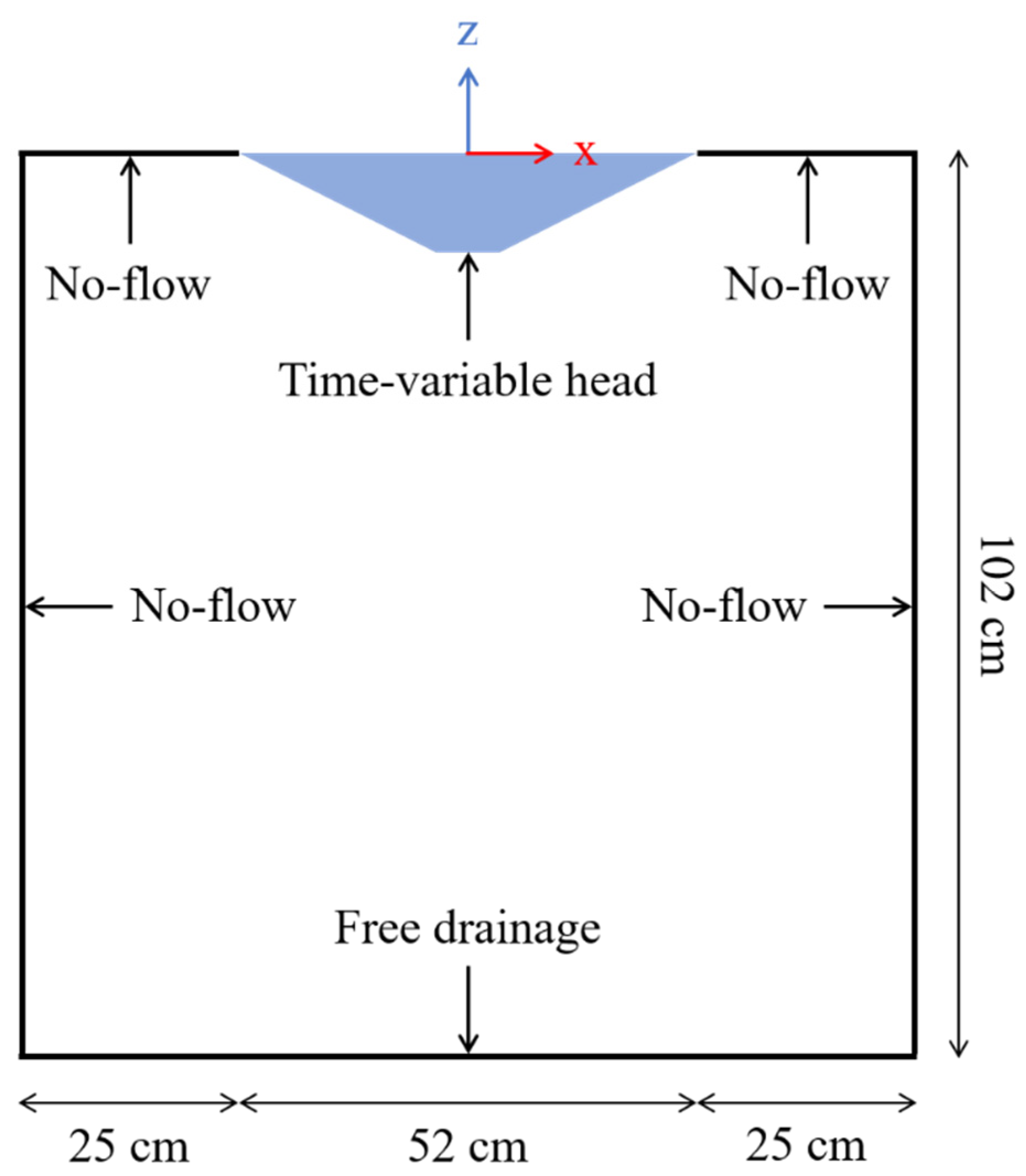
The computational flow domain depicted in Figure 2 is 102 × 102 cm and is discretized into 1897 nodes with smaller finite elements around the furrow. An average initial volumetric soil water content of 0.13 is specified on the entire domain. Irrigation is initiated by ponding the furrow. The upper time-variable pressure head boundary condition is assigned to represent the fluctuating water level in the furrow. It remains variable/constant during irrigation and changes to atmospheric boundary condition during redistribution. The lower boundary is set to free drainage.

2.3. Moment Analysis

The two-dimensional spatial moments for moisture plume [18] are defined as

$$M_{ik}={\int }_{-\infty }^{+\infty }{\int }_{-\infty }^{+\infty }{\theta }_{\mathrm{diff}}\left(x,z,t\right)x^i{z}^{k}dxdz$$

(5)

where ${\theta }_{\mathrm{diff}}\left(x,z,t\right)=\theta \left(x,z,t\right)-{\theta }_{\mathrm{i}}\left(x,z,t\right)$ is the water content at a given time; $t$ at a location $x,z$; ${\theta }_{\mathrm{i}}\left(x,z,t\right)$ is the background water content; $x$ and $z$ are the levers from the z- and x-axes, respectively; and $i, k$ are indices of 0, 1, or 2. The zeroth moment, $M_{00}$ is equal to the volume of water applied to the domain. The first moments, $M_{10}$ and $M_{01}$, are used to calculate the location of the center of the plume.

$$x_C=\frac{M_{10}}{M_{00}}$$

(6)

$$z_C=\frac{M_{01}}{M_{00}}$$

(7)

The second moments, $M_{20}$ and $M_{02}$, relate to the amount of spreading about its mean position in the x and z directions (${\sigma }_x^2\left[{\mathrm{L}}^2\right]$ and ${\sigma }_z^2\left[{\mathrm{L}}^2\right]$) [19].

$${\sigma }_x^2=\frac{M_{20}}{M_{00}}-x_C^2$$

(8)

$${\sigma }_z^2=\frac{M_{02}}{M_{00}}-z_C^2$$

(9)

2.4. Data Processing

HYDRUS simulations were run for the three stations along the test furrow with constant and variable ponding depths. The measured water depth hydrographs at the three stations down the furrow inlet (at 6.1, 50, and 93.9 m) were used as the upper time variable boundary condition in HYDRUS for the variable ponding depth scenarios. For the constant ponding depth scenarios, these values were averaged in time at each station and the resulting constant value was used as the upper boundary condition. The obtained soil water contents from simulations were then used to calculate $M_{ik}$, $z_C$, ${\sigma }_x$, and ${\sigma }_z$ for a given time using Equations (5)–(9). The $x_C$ was assumed to be zero due to symmetry. An equally spaced grid was defined to compute the moments. A square area was assigned to each observation point, inside which the water content was assumed to be constant and equal to the water content of the closest finite element node to that observation point. Once the moments were computed, time-evolving ellipses around the center of mass (0,$z_C$) were defined using $s{\sigma }_x$ and $s{\sigma }_z$, where $s$ is the number of standard deviations.

$$\frac{x^2}{s^2{\sigma }_x^2}+\frac{z^2}{s^2{\sigma }_z^2}=1$$

(10)

The fraction of applied water contained within an ellipse was calculated as a ratio of the mass of applied water retained in an ellipse to $M_{00}$. By repeating the calculations for increasing values of $s$, larger ellipses containing percentages of the applied water can be calculated. The corresponding cumulative probability function increases from zero to one as $s$ becomes large enough that the corresponding ellipse contains nearly the total applied water [5,6].

3. Results and Discussion

3.1. Numerical Computations

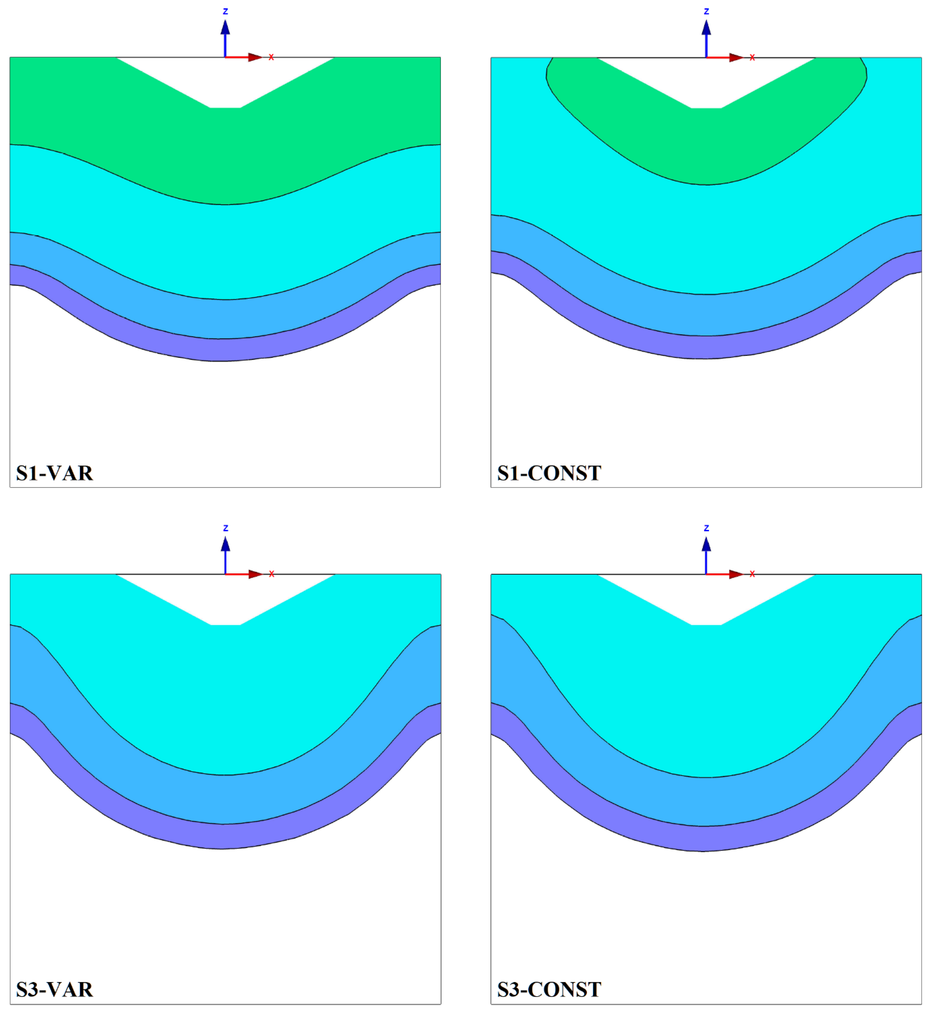
Simulated volumetric soil water contents for the variable head as well as the constant (average) head at a station were compared to each other and to the field-measured data collected at various measurement points within a furrow. The resulting wetting patterns are presented in Figure 3 and the corresponding volumetric soil water contents as well as the field-measured soil moisture data are given in

Table 5. Observed (OBS) and simulated volumetric soil water content with variable (VAR) and constant (CONST) ponding depth at a station.

Depth (cm)	Bed						Station	Ridge
	12–27	27–42	42–57	57–72	72–87	87–102		0–15	15–30	30–45	45–60	60–75	75–90	90–102
							S1
OBS	0.18	0.18	0.26	0.19	0.16	0.15		0.16	0.18	0.18	0.15	0.14	0.14	0.17
VAR	0.24	0.23	0.22	0.18	0.14	0.13		0.24	0.23	0.21	0.16	0.13	0.13	0.13
CONST	0.24	0.23	0.22	0.18	0.13	0.13		0.23	0.22	0.20	0.15	0.13	0.13	0.13
							S3
OBS	0.17	0.19	0.18	0.17	0.14	0.12		0.15	0.17	0.18	0.13	0.12	0.11	0.13
VAR	0.23	0.22	0.20	0.16	0.13	0.13		0.21	0.20	0.16	0.13	0.13	0.13	0.13
CONST	0.23	0.22	0.20	0.16	0.13	0.13		0.21	0.19	0.16	0.13	0.13	0.13	0.13
							S5
OBS	0.15	0.19	0.17	0.13	0.19	0.15		0.13	0.15	0.16	0.13	0.11	0.12	0.11
VAR	0.22	0.22	0.20	0.15	0.13	0.13		0.20	0.19	0.15	0.13	0.13	0.13	0.13
CONST	0.22	0.22	0.20	0.15	0.13	0.13		0.19	0.17	0.14	0.13	0.13	0.13	0.13

. Interestingly, there was a perfect fit between the simulations run with variable and constant ponding depths with an RMSE value of 0.01 and a correlation coefficient of 0.99 for the entire furrow. Additionally, both simulations compared favorably with the field experiment. Very close average RMSE values of 0.04 and 0.03 were obtained for the entire furrow comparing observations to the simulations run with the variable and constant ponding depths, respectively.

3.2. Moment Analysis

Since the simulated volumetric soil water contents and the resulting wetting bulbs were almost identical using the variable or constant ponding depths, the moments were only calculated using variable ponding depths at $t$ = 1, 1.5, 6, and 60 for all three stations and at a total time of 99, 99.5, or 100 h for stations 1, 3, and 5, respectively.

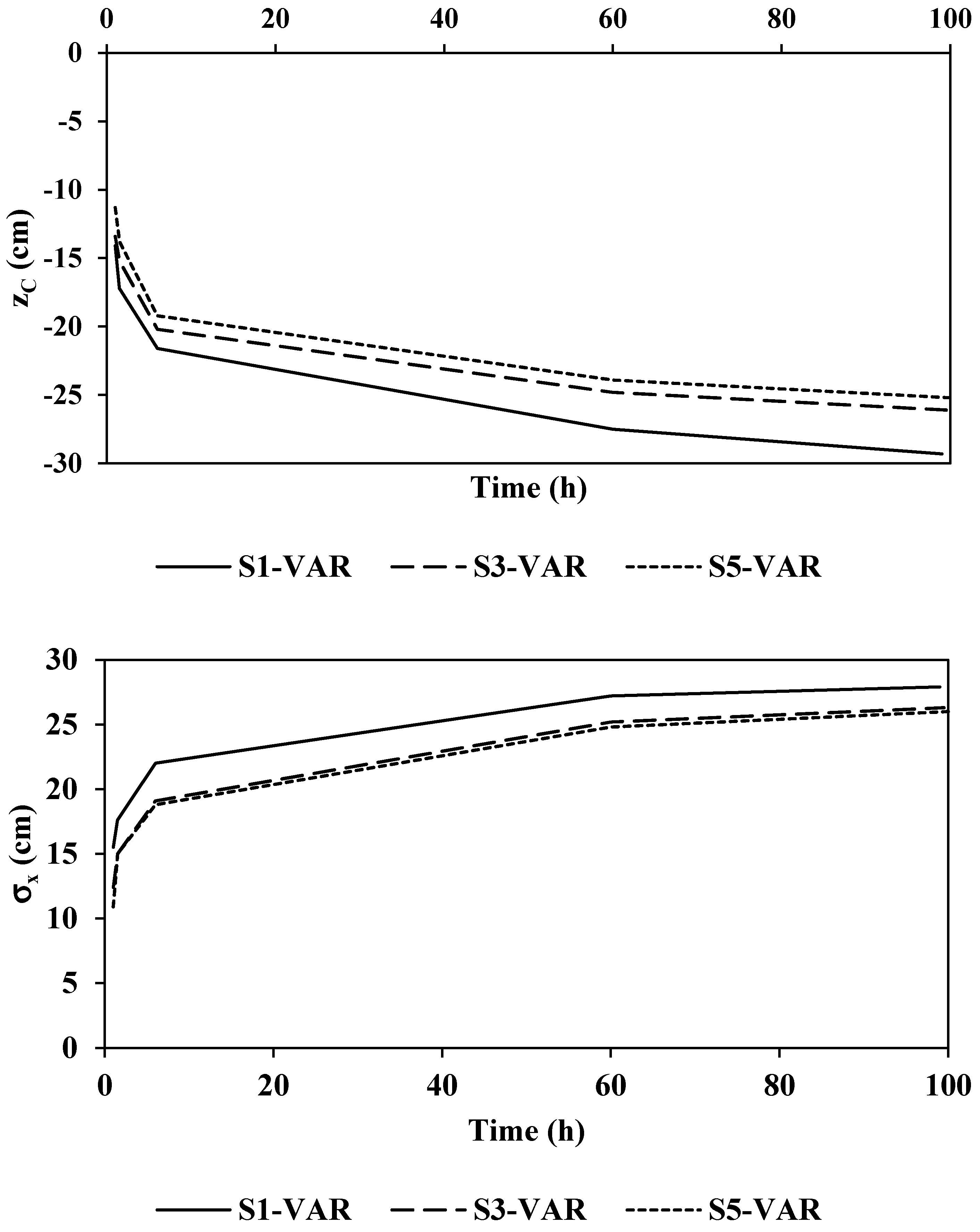
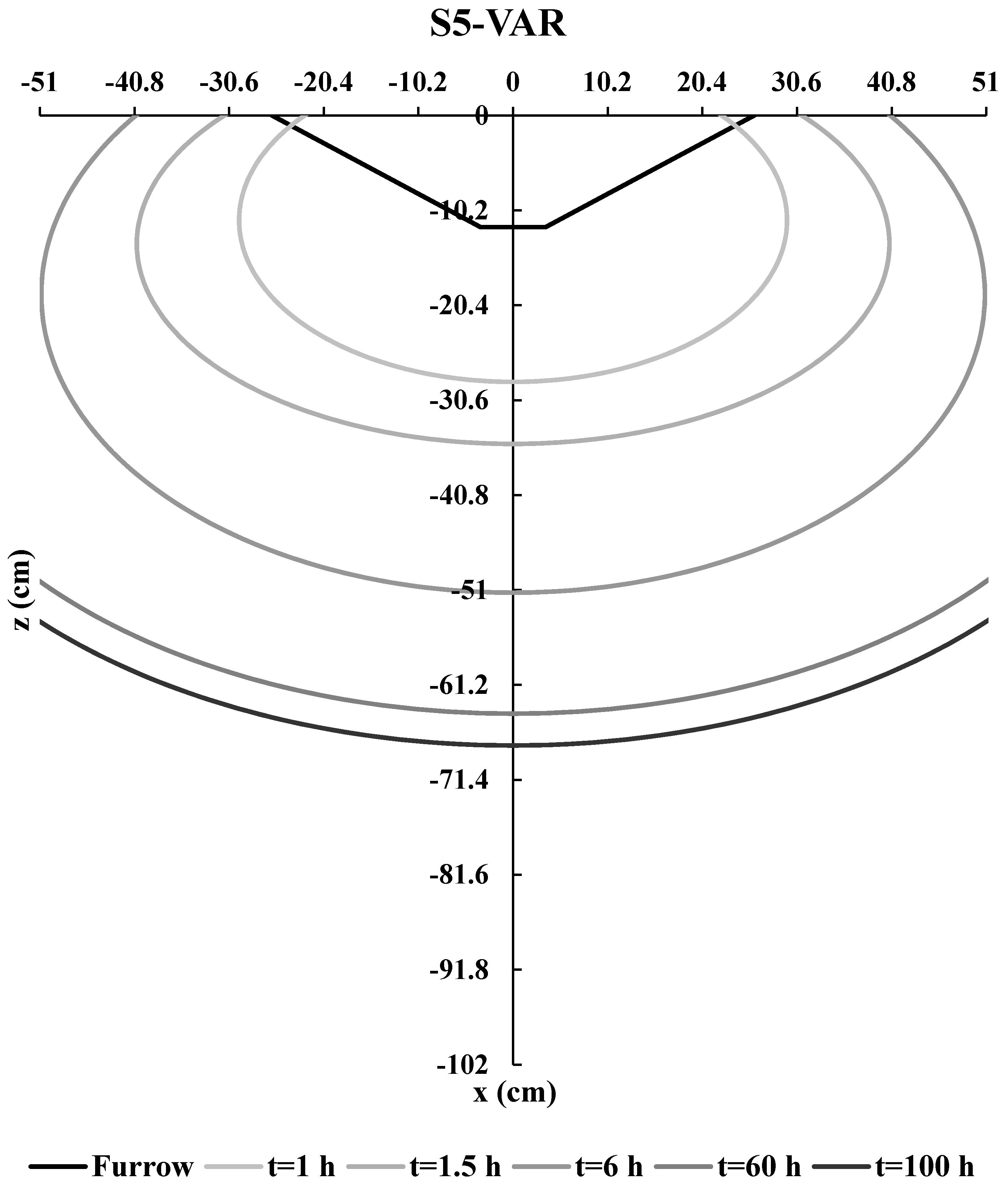
As explained earlier, increasing the size of the ellipses defined by moment analysis is attained by using a larger $s$ value. Using $s$ = 2.7 for stations 1 and 5, and $s$ = 2.6 for station 3, nearly all the applied water resided within all the time-evolving ellipses. The resulting location of the center of mass, $z_C$, and the semi-axes of the ellipses, ${\sigma }_x$ and ${\sigma }_z$ for the variable head calculations are depicted in Figure 4. It can be seen from Figure 4 that the downward movement of the center of mass was fast during infiltration, gradually slowed as water advanced deeper into the soil profile, and remained almost constant during redistribution. The $z_C$ was the deepest for station 1 because water ponded there for a longer time. Similar to $z_C$, ${\sigma }_x$ and ${\sigma }_z$ changed very quickly initially, and were slower after several hours. The corresponding values for $z_C$, ${\sigma }_x$, and ${\sigma }_z$ are given in

Table 6. The location of the center of mass, $z_C$, and the semi axes of the ellipses, ${\sigma }_x$ and ${\sigma }_z$, with variable (VAR) ponding depth at stations 1 (S1), 3 (S3), and 5 (S5).

Time (h)	S1-VAR					S3-VAR					S5-VAR
	1	1.5	6	60	99	1	1.5	6	60	99.5	1	1.5	6	60	100
$z_C$ (cm)	−14.1	−17.2	−21.6	−27.5	−29.3	−13.4	−15.2	−20.2	−24.8	−26.1	−11.3	−13.8	−19.2	−23.9	−25.2
${\sigma }_x$ (cm)	15.5	17.6	22.0	27.2	27.9	12.4	15.0	19.1	25.2	26.3	10.9	15.0	18.8	24.8	26.0
${\sigma }_z$ (cm)	8.2	10.5	13.2	17.1	18.1	7.8	9.2	12.4	15.4	16.4	6.4	8.0	11.9	14.9	15.7

. Moreover, the resulting plots of the ellipses are presented in Figure 5 for the variable head calculations at a station. The ellipses were elongated in the horizontal direction which is consistent with the expected wetting patterns in a clay loam soil.

Gravity and matric potential dominate the energy of water under unsaturated conditions. In dry soils, the matric potential head is so negative that it often dominates the effect of gravity [19]. The recorded peak ponding depth in the test furrow herein was 9.6 cm at station 1. Most of the hydraulic gradient driving the water into the soil stems from the high negative pore pressures in the unsaturated soil ahead of the wetting front. Hence, the effect of variations in the ponding depth in the range of 0 to 10 cm on infiltration rates, and therefore on the resulting wetting patterns (the computed ellipses), is negligible. This is in accord with early empirical studies of the water depth effect, evaluating field techniques of measuring infiltration rates or studying infiltration during irrigation, which are most concerned with shallow water depths in the range from 0 to 20 cm, and suggest that the depth effect is small [20]. It is expected that if there was any difference, it would be more pronounced with lighter soils where water tends to percolate more rapidly. Hence, it is highly recommended to extend the current study to various soil textures with contrasting hydraulic properties.

Moreover, as with Hinnell et al. [8] for drip irrigation, a machine learning framework such as artificial neural networks can be used as future work to package a large volume of irrigation water distribution data using the results of moment analysis directly estimated from the soil and geometric properties, without the need to conduct simulations with HYDRUS 2D/3D.

4. Conclusions

A field experiment was conducted in a blocked-end level furrow at Maricopa Agricultural Center (MAC) to take into account the effect of time-variable ponding depths at the infiltrating surface. The moments were calculated using the simulated soil water contents with HYDRUS 2D/3D using variable ponding depths in three stations along the test furrow. It was concluded that the fluctuating flow depth had no significant influence on the resulting time-evolving ellipses. This was related to the negligible 10-cm variation in ponding depths compared to the high negative matric potential of the unsaturated soil. We expect that there would be pronounced differences in more coarse-textured soils than that used in this evaluation, and additional studies over a range of soil textures are warranted. Furthermore, the results of moment analysis can be used as future work to package a large database that could be used to estimate irrigation water distribution using a machine learning framework, such as artificial neural networks, without the need to conduct simulations with HYDRUS 2D/3D.

References

- Frisvold, G.; Sanchez, C.A.; Gollehon, N.; Megdal, S.B.; Brown, P. Evaluating Gravity-Flow Irrigation with Lessons from Yuma, Arizona, USA. Sustainability 2018, 10, 1548. [Google Scholar] [CrossRef] [Green Version]
- Walker, W.R.; Skogerboe, M. Surface Irrigation: Theory and Practice; Prentice-Hall: Englewood Cliffs, NJ, USA, 1987; p. 386. [Google Scholar]
- Strelkoff, T.S.; Clemmens, A.J.; El-Ansary, M.; Awad, M. Surface-irrigation evaluation models: Application to level basins in egypt. Trans. ASAE 1999, 42, 1027–1036. [Google Scholar] [CrossRef]
- Sanchez, C.A.; Zerihun, D.; Farrell-Poe, K.L. Management guidelines for efficient irrigation of vegetables using closed-end level fur-rows. Agric. Water Manag. 2009, 9, 43–52. [Google Scholar] [CrossRef]
- Lazarovitch, N.; Warrick, A.W.; Furman, A.; Šimunek, J. Subsurface Water Distribution from Drip Irrigation Described by Moment Analyses. Vadose Zone J. 2007, 6, 116–123. [Google Scholar] [CrossRef] [Green Version]
- Lazarovitch, N.; Warrick, A.W.; Furman, A.; Zerihun, D. Subsurface Water Distribution from Furrows Described by Moment Analyses. J. Irrig. Drain. Eng. 2009, 135, 7–12. [Google Scholar] [CrossRef]
- Lazarovitch, N.; Poulton, M.; Furman, A.; Warrick, A.W. Water distribution under trickle irrigation predicted using artificial neural networks. J. Eng. Math. 2009, 64, 207–218. [Google Scholar] [CrossRef]
- Hinnell, A.C.; Lazarovitch, N.; Furman, A.; Poulton, M.; Warrick, A.W. Neuro-Drip: Estimation of subsurface wetting patterns for drip irrigation using neural networks. Irrig. Sci. 2010, 28, 535–544. [Google Scholar] [CrossRef]
- Sperling, O.; Lazarovitch, N. Characterization of Water Infiltration and Redistribution for Two-Dimensional Soil Profiles by Moment Analyses. Vadose Zone J. 2010, 9, 438–444. [Google Scholar] [CrossRef]
- Ebrahimian, H.; Liaghat, A.; Pasinejad, M.; Abbasi, F.; Navabian, M. Comparison of one- and two-dimensional models to simulate al-ternate and conventional furrow fertigation. J. Irrig. Drain. Eng. 2012, 138, 929–938. [Google Scholar] [CrossRef]
- Deb, S.K.; Sharma, P.; Shukla, M.K.; Ashigh, J.; Šimůnek, J. Numerical Evaluation of Nitrate Distributions in the Onion Root Zone under Conventional Furrow Fertigation. J. Hydrol. Eng. 2016, 21, 05015026. [Google Scholar] [CrossRef] [Green Version]
- Šimůnek, J.; Bristow, K.L.; Helalia, S.A.; Siyal, A.A. The effect of different fertigation strategies and furrow surface treatments on plant water and nitrogen use. Irrig. Sci. 2016, 34, 53–69. [Google Scholar] [CrossRef] [Green Version]
- Liu, K.; Huang, G.; Xu, X.; Xiong, Y.; Huang, Q.; Šimůnek, J. A coupled model for simulating water flow and solute transport in furrow irrigation. Agric. Water Manag. 2019, 213, 792–802. [Google Scholar] [CrossRef] [Green Version]
- Bristow, K.L.; Šimůnek, J.; Helalia, S.A.; Siyal, A.A. Numerical simulations of the effects furrow surface conditions and fertilizer loca-tions have on plant nitrogen and water use in furrow irrigated systems. Agric. Water Manag. 2020, 232, 1–11. [Google Scholar] [CrossRef]
- Mualem, Y. A new model for predicting the hydraulic conductivity of unsaturated porous media. Water Resour. Res. 1976, 12, 513–522. [Google Scholar] [CrossRef] [Green Version]
- Van Genuchten, M.T. A Closed-form Equation for Predicting the Hydraulic Conductivity of Unsaturated Soils. Soil Sci. Soc. Am. J. 1980, 44, 892–898. [Google Scholar] [CrossRef] [Green Version]
- Schaap, M.G.; Leij, F.J.; van Genuchten, M.T. Rosetta: A computer program for estimating soil hydraulic parameters with hierarchical pedotransfer functions. J. Hydrol. 2001, 251, 163–176. [Google Scholar] [CrossRef]
- Yeh, T.-C.J.; Ye, M.; Khaleel, R. Estimation of effective unsaturated hydraulic conductivity tensor using spatial moments of observed moisture plume. Water Resour. Res. 2005, 41, W03014. [Google Scholar] [CrossRef]
- Radcliffe, D.; Šimůnek, J. Soil Physics with HYDRUS: Modeling and Applications; CRC Press, Taylor & Francis Group: Boca Raton, FL, USA, 2010; p. 388. [Google Scholar]
- Lewis, M.R.; Powers, W.L. A Study of Factors Affecting Infiltration. Soil Sci. Soc. Am. J. 1939, 3, 334–339. [Google Scholar] [CrossRef]
Figure 1.
Measured flow depth hydrographs at five stations along the test furrow. “x” is the distance from the furrow inlet.
Figure 2.
Flow domain and the assigned boundary conditions.
Figure 3.
Simulated soil wetting patterns with variable (VAR) and constant (CONST) ponding depth at stations 1 (S1), 3 (S3), and 5 (S5). Volumetric soil water contents (cm3·cm−3) are denoted by th [-].
Figure 4.
The location of the center of mass, , and the semi axes of the ellipses, and , with variable (VAR) ponding depth at stations 1 (S1), 3 (S3), and 5 (S5).
Figure 5.
The time-evolving ellipses with variable (VAR) head calculations at stations 1 (S1), 3 (S3), and 5 (S5).