
Automatic Calibration Module for an Urban Drainage System Model


Department of Civil Engineering and Architecture, Tallinn University of Technology, Ehitajate tee 5, 19086 Tallinn, Estonia
*
Author to whom correspondence should be addressed.
Water 2021, 13(10), 1419; https://doi.org/10.3390/w13101419
Submission received: 13 April 2021
/
Revised: 13 May 2021
/
Accepted: 17 May 2021
/
Published: 19 May 2021
(This article belongs to the Special Issue Urban Drainage Systems in Smart Cities)
Abstract
:The purpose of the study was to present an automated module for the calibration of urban drainage system models. A prepared tool based on the Open Water Analytics toolkit included 12 additional calibration parameters as compared to the existing similar solutions. The module included a gradient optimization method that allowed adjustment of up to five parameters simultaneously, and a trial-and-error method that provided the possibility of testing one or two parameters. The user interface was built in MS Excel to simplify use of the developed tool. The user can select preferable parameters for calibration, choose the optimization method, and determine the limits for the calculated values. The performance and functionality of the automatic calibration module was tested in two scenarios using the drainage model of a 10 ha heavily developed area in Tallinn, Estonia. The calibration results revealed that the maximum deviation between the modelled and measured flow rates was less than 5% for both cases. This is a reasonably good fit for drainage models, which typically encounter numerous uncertainties. Therefore, it was concluded that the module can be successfully used for calibrating hydraulic models created in SWMM5.
1. Introduction
Climate change is having a considerable impact on urban areas [1], bringing more extreme rainfall events [2,3]. The intensities of the extreme rainfalls have increased more than 30%, as measured by rain gauges in Tallinn during the last five years, and are exceeding design thresholds of design standards. This means that existing urban drainage systems (UDS) might be incapable of handling the increasing volumes, resulting in surcharge and consecutive pluvial floods. According to [4,5], rapid urban development will accelerate the risk of floods even more, as densification typically increases the ratio of impermeable surfaces and disrupts the natural water cycle. Therefore, a substantial shift in the paradigm of urban drainage design, planning and operation is needed. “Smart” drainage systems, i.e., real time controlled (RTC) facilities that emerged with the development of information and communication technology (ICT), and integration of low impact development (LID) solutions, have the potential to make the needed changes [6]. Modelling helps to understand and minimize various sources of uncertainties (e.g., flow rate, rainfall data, runoff) and gain information on how the catchment responds to different rainfall events [7]. Further, numerical modelling is the primary tool for assessing alternative design plans and their effect on urban drainage operation [8]. It is recognized that flood risk mitigation in urban areas relies on the accuracy of supercritical flow representation that can be offered by a numerical model that simulates fluid dynamics [9]. Moreover, RTC of a drainage system depends directly on the existence of calibrated and validated hydraulic models [6].
A typical hydraulic model of the existing UDS contains hundreds or even thousands of pipes and subcatchments, each of these having more than 20 parameters that need to be defined by the users. Site-specific data concerning the structure and geometric properties of a UDS section is often incomplete, thereby hindering the specification of suitable parameters [10]. Most of these cannot be measured directly and providing estimates is a challenge. Therefore, calibration of these parameters becomes crucial in achieving the desired accuracy of the modelling results. At the same time, due to the large number of parameters, calibration poses a major difficulty [11]. A thorough step-by-step overview of the calibration process is presented in [12]. Most of the hydraulic models are calibrated manually [13], which is labour-intensive and presumes in-depth knowledge of the system’s operating conditions. Therefore, automatic calibration (i.e., defining suitable model parameters using optimization algorithms) of a UDS model is suggested to find the values for the key parameters with minimal effort so that the model can accurately predict the response of the physical system, e.g., [13,14,15,16,17,18,19,20]. Jin et al. [14] divided the calibration parameters into two groups: universal parameters that change in a relatively small space, and special parameters that can change in a larger space. The calibration parameters were selected based on the sensitivity study of Barco et al. [16] who showed that the most relevant parameters for model calibration are Manning’s roughness coefficient for conduits, percentage of the impervious surface area, storage depth of the impervious area and width of the subcatchment. Other parameters have smaller effects on the calibration results. Barco et al. [16] used a total of ten storms for calibration and validation, which led to the suggestion that calibration for the average storm is not always appropriate for larger storms. In addition, it has to be considered that a calibration based on a single event can result in significantly different outcomes than for a continuous event. Swathi et al. [15] used eight single rainfall events to calibrate seven individual parameters of the model. Eight calibrated sets were then validated for five continuous rainfalls. Similar to [16], it was concluded that calibration of small magnitude rainfalls was not adequate compared to high magnitude rainfalls [15]. Sensitivity analysis indicated that Manning’s roughness coefficient for catchments and conduits had little impact on the peak flow and runoff volume. The impact of different calibration parameters is clearly case-dependent, as was also shown by Kim et al. [18], who analysed urban flooding in the Seogu portion of Daegu, Korea. Eight candidates were identified for calibration of the hydraulic model of the UDS. Sensitivity studies indicated that only Manning’s roughness coefficient for conduits had a significant effect on the predicted surcharge [18]. The exact parameters and the amount of the parameters to be used in the calibration are dependent on the specific layout of the drainage network and the specification of the catchments.
Automatic calibration of the UDS model is essential when applying hydraulic modelling in the everyday decision-making. Therefore, the calibration procedure has to be simple enough that a specialist in the local municipality or water utility can tweak the model parameters and perform the model calibration without having skills in programming and modelling. Automatic calibration and optimization procedures have been coded in Python [15], Matlab [19], C++ [13], C [21], VBA/Excel [20] etc. Del Giudice and Padulano [20] implemented the GANetXL, an optimization add-in for MS Excel, that was originally developed for water supply networks [22] for the automatic calibration of the hydraulic model. An Excel interface was created for the latter development that allowed set up of computation features and calibration using a Genetic Algorithm (GA) [23]. Unfortunately, the add-in was tested under Microsoft Office 2010 and, according to the developer’s web site, there is no support for the newer versions.
Most of the above-mentioned procedures used some variation of the GA. Vassiljev and Koppel [24] showed that GA is inferior for time-sensitive applications, as the solution process is high in computational cost. Therefore, the first aim of this paper is to demonstrate that the gradient methods like Levenberg-Marquardt algorithm (LMA) [25,26] can be used for the calibration of stormwater models. The LMA is used herein for the calibration of models created in SWMM5 software [27] as this is one of the most widely used models of urban water management in the world [28]. The second aim of the study is to show how to utilize the developed calibration module in MS Excel.
2. Materials and Methods
In the present paper, the term automatic calibration represents an optimization process to find the suitable parameters for the UDS model instead of manually changing the calibration variables and evaluating the results for the optimal solution after each model run. Concurrently, the calibration process still uses measurements and requires selection of suitable calibration parameters.
The automatic calibration tool, hereinafter, called the calibration module, for calibrating stormwater system models presented in this study is based on the SWMM5 and MS Excel software (both 32- and 64-bit versions). MS Excel was selected because it is widely used and does not need specific knowledge of programming compared to other popular software such as Matlab, or programming languages like Python. Both SWMM and MS Excel are widely used by experts in academia, water utilities and local municipalities. Therefore, the implementation and integration of the presented calibration module is possible even for end-users that do not have an expert level knowledge in IT and software development. Nevertheless, successful calibration of hydraulic models requires thorough knowledge and previous experience in the field. Therefore, the implementation of the developed tool assumes competences in hydraulic modelling and prior knowledge on the UDS behavior.
The Open Water Analytics OWA-SWMM Open-Source Library [29] was selected as the basis for the developed calibration module. The OWA Toolkit contains more than 50 additional Dynamic Link Library (DLL) functions compared to the original SWMM5 software [27]. These enable the acquisition of additional information about the system and the ability to change necessary system characteristics during the calculations.
As manual calibration is time-consuming work, it is reasonable to automatize the calibration process using additional DLL and other functions. In order to do that, two main problems must be resolved beforehand; first, what model parameters need to be calibrated, and second, how to calibrate them? The list of the calibration parameters depends first of all on the specific model and sensitivity of the model to changing parameters [16]. For example, when the majority of the watershed surface is pervious, it is necessary to calibrate the characteristics of the soil. In the case of impervious areas, it is necessary to calibrate, for example, the depth of depression storage and Manning’s roughness. A thorough step-by-step description of the calibration process is presented in [12], where a list of parameters recommended to be included in the calibration was compiled (Table 1):
In the case of high groundwater levels and inflows to the system, it is beneficial to include the additional parameters in the calibration listed in Table 2, according to [30].
Only some of the abovementioned parameters are added to the OWA Toolkit. In order to enable automatic calibration of more model parameters, the OWA Toolkit was modified by the authors (Table 3). The dynamic-link library (DLL) of SWMM5 was recompiled to enable changing of the additional parameters during the simulation. The definition file was also changed to have the capability to use DLL in Excel. The parameters listed in Table 1 were added to the DLL. Parameters in Table 2 will be added to the automatic calibration module during the next development phase.
DLL can be used in Excel VBA through declaration commands. The DLL was compiled for both 32- and 64-bit Excel versions. In the case of 64-bit Excel version, the commands were modified by adding “PtrSafe” clause into the declaration and changing the end part of the row. Additional declaration commands can be added to manipulate more parameters during the SWMM simulation.
The SWMM automatic calibration module created by the authors consists of two Excel files. The first one contains the calibration program, and the second one is for measured and modelled data and presenting the results. The calibration procedure is carried out in three steps: (1) setting up the folders, files and data; (2) defining the parameters for calibration and selecting the calibration method; (3) analyzing the results. The step-by-step procedure is presented on the flowchart in Figure 1. The referenced Excel sheets are further described in the next section.
Evaluation of parameters is based on the objective function OF, to be minimized as presented as Equation (1):
where and are the measured and simulated discharge, respectively.
There are a number of optimization algorithms for finding the parameter values for calibration. One of the most popular optimization methods in the last decades has been the GA. In some cases, when optimizing water system models, GA can be very time-consuming [24] and, therefore, alternative methods have been proposed for finding the optimal solution. For example, Koppel and Vassiljev [31] showed that based on the surface of the objective function, gradient methods can also be successfully implemented to find the optimal parameters.
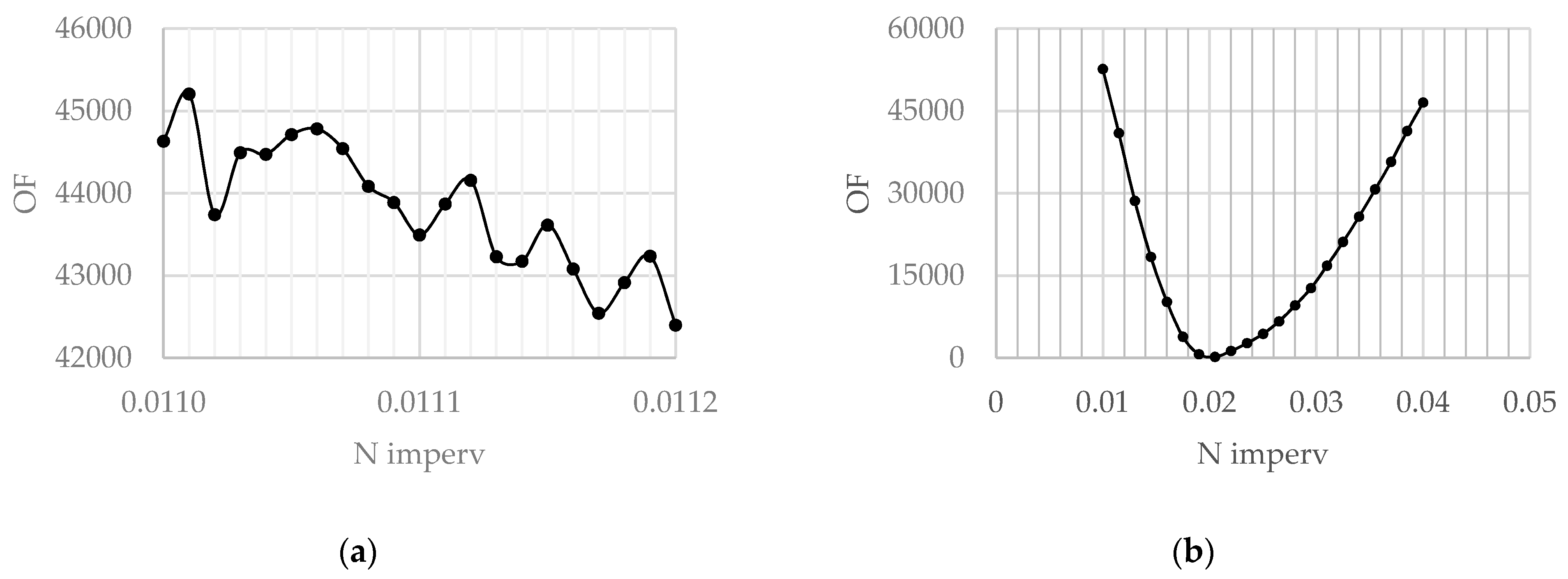
Figure 2a,b present examples of the OF shape when using a different Manning’s roughness coefficient for the overland flow over the impervious areas of an arbitrary drainage system. It is evident from Figure 2a that a very small step in the parameter change leads to a great number of local minimums. This is often a result for hydraulic models with complex layout and a large number of system components. Figure 2b shows that in the case of a larger step, OF changes so that there is only one global minimum when Manning’s roughness coefficient is equal to 0.02. The gradient method finds the nearest minimum; however, in the case of a sufficiently large step, it is also suitable for finding the global minimum. A sensitivity study can be used to find the optimal step for the gradient method. The optimal step is the minimum step along the parameters in case the gradient method can detect the global minimum instead of a local minimum. Dennis, Jr and Schnabel [32] recommended estimation of the size of this step on the basis of the number of reliable digits in the OF values. This can be done by applying Hamming’s method [33], the use of which is described in [34]. The size of the step may also be estimated by trial-and-error, using different step sizes for calculations [31]. A similar approach for analyzing the sensitivity of the parameter step was used in this study.
As was mentioned above, the SWMM5 automatic calibration module consists of two Excel files. The first Excel file of the developed automatic calibration module (i.e., the calibration program) includes the Levenberg-Marquardt algorithm (LMA) for finding the optimal parameter settings in the UDS model calibration for up to five parameters simultaneously. LMA is a gradient method that uses optimization software developed by Argonne National Laboratory (University of Chicago). Minpack package [35], which uses the LMA algorithm, has been rewritten from FORTRAN into Visual Basic and modified slightly to give the user the possibility to change the minimal step along the parameters. In addition to the gradient method (LMA), a trial-and-error method (Surface 21 × 21) was included in the Excel VBA add-on. The latter enables the calculation of the OF for 21 parameter values changing within the user-defined limiting ranges. In this case, up to two parameters can be calibrated simultaneously.
The second Excel file was prepared for data and results and contains the next base sheets:
- Sheet “Surf” where the user-defined parameter ranges used in the calibration need to be inserted. The limits to the parameters can be set according to the user’s preferences, or limit ranges defined in the respective sheet (according to SWMM5 manual). The user can select up to two parameters for the simultaneous calibration using the trial-and-error approach. The results of the OF are presented in a table format on the same sheet.
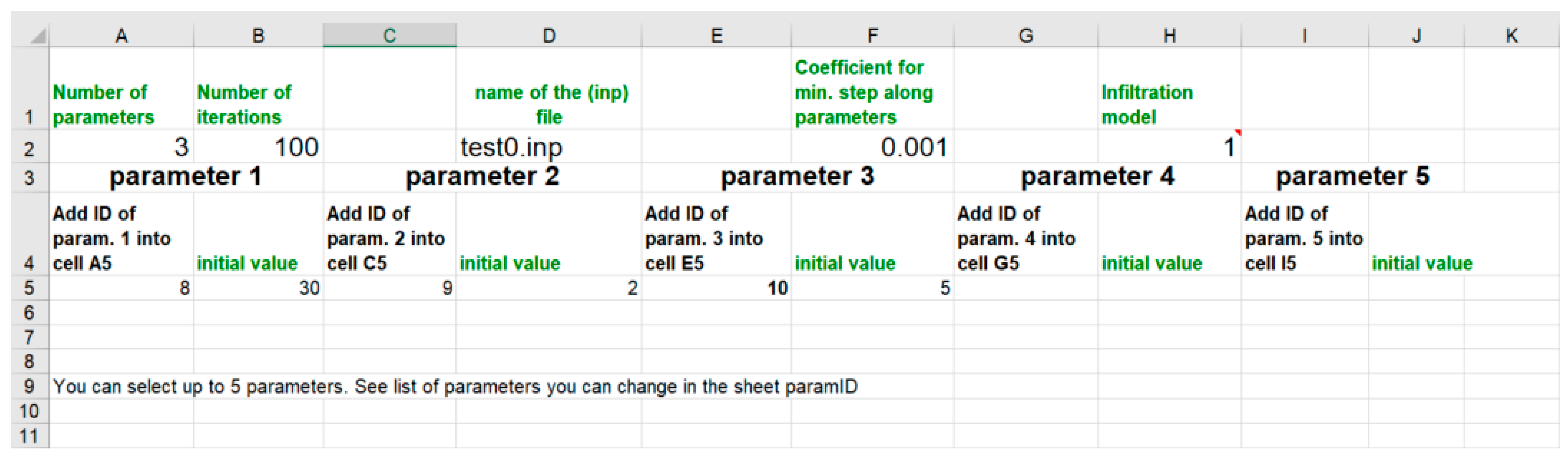
- Sheet “roughLM”, where the user defines the SWMM5 INP file name be used for model calibration, parameter numbers, and initial values of parameters. Up to five different parameters can be defined for simultaneous calibration using LMA. The user interface of the sheet is presented in Figure 3. The parameter ID for parameters 1–5 is defined in a separate sheet paramID.
- Sheet “Measured” contains measurements used in the OF calculations. These can, for example, be measured flow rate at a selected conduit.
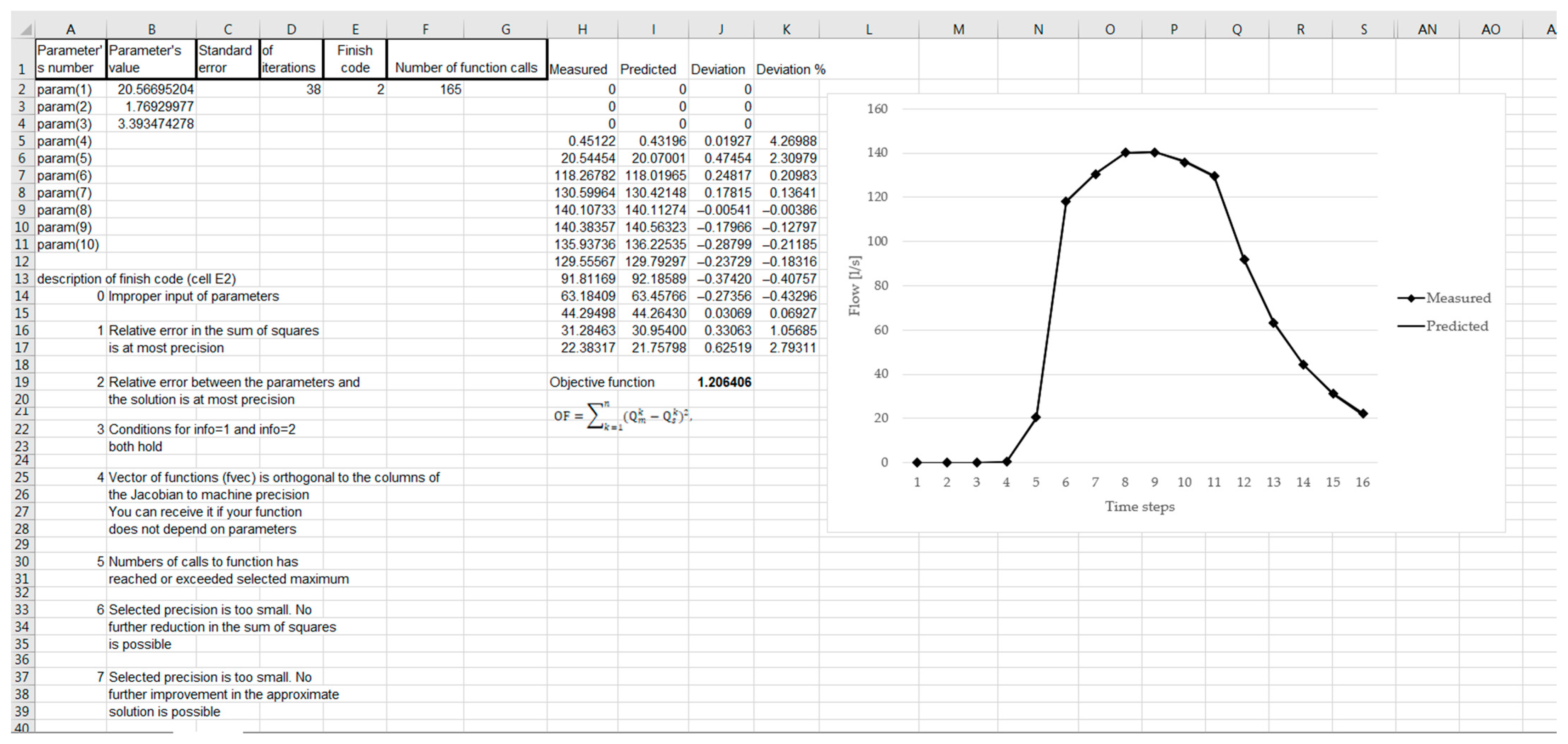
- Sheet “Out_data” presents the calibration results using LMA approach. This includes the final parameter values, deviation of the measured and modelled results, the number of iterations and information about the process defined as finish codes. Seven different finish codes are defined to give the user an instant overview of the calibration procedure. The user’s view of the program is shown in Figure 4.
- Sheet “paramID” contains information about the different parameters that can be included in the automatic model calibration. Each parameter is equipped with an ID, description, and minimal and maximum values. These values can be defined by the user.
Based on the calibration results (Figure 4), the user can decide whether to change the initial values and/or range of the parameters and rerun the calibration or use the proposed values in SWMM for hydraulic simulations.
In addition to the main sheets, the Excel file includes two sheets with parameter limit ranges and error lists, as defined in the SWMM5 manual.
In the Excel workbook, the user cannot change sheet names, or insert rows or columns, because the program reads data from fixed cells. The authors added additional sheets for subcatchments and conduits where the model parameters from the SWMM5 input file are copied. This enables one to update the data after the calibration procedure in the corresponding sheets, and to manually copy the updated parameters to the SWMM5 input file.
3. Results and Discussion
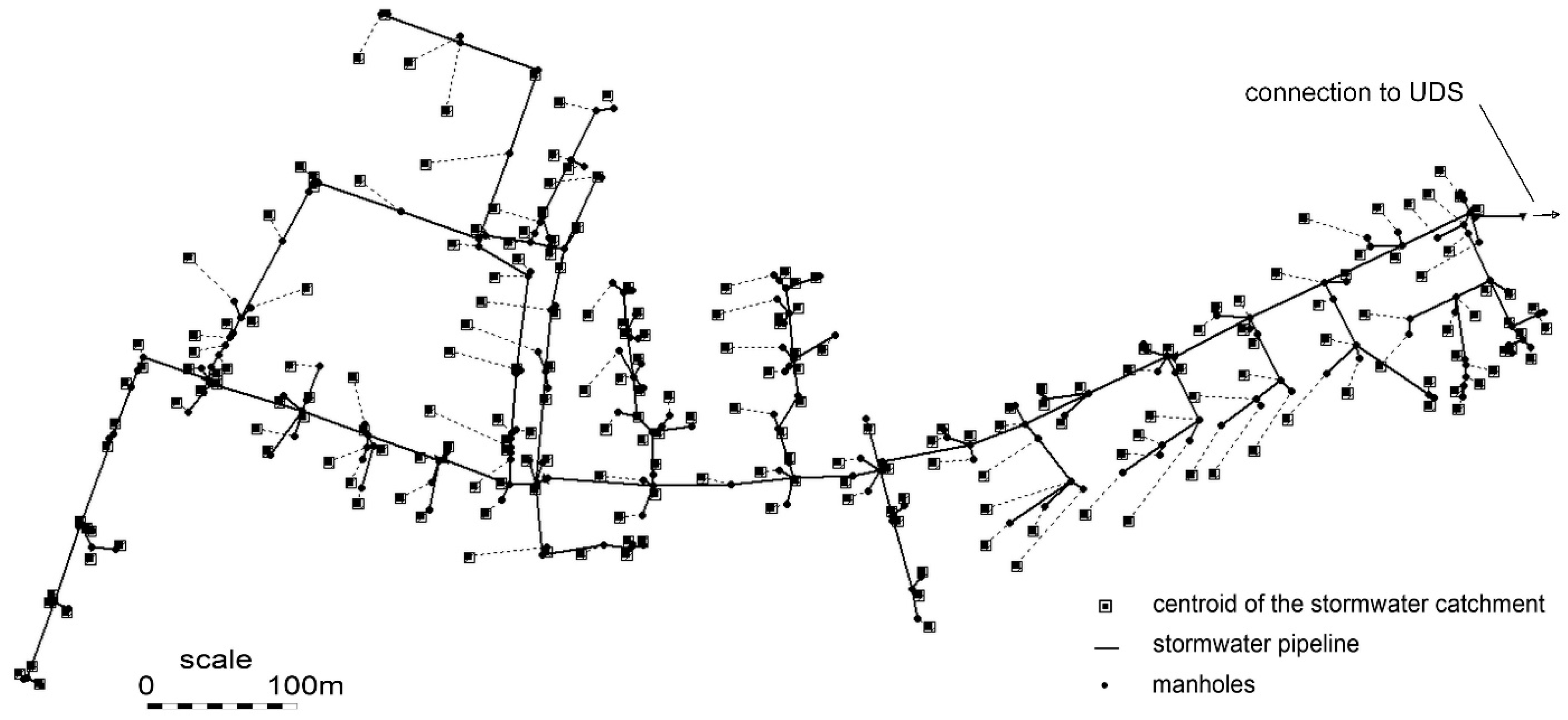
The functionality of the developed Excel-based automatic calibration module was tested on a stormwater model of a large parking area in the city of Tallinn, Estonia. The area, with a ground space of 10.2 ha, is mainly covered with asphalt and cobblestone pavement and is reserved for traffic and parking. The system consists of 222 subcatchments, one for each inlet gully. The total length of the pipeline is 3.5 km, and the diameter of the pipes varies from 0.11 to 0.56 m. The system operates fully on gravity flow and the ground has a moderate 1% slope from east to west. The catchment has one outlet connection to the city’s UDS from where the water is directed to the near-by Baltic Sea (Figure 5).
The properties of the UDS model catchments were artificially changed to mimic systems with different layouts. The OF for different cases under investigation was calculated by comparing the flow rates at the UDS outflow generated by the artificially changed SWMM model (indicated in the text as “Measured”) and the calibrated SWMM model using the developed calibration module (indicated in the text as “Predicted”). This approach allowed checking of the coding in VBA, analysis of the performance of the DLL and testing the functionality of the module.
In this study, two scenarios were analyzed to evaluate the precision of the automatic calibration approach. In the first scenario, the SWMM5 simulation was carried out with catchments defined as 100% impervious. The resulting flow rate at the outlet (indicated as “Measured”) was used in the OF calculations. After that, the imperviousness rate was manually changed in the SWMM5 input file. This file was used for automatic calibration to find the optimal parameters for the Manning’s roughness for the impervious area (N imperv), and the depth of depression storage on the impervious area (Dstore Imperv). In the second scenario, the catchments in the SWMM5 model were defined as 100% pervious. Again, the model was run to find the corresponding flow rates at the outlet. Thereafter, the catchment imperviousness rates were manually changed and the modified input file was used to analyze the reliability and functionality of the developed automatic calibration module. The calibrated parameters in the second scenario were maximum and minimum rate on the Horton infiltration curve (Max. Infil. Rate; Min. Infil. Rate), and the decay constant for the Horton infiltration curve (Decay constant). The objective of the study was to apply the automatic calibration module and to verify the overall functioning of the program. As the rainfall and runoff data for the pilot area were insufficient, the calibration module was tested using the results of the initial model set-up.
Subcatchments for the model were generated automatically using the GisToSWMM5 tool developed in Aalto University [36] The data for the tool was prepared in a Geographic Information System (GIS) based on land use and the digital elevation model (DEM) provided by Corine Land Cover maps and Estonian Land Board data bases. The DEM enables the determination of the slope for each subcatchment automatically. The GisToSWMM5 tool takes the elevation, land-use and flow direction information from the user-prepared input files, creates subcatchment groups for each manhole, and routes the water inside the subcatchments group into the stormwater network through the closest manhole. The precision of the subcatchment generation depends on the resolution of the DEM raster. In this study, a DEM with a grid size of 5 × 5 m was used. The layout with the GisToSWMM5 generated subcatchments for the UDS network used in testing the functioning of the automatic calibration module is presented in Figure 5.
As mentioned above, the user must copy a part of the SWMM input file (containing the parameters to be adjusted during the calibration, such as conduit roughness or subcatchments slope) to the Excel workbook containing the data sheet. The automatic calibration procedure does not change the parameters in the data sheet automatically. Therefore, it is necessary for the user to change the corresponding parameters in the Excel data sheet after calibration. After that, the updated data can be copied to the input file.
In the first scenario, two parameters with ID = 6 (N imperv) and ID = 4 (Dstore Imperv) in the Excel workbook were used to test the functionality and effectiveness of the automatic calibration. At the first step, the SWMM5 model was run with the randomly selected rainfall and catchment parameters of N imperv = 0.02 and Dstore = 0.3. The calculation results (outflow rate from the outlet, cf. Figure 5) were copied in the Excel workbook to the sheet “Measured” to mimic the measured data. Both trial-and-error and LMA methods were used to find the optimal parameters. First the trial-and-error Add-in Surface 21 × 21 was used to calibrate the model. The user-set limits for the calibration parameters defined in the sheet paramID were 0.01–0.03 for parameter 6, and 0.25–2.5 for parameter 4, with the step of 1/21 of the parameter range. Calculations showed that the OF was minimal when parameter 6 = 0.021, 4 = 0.25, and the sum of the standard deviation was 89.3, according to Equation (1) (Table 4, Surface 21 × 21 first try). As the calculation step was quite large, the calibration was repeated with smaller parameter ranges based on the results gained in the first phase using limits 0.018–0.022 for parameter 6, and 0.20–0.40 for parameter 4, to increase the precision of the calibration. Minimal OF in this case was 0.019 with parameter 6 equal to 0.020 and 4 equal to 0.30 (Table 4, Surface 21 × 21 s try). Thus, the calibration obtained almost identical values compared to the “measured” values for the parameters in two phases and 882 function calls.
The same procedure was repeated using the LMA function from the developed Excel Add-in. The initial value for N Imperv was set to 0.012 and that for Dstore 1.0. With only 56 function calls, the LMA resulted in OF = 0.43 for parameter values 6 = 0.02017 and 4 = 0.300016. It can be concluded that LMA found the optimal solution with almost 16 times less function calls compared with trial-and-error. Maximal deviation between the initial model and the LMA calibration was 0.47%. Taking into account the precision of in situ measurements, the deviation was very low. The results confirm the validity of the SWMM model calibration, as the deviations between the measured and modelled results were in an acceptable range. Paule Mercado and Lee [19] concluded that in their case study the SWMM model was suitable to serve as a good prediction tool when the deviation between the predicted and measured peak flows ranged from −9.3% to 15.7%. Table 4 contains results of both calibrations. “Measured” and predicted flow rate at the pilot system outlet (connection point to the UDS, Figure 5) were compared at each time step during the rainfall event. Surface 21 × 21 stands for the trial-and-error approach and Levenberg-Marquard for the gradient method.
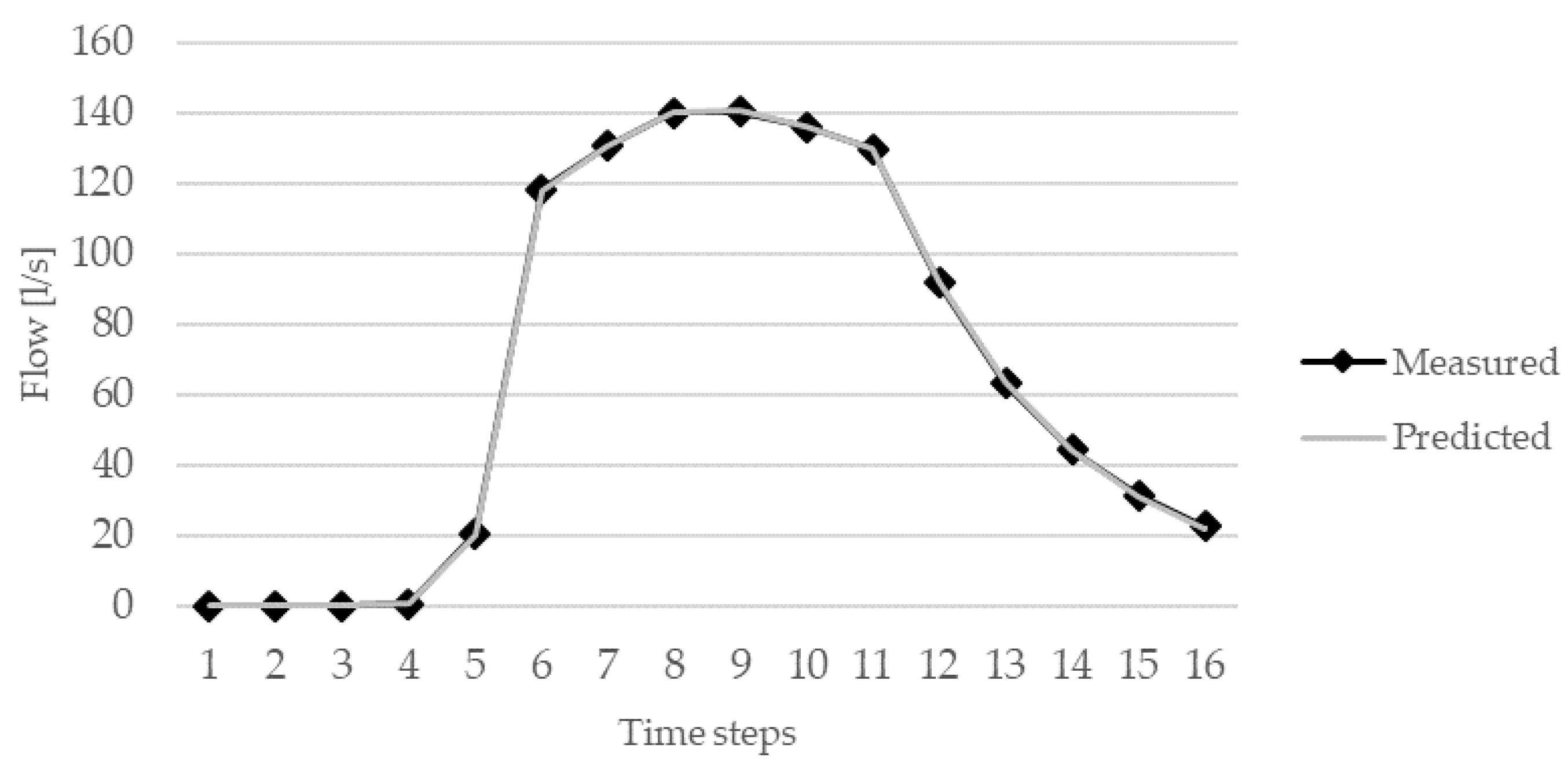
The second scenario was used to test the automatic calibration functionality and precision while calibrating infiltration parameters. In order to generate more runoff from the permeable surfaces, the rainfall intensity was increased compared to the previous scenario, and changed to 50 mm/h. The LMA function in the Excel add-in was used because it enables simultaneous calibration of more than two parameters. Three parameters from the Horton infiltration model were selected: Max. Infil. Rate, Min. Infil. Rate and Decay Constant. Initial model results (indicated as “Measured”) to compare the precision and performance of the automatic calibration module were obtained with corresponding parameter values of Max Infil. Rate = 20, Min. Infil. Rate = 1 and Decay Constant = 3. The LMA automatic calibration module resulted in a minimal OF value of 1.21 with a concurrent maximal infiltration rate of 20.57, minimal infiltration rate of 1.76 and decay constant of 3.4. In this case, the initial values were 30, 2 and 5. The coefficient for calculation of the minimal step was 0.001. Maximal deviation between the initial model and the calibrated model flow rates at the outlet was 4.3%. The comparison of the artificially created measured data and predicted flow rate are presented in Figure 6. The results are in good agreement with earlier studies on SWMM calibration including catchments with permeable surfaces. For example, Rosa et al. [17] concluded that the model calibration was successful, because the difference between the weekly observed and modelled runoff volumes was up to 12%.
Additional tests were conducted to analyze the overall performance of the developed software, e.g., both trial-and-error and LMA approaches were used to find the catchments’ percentage of impervious area (defined as parameter ID3 in the Excel workbook). The initial simulation model was executed under the condition that the percentage of impervious area for the catchments was set to 50%. The trial-and-error approach with the initial maximal and minimal values of 100% and 0% found the solution ID3 = 50% with OF = 0. In the case of LMA, it was found that the limit values could be used as initial values. For example, in the aforementioned case, the LMA with the initial value of ID3 = 100% resulted in an error of the function not depending on the parameters. The initial value of ID3 = 70% provided a solution of ID3 = 50.02 with OF = 0.7.
Similar errors were observed in the case where the subarea routing was set from impervious area to pervious (or vice versa), and then to the drainage system through the inflow manhole. The developed automatic calibration module did not correctly calculate the flow routing in the case when the impervious percentage of the subarea was 100% or 0%. Under these conditions, water cannot flow from an area with 100% to an area with 0%. SWMM5 checks such constraints when it reads the input file and routes the water automatically to the inflow manhole. The current DLL version does not automatically change the input file in order to decrease the computation time for calibration. The user of the program has to double check the input file and make sure that the flow routing through the catchments subareas is defined correctly.
4. Conclusions
An automatic calibration module that uses two different optimization methods to find the suitable parameter values for the UDS model to fit the calculated results to measurements was created and tested. The module enables searching for the values of pre-determined calibration variables without the need for user intervention. This is a clear advantage compared to manual calibration procedures where the user typically runs a series of simulations and compares the results to determine the best values for the variables. The procedure for utilizing the developed module was outlined. Twelve new parameters were included in the calibration module to widen the calibration options of SWMM5 models significantly. Sensitivity analysis and testing of the DLL functions showed that the optimization software Minpack may be used for SWMM5 model calibration if the minimal step for the gradient methods is optimal. This reduces the calibration time significantly compared to other popular optimization methods like GA. The user interface of the calibration module was based on the MS Excel software that does not require expert knowledge in IT and software development. The set-up of the files and calibration is straightforward and procedures easily replicable.
Two scenarios were set up to analyze the performance of the developed automatic calibration module. In the first case, the subcatchments were defined as impervious to test the module’s functionality when calibrating Manning’s roughness and depth of depression storage on impervious areas. In the second case, the subcatchments were defined as pervious to test the module performance taking into account infiltration. In both scenarios the maximum deviation between the “measured” and predicted flow rates was less than 5% indicating that the model calibration was successful.
Additional tests were carried out to analyze the overall performance of the optimization tools and constraints of the calibration module. It was concluded that in the case of LMA, it is not recommended to set initial values for parameters that are equal to the parameter limits. In addition, it was found that flow routing inside a catchment area, i.e., determining whether flow is routed from pervious to impervious or directly to the inlet, has to be correctly defined prior to calibration, and faulty routings create errors.
The functionality tests of the developed tool confirmed that it can be used to automate the calibration of hydraulic models. Future work includes expanding the developed calibration module and testing the module in calibration of different urban drainage models. The user interface will be further designed to improve the users’ experience. A dedicated help file will be created to assist the usage of the tool for the experts in the field. The automated calibration module is available for testing for free on request.
Author Contributions
Conceptualization, I.A., A.V. and N.K.; methodology, I.A. and A.V.; software development, A.V.; validation, K.K. and N.K.; writing—original draft preparation, I.A. and A.V.; writing—review and editing, I.A., A.V., N.K. and K.K.; visualization, K.K. All authors have read and agreed to the published version of the manuscript.
Funding
This work was supported by the Estonian Research Council, grant number PRG667, and European Union (European Regional Development Fund) Interreg Baltic Sea Region Programme, grant number #R093.
Institutional Review Board Statement
Not applicable.
Informed Consent Statement
Not applicable.
Data Availability Statement
The data presented in this study are available on request from the corresponding author. The data are not publicly available due to the presented calibration module is at the moment available only on request.
Acknowledgments
Technical support of Murel Truu is greatly appreciated.
Conflicts of Interest
The authors declare no conflict of interest. The funders had no role in the design of the study; in the collection, analyses, or interpretation of data; in the writing of the manuscript, or in the decision to publish the results.
References
- Langeveld, J.G.; Schilperoort, R.P.S.; Weijers, S.R. Climate Change and Urban Wastewater Infrastructure: There Is More to Explore. J. Hydrol. 2013, 476, 112–119. [Google Scholar] [CrossRef]
- Alfieri, L.; Feyen, L.; Dottori, F.; Bianchi, A. Ensemble Flood Risk Assessment in Europe under High End Climate Scenarios. Glob. Environ. Chang. 2015, 35, 199–212. [Google Scholar] [CrossRef]
- Tapia, C.; Abajo, B.; Feliu, E.; Mendizabal, M.; Martinez, J.A.; Fernández, J.G.; Laburu, T.; Lejarazu, A. Profiling Urban Vulnerabilities to Climate Change: An Indicator-Based Vulnerability Assessment for European Cities. Ecol. Indic. 2017, 78, 142–155. [Google Scholar] [CrossRef]
- Saraswat, C.; Kumar, P.; Mishra, B.K. Assessment of Stormwater Runoff Management Practices and Governance under Climate Change and Urbanization: An Analysis of Bangkok, Hanoi and Tokyo. Environ. Sci. Policy 2016, 64, 101–117. [Google Scholar] [CrossRef]
- Mikovits, C.; Rauch, W.; Kleidorfer, M. Importance of Scenario Analysis in Urban Development for Urban Water Infrastructure Planning and Management. Comput. Environ. Urban 2018, 68, 9–16. [Google Scholar] [CrossRef]
- Beeneken, T.; Erbe, V.; Messmer, A.; Reder, C.; Rohlfing, R.; Scheer, M.; Schuetze, M.; Schumacher, B.; Weilandt, M.; Weyand, M. Real Time Control (RTC) of Urban Drainage Systems—A Discussion of the Additional Efforts Compared to Conventionally Operated Systems. Urban Water J. 2013, 10, 293–299. [Google Scholar] [CrossRef]
- Emmanuel, I.; Andrieu, H.; Leblois, E.; Janey, N.; Payrastre, O. Influence of Rainfall Spatial Variability on Rainfall–Runoff Modelling: Benefit of a Simulation Approach? J. Hydrol. 2015, 531, 337–348. [Google Scholar] [CrossRef]
- Salvadore, E.; Bronders, J.; Batelaan, O. Hydrological Modelling of Urbanized Catchments: A Review and Future Directions. J. Hydrol. 2015, 529, 62–81. [Google Scholar] [CrossRef]
- Teng, J.; Jakeman, A.J.; Vaze, J.; Croke, B.F.W.; Dutta, D.; Kim, S. Flood Inundation Modelling: A Review of Methods, Recent Advances and Uncertainty Analysis. Environ. Modell. Softw. 2017, 90, 201–216. [Google Scholar] [CrossRef]
- Behrouz, M.S.; Zhu, Z.; Matott, L.S.; Rabideau, A.J. A New Tool for Automatic Calibration of the Storm Water Management Model (SWMM). J. Hydrol. 2020, 581, 124436. [Google Scholar] [CrossRef]
- Cooper, V.A.; Nguyen, V.-T.-V.; Nicell, J.A. Calibration of Conceptual Rainfall–Runoff Models Using Global Optimisation Methods with Hydrologic Process-Based Parameter Constraints. J. Hydrol. 2007, 334, 455–466. [Google Scholar] [CrossRef]
- Sangal, S.K.; Bonema, S.R. A Methodology for Calibrating SWMM Models. J. Water Manag. Model. 1994, 2, 375–387. [Google Scholar] [CrossRef] [Green Version]
- Behrouz, M.S. Automatic Calibration of Storm Water Management Model (SWMM) with Multi-Objective Optimization; University at Buffalo: New York, NY, USA, 2018. [Google Scholar]
- Jin, X.; Jiang, Y.; Wu, W.; Jin, J. Automatic Calibration of SWMM Model with Adaptive Genetic Algorithm. In Proceedings of the 2011 International Symposium on Water Resource and Environmental Protection (ISWREP), Xi’an, China, 20–22 May 2011; pp. 891–895. [Google Scholar]
- Swathi, V.; Raju, K.S.; Varma, M.R.R.; Veena, S.S. Automatic Calibration of SWMM Using NSGA-III and the Effects of Delineation Scale on an Urban Catchment. J. Hydroinf. 2019, 21, 781–797. [Google Scholar] [CrossRef]
- Barco, J.; Wong, K.M.; Stenstrom, M.K. Automatic Calibration of the U.S. EPA SWMM Model for a Large Urban Catchment. J. Hydraul. Eng. 2008, 134, 466–474. [Google Scholar] [CrossRef]
- Rosa, D.J.; Clausen, J.C.; Dietz, M.E. Calibration and Verification of SWMM for Low Impact Development. J. Am. Water Resour. Assoc. 2015, 51, 746–757. [Google Scholar] [CrossRef]
- Kim, B.; Sanders, B.F.; Han, K.; Kim, Y.; Famiglietti, J.S. Calibration of Stormwater Management Model Using Flood Extent Data. Proc. Inst. Civil Eng. Water Manag. 2014, 167, 17–29. [Google Scholar] [CrossRef] [Green Version]
- Cristina, M.; Paule-Mercado, A.; Lee, C.-H. Calibration of the SWMM for a Mixed Land Use Catchment in Yongin, South Korea. Desalin. Water Treat. 2017, 63, 381–388. [Google Scholar] [CrossRef]
- Del Giudice, G.; Padulano, R. Sensitivity Analysis and Calibration of a Rainfall-Runoff Model with the Combined Use of EPA-SWMM and Genetic Algorithm. Acta Geophys. 2016, 64, 1755–1778. [Google Scholar] [CrossRef] [Green Version]
- Shinma, T.A.; Reis, L.F.R. Incorporating Multi-Event and Multi-Site Data in the Calibration of SWMM. Procedia Eng. 2014, 70, 75–84. [Google Scholar] [CrossRef] [Green Version]
- Savić, D.A.; Bicik, J.; Morley, M.S. A DSS Generator for Multiobjective Optimisation of Spreadsheet-Based Models. Environ. Modell. Softw. 2011, 26, 551–561. [Google Scholar] [CrossRef] [Green Version]
- Goldberg, D.E.; Holland, J.H. Genetic Algorithms and Machine Learning. Mach. Learn. 1988, 3, 95–99. [Google Scholar] [CrossRef]
- Vassiljev, A.; Koppel, T. Estimation of Real-Time Demands on the Basis of Pressure Measurements by Different Optimization Methods. Adv. Eng. Softw. 2015, 80, 67–71. [Google Scholar] [CrossRef]
- Levenberg, K. A Method for the Solution of Certain Non-Linear Problems in Least Squares. Q. Appl. Math. 1944, 2, 164–168. [Google Scholar] [CrossRef] [Green Version]
- Marquardt, D.W. An Algorithm for Least-Squares Estimation of Nonlinear Parameters. J. Soc. Ind. Appl. Math. 1963, 11, 431–441. [Google Scholar] [CrossRef]
- Rossman, L.A. Storm Water Management Model User’s Manual Version 5.1; EPA: Cincinnati, OH, USA, 2015.
- Niazi, M.; Nietch, C.; Maghrebi, M.; Jackson, N.; Bennett, B.R.; Tryby, M.; Massoudieh, A. Storm Water Management Model: Performance Review and Gap Analysis. J. Sustain. Water Built. Environ. 2017, 3, 04017002. [Google Scholar] [CrossRef] [Green Version]
- SWMM-Docs: Open Water Analytics Stormwater Management Model. Available online: http://wateranalytics.org/Stormwater-Management-Model/index.html (accessed on 16 March 2021).
- Dent, S.; Hanna, R.B.; Wright, L.T. Automated Calibration Using Optimization Techniques with SWMM RUNOFF. J. Water Manag. Model. 2004, 12, 385–408. [Google Scholar] [CrossRef] [Green Version]
- Koppel, T.; Vassiljev, A. Calibration of a Model of an Operational Water Distribution System Containing Pipes of Different Age. Adv. Eng. Softw. 2009, 40, 659–664. [Google Scholar] [CrossRef]
- Dennis, J.E., Jr.; Schnabel, R.B. Numerical Methods for Unconstrained Optimization and Nonlinear Equations; Classics in Applied Mathematics; SIAM—Society for Industrial and Applied Mathematics: Philadelphia, PA, USA, 1996; ISBN 978-0-89871-364-0. [Google Scholar]
- Hamming, R.W. Numerical Methods for Scientists and Engineers, 2nd ed.; Dover Publications: Mineola, NY, USA, 1973; ISBN 978-0-486-65241-2. [Google Scholar]
- Gill, P.E.; Murray, W.; Wright, M.H. Practical Optimization; Academic Press: Cambridge, MA, USA, 1981; ISBN 0-12-283950-1. [Google Scholar]
- Moré, J.J.; Garbow, B.S.; Hillstrom, E. User Guide for MINPACK-1; Argonne National Laboratory: Argonne, IL, USA, 1980. [Google Scholar]
- Warsta, L.; Niemi, T.J.; Taka, M.; Krebs, G.; Haahti, K.; Koivusalo, H.; Kokkonen, T. Development and Application of an Automated Subcatchment Generator for SWMM Using Open Data. Urban Water J. 2017, 14, 954–963. [Google Scholar] [CrossRef]
Figure 1.
Flowchart of the developed calibration module.

Figure 2.
An example of the OF shape for: (a) small step in Manning’s roughness coefficient change; (b) a large step in Manning’s roughness coefficient change.
Figure 2.
An example of the OF shape for: (a) small step in Manning’s roughness coefficient change; (b) a large step in Manning’s roughness coefficient change.

Figure 3.
User interface in Excel for the LMA approach.

Figure 4.
User interface in Excel for the calibration results.

Figure 5.
Layout of the UDS network used to test the functioning of the calibration module.

Figure 6.
Comparison of the measured and predicted flow rates for Scenario 2.


Table 1.
List of the parameters recommended to be included in calibration by [12].
Table 1.
List of the parameters recommended to be included in calibration by [12].
| 1. Percentage of impervious areas |
| 2. Depression storage for impervious and pervious areas |
| 3. Subcatchment widths, Manning’s roughness coefficients for overland and sewer flow, and ground slopes |
| 4. The initial and final soil infiltration capacities |
Table 2.
List of parameters recommended to be included in the calibration in case of high groundwater levels [30].
Table 2.
List of parameters recommended to be included in the calibration in case of high groundwater levels [30].
| 5. Elevation of initial water table stage |
| 6. Threshold stage for groundwater flow |
| 7. Channel water influence factor |
| 8. Groundwater flow coefficient |
| 9. Groundwater flow exponent |
| 10. Coefficient for channel water influence |
| 11. Exponent for channel water influence |
Table 3.
Set functions for the automatic calibration module developed in the present study.
| Parameter | Included in OWA Toolkit | Added by the Authors |
|---|---|---|
| Links | ||
| Pipe roughness | X | |
| Subcatchment | ||
| Impervious percent | X | |
| Manning’s roughness for impervious area | X | |
| Manning’s roughness for pervious area | X | |
| Depression storage for impervious area | X | |
| Depression storage for pervious area | X | |
| Subcatchment width | X | |
| Subcatchment slope | X | |
| Subcatchment area | X | |
| Green-Ampt infiltration method | ||
| Suction head | X | |
| Hydraulic conductivity | X | |
| Initial deficit | X | |
| Horton infiltration method | ||
| Maximal infiltration rate | X | |
| Minimal infiltration rate | X | |
| Decay constant | X |
Table 4.
Comparison of LMA and trial-and-error-based calibration results for the first scenario.
| Surface 21 × 21 First Try | Surface 21 × 21 s Try | Levenberg-Marquard | ||||||
|---|---|---|---|---|---|---|---|---|
| Measured Flow Rate, l/s | Predicted Flow Rate, l/s | Square of Difference | Measured Flow Rate, l/s | Predicted Flow Rate, l/s | Square of Difference | Measured Flow Rate, l/s | Predicted Flow Rate, l/s | Square of Difference |
| 0.000 | 0.000 | 0.000 | 0.000 | 0.000 | 0.000 | 0.000 | 0.000 | 0.000 |
| 10.049 | 10.263 | 0.046 | 10.049 | 10.049 | 0.000 | 10.049 | 10.002 | 0.002 |
| 258.343 | 258.794 | 0.204 | 258.343 | 258.343 | 0.000 | 258.343 | 258.372 | 0.001 |
| 558.113 | 559.231 | 1.250 | 558.113 | 558.113 | 0.000 | 558.113 | 558.424 | 0.097 |
| 659.372 | 656.667 | 7.317 | 659.372 | 659.372 | 0.000 | 659.372 | 659.701 | 0.108 |
| 457.501 | 458.727 | 1.502 | 457.501 | 457.488 | 0.000 | 457.501 | 457.541 | 0.002 |
| 401.715 | 404.901 | 10.152 | 401.715 | 401.720 | 0.000 | 401.715 | 401.790 | 0.006 |
| 351.406 | 353.999 | 6.720 | 351.406 | 351.400 | 0.000 | 351.406 | 351.765 | 0.129 |
| 308.297 | 311.940 | 13.271 | 308.297 | 308.282 | 0.000 | 308.297 | 308.199 | 0.010 |
| 266.599 | 269.697 | 9.597 | 266.599 | 266.463 | 0.019 | 266.599 | 266.455 | 0.021 |
| 237.637 | 241.445 | 14.501 | 237.637 | 237.644 | 0.000 | 237.637 | 237.586 | 0.003 |
| 132.305 | 135.597 | 10.839 | 132.305 | 132.305 | 0.000 | 132.305 | 132.409 | 0.011 |
| 81.562 | 84.098 | 6.433 | 81.562 | 81.562 | 0.000 | 81.562 | 81.686 | 0.016 |
| 54.479 | 56.389 | 3.648 | 54.479 | 54.479 | 0.000 | 54.479 | 54.592 | 0.013 |
| 38.397 | 39.943 | 2.391 | 38.397 | 38.397 | 0.000 | 38.397 | 38.496 | 0.010 |
| 28.212 | 29.419 | 1.458 | 28.212 | 28.212 | 0.000 | 28.212 | 28.295 | 0.007 |
| Objective function OF | 89.329 | 0.019 | 0.433 | |||||
Publisher’s Note: MDPI stays neutral with regard to jurisdictional claims in published maps and institutional affiliations. |
© 2021 by the authors. Licensee MDPI, Basel, Switzerland. This article is an open access article distributed under the terms and conditions of the Creative Commons Attribution (CC BY) license (https://creativecommons.org/licenses/by/4.0/).
Share and Cite
MDPI and ACS Style
Annus, I.; Vassiljev, A.; Kändler, N.; Kaur, K. Automatic Calibration Module for an Urban Drainage System Model. Water 2021, 13, 1419. https://doi.org/10.3390/w13101419
AMA Style
Annus I, Vassiljev A, Kändler N, Kaur K. Automatic Calibration Module for an Urban Drainage System Model. Water. 2021; 13(10):1419. https://doi.org/10.3390/w13101419
Chicago/Turabian StyleAnnus, Ivar, Anatoli Vassiljev, Nils Kändler, and Katrin Kaur. 2021. "Automatic Calibration Module for an Urban Drainage System Model" Water 13, no. 10: 1419. https://doi.org/10.3390/w13101419
Note that from the first issue of 2016, this journal uses article numbers instead of page numbers. See further details here.