Assessing Water Withdrawals in Scarce-Data Transboundary Areas by Use of Dynamic Precipitation–Flow Relationships: The Case of the Hasbani River Basin

Abstract

The present study proposes a nonstandard solution to the problem of assessing water withdrawals (AWW) in the scarce-data transboundary basin. The applied AWW method operates with the open-source available data on precipitation and river flow and thereby overcomes the usual restriction due to lack of data on shared water use in the Middle East. Analysis of dynamic precipitation-flow relationships enable to separate the effect of water withdrawals from the total decline of river flow under the decreasing precipitation. This study is the first which provides complete information (1972–2020) on water withdrawals from total, surface, and base flow of the Hasbani River (Lebanon). The resulting values that exceed by far earlier published estimates were confirmed by (i) indirect indices (area of irrigated land and population), and (ii) validation of the AWW method based on independent data on water use (Israel Water Authority). The study results are useful for water balance estimations, as well as for management of water resources in the Jordan River headwaters basin and in the entire Lake Kinneret Basin. The AWW method can be applied to other transboundary basins and enables historical and real-time monitoring of water withdrawals as a necessary database for settlement of riparian water relations.

1. Introduction

In the Middle East, most of the river flow originates outside the countries, and transboundary waters represent over two-thirds of the overall region water resources [1,2]. In a transboundary basin, no riparian state can independently dispose of its water, and all countries are compelled to consider each other’s water rights and demands. Under grave shortage of water resources and uncertainty of regular water supply, such situation inevitably causes tension and discord in riparian water relations. It also implies the need for agreements and cooperation on water issues despite seemingly insurmountable geopolitical, socio-economic, and management problems and the negative historical experience of such efforts. It is evident that absence of the complete picture of water-related dynamics in transboundary basins and the lack of a basin-wide vision over the shared waters may result in disputes among the riparian states and ultimately in an unsustainable and biased use of the resources. There is no doubt on the importance and need of reliable data for making water-use decisions, but unfortunately reality is different. The following examples (randomly selected from many similar ones) illustrate the real situation: “The absence of official data (from Syria) on the amount of water diverted from the Yarmouk has left much room for speculation over the years” [1], or “The water balance scheme in the Jordan River Basin is based on the available data to date, which were provided from the different sources and not believed to be so accurate or highly consistent” [3], etc.

Such situations are due to strained international relations between the riparian states in the transboundary basin caused by internal economic, political, and national interests. All this may result in secrecy and even distortion of the data on water use [4,5,6,7]. However, in many known cases (see below in the present paper), the situation was aggravated not only and not so much by the availability (or secrecy) of data but because of the real lack or absence of data. Both of these circumstances determine and confirm the relevance of the proposed study topic which is assessing water withdrawals in the transboundary basin by using alternative data on precipitation and river flow.

The studied Hasbani River (named Snir in Israel) is one of the major tributaries of the Upper Jordan River (UJR) which contributes more than a quarter of the total inflow to it (Figure 1). The catchment area of the transboundary Hasbani basin is shared between Lebanon and Israel at respective rates of 97% and 3%. Hence, most of the flow formation and water use occur in the Lebanese part of the basin. The present study revealed significant decrease (about 50%) of the Hasbani River annual flow during 1940–2017 and only 13–15% decrease of the annual precipitation gauged in this period at the representative stations. Such significant flow decline of the Hasbani River cannot be caused only by the precipitation decrease but seems to be also the result of the developing water use.

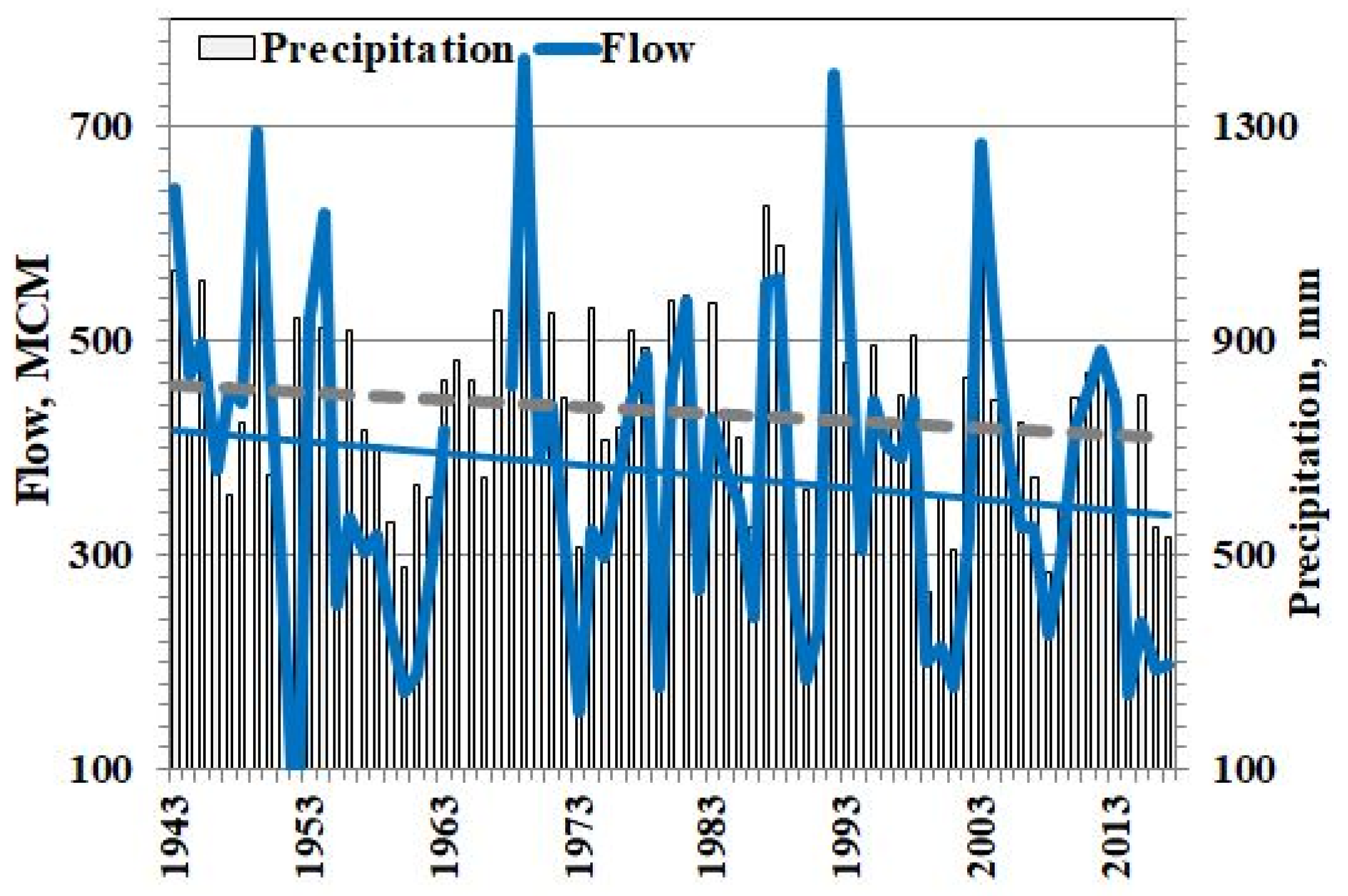
A drastic decrease in the flow of rivers in Lebanon has been recorded during the last three decades [8]. Decreases of spring and stream flow were documented both in the Jordan River basin [9,10,11], as well as in the Litani basin in Lebanon [12]. Data on available water (AW) in Lake Kinneret (1975–2007) indicated a decreasing trend which was concurrent with the decreasing trend in precipitation and the increasing water use in the entire Lake watershed. According to the Israeli Water Authority, the increasing water use explains at least three quarters of the total decrease in the AW during this period [10,13]. Concurrently, statistical analyses of rainfall time series in Israel have not detected significant decrease in rainfall trends [14,15].

There is no major disagreement that both climate change and increasing human activity impact the water balance of the Jordan River headwaters and of the entire Lake Kinneret Basin. However, the relative contribution of each factor remains to be debated especially considering the unspecified Lebanese water use from the Hasbani River [9,13,16,17,18,19]. The published values of the Hasbani water use by Lebanon are rather uncertain and insignificant (see Section 6.1 below). The question remains open whether these estimated values are sufficient to explain the significant decrease in the flow of the Hasbani River (1940–2017), even taking into account the observed decrease in precipitation.

Due to insufficient data on water use in the Hasbani River basin, it is evident that (i) any clarification and updating of these data would be an essential contribution to assessing the water balance in the UJR basin, and (ii) the problem requires an alternative approach and a nonstandard solution allowing to differentiate climate and human impacts on the river flow regime. For this purpose the present study applies the method proposed by the authors [20] for assessing water consumption in a transboundary basin under conditions of scarce available data on water use. The method is based on analyzing the alternative data on precipitation and river flow and was efficiently applied to the Yarmouk River (1971–2009) up to the Maqaren Station (Syrian part of the basin). In the present paper, the method was conceptually revised taking into consideration the outcomes of recent widespread discussions of the difference between “water consumption” and “water supply” (use, withdrawal, abstraction). By definitions of the USGS Glossary [21], the object of this study is accepted as assessing water withdrawals, but not water consumption (as in the previous publication [20]). The title of the present article has been updated accordingly. Nevertheless, the calculation technique remained unchanged. Therefore, withdrawals are estimated as the total amount of water removed from the source (or did not reach the downstream hydrometric station and not included in the gauged flow), regardless of how much of that total is consumptively (or non-consumptively) used [22]. The designation AWW (assessing water withdrawals) of the method is hereinafter used.

Assessing the impact of water use on water resources is one of the urgent problems of modern hydrology. The publications offer a huge number of approaches, methods, and models for its solution in general and for particular cases. These studies apply nonparametric methods to analyze the changing point and annual trend in various hydro-meteorological time series (e.g., rainfall, temperature, flow and groundwater levels), and afterwards, they employ an integrated model of surface-groundwater flow to simulate effects of alternative water-use scenarios on groundwater levels and streamflow. The differences are in kind and scale of the model, research goal, and results. Some typical examples of similar studies are presented in Appendix A.

In contrast to the modeling flow with consideration of water use as an influencing driver (in the studies presented above), the AWW method offers an inverse solution to the problem. The latter assesses water withdrawal using data on the basin input and output (measured precipitation and flow) within the simple statistical model. This is the novelty of the method and its specificity.

The main objective of the present study can be formulated as (i) Assessing water withdrawals from the Hasbani river flow (Lebanon) by the AWW method; (ii) validation of the AWW method and confirmation of reliability of the obtained results.

The paper is built as following: Section 2 presents a brief description of the study area; Section 3 presents the available data and introduces the AWW method which is adopted for the case study in Section 4; Section 5 presents a wide range of results such as estimated withdrawals from the Hasbani River for the study period, validation of the AWW method, confirmation of estimates by indirect indices, and estimated withdrawals from surface and base flow; in Section 6 results obtained are discussed; conclusions and recommendations are provided in Section 7.

It is important to emphasize that the use of the Hasbani river flow in Lebanon has been for decades a source of tension and of discord between Lebanon and Israel. To the present day there is no agreement on the use of these transboundary waters. The proposed study focuses on hydrological aspects of the problem (specifically, on assessing water withdrawals from the Hasbani River by alternative hydrometric and precipitation data), disregarding geopolitical, socio-economic, and management issues, and without touching upon the issue of transboundary water relations and disagreement between both riparian countries.

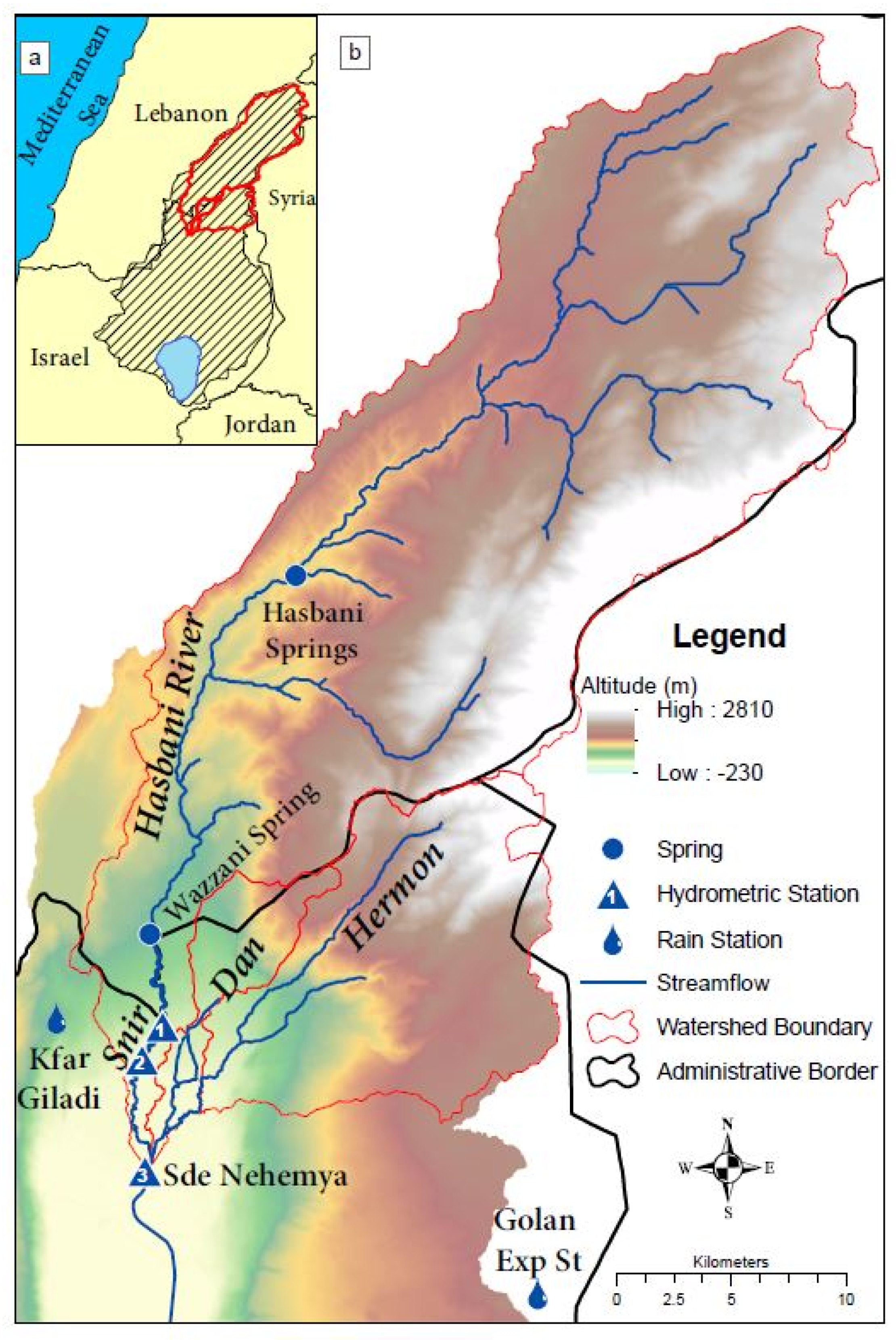
2. Study Area

The Hasbani (Snir) River is one of the major tributaries of the Upper Jordan River (UJR) (Figure 1). It is a significant flow source, which contributes 26% of the total inflow to UJR while the remaining flow is formed by the Dan and Hermon Rivers [10,16,17]. In the present study, contribution of the Hasbani River updated to 30%.

The main sources of the Jordan River are located in the southern foothills of the Hermon Range, which is an elongated anticline, mostly built of >2000 m Jurassic karstic limestone. The Mt. Hermon range is 55 km long and 25 km wide. Its high regions (above 1000 m a.s.l., the summit 2814 m a.s.l.) receive the highest annual precipitation (>1400 mm/year).

The Hasbani River originates from the Hasbani springs (outflowing from karst in the northern part of the basin), flows southwards for about 20 km until reaching the point at which its flow is substantially increased by the Wazzani spring. About 0.5 km downstream the river reaches the Lebanese–Israeli border, flows for about 4 km along the border, and after 7 km joins with Hermon (Banias) and Dan Rivers in northern Israel near Sede Nehemya (Yosef Bridge), to form the Upper Jordan River. The surface catchment area of the transboundary Hasbani basin (614 sq. km) is shared between Lebanon and Israel as 97% and 3%, respectively. Most of the flow is formed and used in the Lebanese part of the basin.

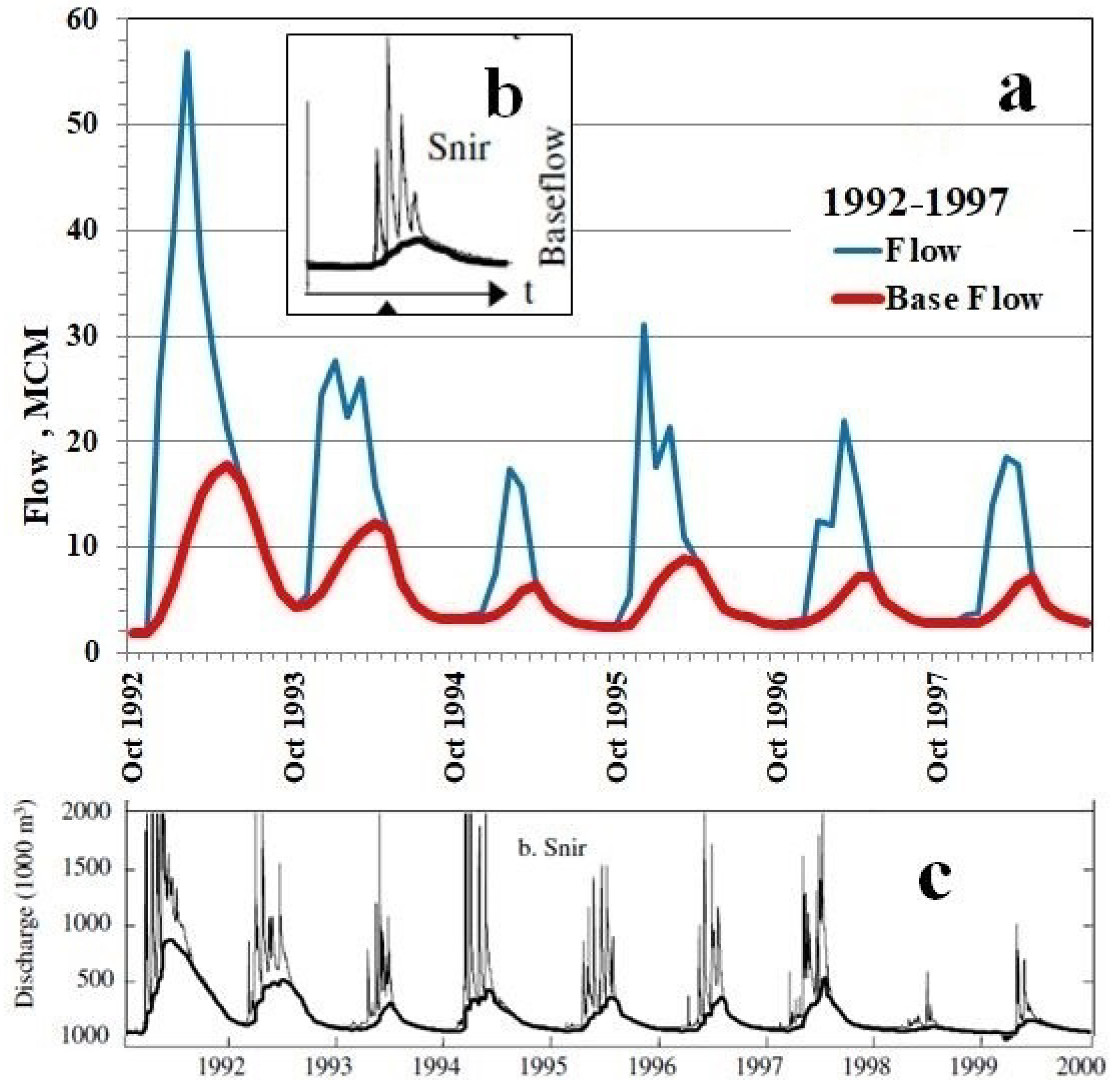
The climate in southern Lebanon is Mediterranean. Precipitation over the Hasbani Basin is characterized by a wet (rainy) season from October to April and by a dry hot season with relatively little to no precipitation from May to September. On Mount Hermon snow usually falls on the elevated areas from December to March, and persists on areas 1400–1900 m a.s.l. and above until March–June (depending on local conditions). The major replenishment of Hasbani River comes from precipitation, as well as from snowmelt and springs which are fed by groundwater from calcareous aquifers recharged by snow and rains. The Hasbani River derives most of its flow from the Wazzani and Hasbani karst springs (Lebanon) with the annual respective contribution of 45 and 30 MCM/y. The rest of the measured discharge is contributed by surface runoff of three tributaries and their seasonal rivulets or flow from other upstream springs. The contribution of the Wazzani spring is very important, since this is the only continuous year-round flow into the river. Water supplies to domestic and agricultural demands in the Hasbani Basin derive from springs, directly from the river and from public and private wells. In this section, origin of data is from [1,16,17,23,24,25,26,27,28].

3. Data and Method

3.1. Data

Due to lack of sufficient and reliable data on the use of water resources in the transboundary Hasbani river basin, the alternative data on precipitation and river flow was used within the Assessing Water Withdrawal (AWW) method. These data are the annual series of flow of the Hasbani River recorded at the Mayan Barukh and Dan Road Bridge hydrometric stations (1940–2020) and annual series of precipitation gauged at Kfar Giladi (1940–2020) and at Golan Experimental (1970–2020) stations (see map in Figure 1). Sources of data are the Israel Hydrological Service and the Israel Meteorological Service, respectively.

Expanding the study to include a separate assessment of withdrawals from surface and base flow required data on the monthly flow of the Hasbani River (1940–2020) recorded at the Mayan Barukh and Dan Road Bridge hydrometric stations (the Israel Hydrological Service).

It is important to notice that years 1940–2017 are taken as the study period, while series 2018–2020 are considered as independent data.

Validation of the AWW method required the following additional data: (i) annual series (1943–2017) of the Upper Jordan River flow recorded at Sede Nehemya Station (the Israel Hydrological Service) and (ii) data (1975–2014) supplied by the Israel Water Authority on water use in the Upper Catchments of the Jordan River (included the Dan and the Hermon basins in Israel but without the Hasbani basin in Lebanon (Figure 1)).

3.2. The AWW Method

The assessing water withdrawal (AWW) method focuses on the detection and attribution of the trends in historical time-series of flow and precipitation at the annual scale. According to [29], the term “Detection” implies that an observed change is significantly different (in a statistical sense) from what can be explained by natural internal variability. Hence, detection is primarily a statistical argument, without explaining the causes for change. The term “Attribution” is the process of establishing the most likely causes (drivers) for the detected change with defined levels of confidence.

At the stage of the trend detection, the AWW method tests the following hypotheses:

• The significant decrease of linear trend is detected in historical time-series of flow and precipitation while the precipitation trend is less and cannot completely explain the decrease of flow.
• Dependence between flow and precipitation (PF relationship) is observed in the study period.
• During subsequent sub-periods, the dynamic PF relationship demonstrates the consistent flow decline when for the same precipitation in the basin, less and less runoff was measured at the downstream station.

The next step is the flow trend attribution. If the first and the second hypotheses are confirmed significantly, then a decrease in precipitation (climate signal) can be considered as an obvious (but not the only) driving force behind a decrease in flow. Confirmation of the third hypothesis indicates the influence of additional driver which is similar to the increased water withdrawal. Most likely, this effect is associated with human activities (development of irrigation, economic and domestic needs, etc.), but the influence of increase in total evaporation due to global air warming and other possible reasons is not excluded. The attribution of flow mode changes to specific drivers is discussed in Section 6.2. Until then, we use the term “withdrawals” without detailed interpretation, assuming that withdrawals are the total amount of water removed from the river (or did not reach it) and are not included in the measured flow.

If the third hypothesis is confirmed, the ultimate goal of the study is to assess the influencing factor (water withdrawals) by comparison of the measured annual flow with its “natural” value. The latter is calculated by the PF relationship (natural curve) for the earlier (unregulated) period. Solution of this problem would be trivial if the historical flow data are available (like the Hasbani flow series from 1939/40 to 1970/71 in the present study). Otherwise, the task becomes more difficult. In such case, it is proposed to construct a “natural curve” using the available historical data, which unfortunately may be very limited in transboundary basins [19,20].

On the graph of precipitation–flow relationships (see following figures) the natural curve should be the upper envelope of the field of points. The deviation of the corresponding point (measured yearly flow) downward from the natural PF curve can be regarded as an estimate of the annual volume of withdrawals. However, considering the statistical nature of the PF relationship (due to influence of other unaccounted factors), the corresponding sub-period curve is proposed to be used in the calculation procedure instead of the corresponding point. By this way, the annual volume of withdrawals is estimated as a distance between the natural PF curve and the corresponding sub-period PF curve and as a function of the yearly precipitation:

W_j = Q_ntr(X_j) − Q^k(X_j)

(1)

where W is water withdrawals, Q_ntr is the natural flow, Q^k is flow calculated by the k-th dynamic PF relationship (in accordance with sub-period), X is precipitation, and j is the time step number (year).

Thus, the AWW method evaluates water withdrawals as a current shortage (deficit) of flow, which in an earlier “natural” period could have been formed by the same precipitation in the basin, but during the period under consideration it did not reach the gauging station downstream due to upper water use and other potential factors. This formulation is consistent with the interpretation of this term above.

It is important to emphasize that the AWW method enables to separate the influence of climatic precipitation changes on the flow from the anthropogenic impacts (and other potential drivers). In the process of computing water withdrawals (as purpose of the study), the precipitation change is implicitly taken into account by the method definition, because dynamics of the PF relationship (but not declined flow trend) are involved in analysis.

Finally it should be noted that precipitation–flow (PF) relationships are widely used in hydrological research for solving problems of water forecasts and water resources management, for assessing hydrological effects of the climate change, and for other purposes. In each case, the necessary initial step is to determine the PF relationship for its further use with a specific purpose. Wherein input scenarios and output results can be temporally varied, PF relationships are supposed to remain unchanged (e.g., [9,10]). Unlike this approach, the AWW method is based on the retroactive analysis of the dynamic PF relationship which may change primarily as a result of human activity in the basin.

The practical application of the AWW method is described in detail in the following Section 4. Particular attention should be given to Appendix B, which presents estimates of the statistical significance of all calculated trends (Mann–Kendall Test) and correlation coefficients (p-Value Test for Pearson R Score) in this study.

4. Application of the AWW Method to the Hasbani River

4.1. Adaptation to the Case-Study

There is a long and complete series of the Hasbani River flow measured at the Israel hydrometric stations (Mayan Barukh and Dan Road Bridge) since hydrological year 1939/40. The stations are located in close vicinity near the Lebanon-Israel border (Figure 1). For integrated series 1940-2017 (see Section 4.2), the mean annual flow of the Hasbani River was evaluated as 112 MCM/y but during successive 26-year sub-periods (1940–1965, 1966–1991 and 1992–2017) this value decreased respectively from 128 to 121 and 88 MCM/y. For the last sub-period the mean flow differs significantly from the previous two (p-value is less than 0.05) [30].

Figure 2 demonstrates the significant decrease (55%) of the Hasbani River annual flow during 1940–2017 and only 13% decrease of the annual precipitation recorded for this period at the representative Kfar Giladi station. By the Mann–Kendall Test (Appendix B,

Table A1. Mann–Kendall test of trend [76,77].

Station/Basin	Element	Period	Figure	Trend						Significance Level (alpha)	Test Result
				Formula	Unit	Start	End	Difference	Difference %
Kfar Giladi St.	Precipitation	1940–2017	Figure 2	y = −1.440x + 829.2	mm	828	717	−111	−13%	0.10	yes
Hasbani	Flow	1940–2017	Figure 2	y = −1.129x + 159.0	MCM	158	71	−87	−55%	0.05	yes
Hasbani	Withdrawals	1972–2020	Figure 6a	y = 0.5584x + 23.09	MCM	24	50	27	113%	0.05	yes
Hasbani	Flow	1972–2020	Figure 6a	y = −1.132x + 122.6	MCM	121	67	−54	−45%	0.05	yes
Kfar Giladi St.	Precipitation	1943–2017	Figure 8	y = −1.329x + 819.3	mm	818	720	−98	−12%	0.25	yes
Jordan–Sd. Neh.	Flow	1943–2017	Figure 8	y = −1.062x + 417.5	MCM	416	338	−79	−19%	0.15	yes
Hasbani	Withdrawals	1975–2014	Figure 9	y = 0.3296x + 27.75	MCM	28	41	13	46%	0.40	yes
UCJR (Israel)	Water Use	1975–2014	Figure 9	y = −0.6688x + 67.50	MCM	67	41	−26	−39%	0.05	yes
Jordan–Sd. Neh.	Flow	1975–2014	Figure 10	y = −0.6465x + 394.1	MCM	393	368	−25	−6%	>0.40	no
UCJR	Withdr. SUM	1975–2014	Figure 10	y = −0.3392x + 95.24	MCM	95	82	−13	−14%	>0.40	no
Hasbani	Surface Flow	1940–2020	Figure 14a	y = −0.5083x + 74.91	MCM	74	34	−41	−55%	0.05	yes
Hasbani	Base Flow	1940–2020	Figure 14a	y = −0.5955x + 83.43	MCM	83	35	−48	−58%	0.05	yes
Hasbani	SF Withdr.	1972–2020	Figure 16a	y = 0.1436x + 15.03	MCM	15	22	7	45%	0.40	yes
Hasbani	BF Withdr.	1972–2020	Figure 16a	y = 0.4148x + 8.057	MCM	8	28	20	235%	0.05	yes

Notes: Mann–Kendall trend test is a nonparametric test used to identify a trend in time series. Statistical analyses were executed in Real Statistics Resource Pack for Excel (Release 7.5.1).

), detected linear trends are statistically significant (with significance level alpha 0.05 and 0.10 for flow and precipitation, respectively). Comparison of trends indicates that the decrease of precipitation is insufficient to explain the considerable flow decline of the Hasbani River, and the flow change seems to be caused by the added drivers such as the developing water use or others.

For the above trend-analyses (Figure 2), precipitation data at the representative Kfar Giladi station was used (PF correlation coefficient 0.889). It should be noted that hereinafter (i) annual precipitation in the Hasbani Basin is presented as the value AVG Rain which is the average annual precipitation at Kfar Giladi and Golan Experimental representative gages (Figure 1), (ii) 78-years period 1940–2017 is taken in account (by recorded series at Kfar Giladi Station), and (iii) 30-years gap (1940–1969) in precipitation series of Golan Experimental Station was reconstructed by data of Kfar Giladi Station (with cross-correlation coefficient 0.940 for 1970–2017).

Prior to averaging (AVG Rain), the depths of annual precipitation at Kfar Giladi and Golan Experimental stations are z-score standardized, i.e., transformed to values with a mean of zero and a standard deviation of 1. The z-score standardized variable is the distance between data point and the sample mean in relation to the sample standard deviation. In application of statistics, variables measured on different scales or on a common scale with widely differing ranges are often adjusted by this way for comparison or averaging [31,32].

It is important to notice that according to the regionalization of the rainfall field in the Upper Jordan River (Lake Kinneret Basin) [33], the selected Kfar Giladi and Golan Experimental stations represent different regions: (R1) Upper Galilee and Western Hasbani Basin and (R3) Eastern Hasbani Basin, Northern Golan and Hermon, respectively. Here regions are named as in the referenced paper, in which the reginal division was done considering the specific relationships between the mean annual precipitation depth and elevation.

As a result, the present study operates with the quite long precipitation data series (1940–2017), and AVG Rain is a statistical characteristic of the precipitation field which is more representative and sustained (against random errors) in comparison with the point data. The efficiency of used approach is confirmed by statistics in

Table 1. Correlation coefficient between Hasbani River flow and different characteristics of precipitation.

Precipitation	Period	Correlation Coefficient
Kfar Giladi St.	1940–2017	0.889
Golan Exp. St.	1970–2017	0.940
AVG Rain	1970–2017	0.917
AVG Rain	1940–2017	0.909

.

The Hasbani River flow at Mayan Barukh Station in comparison with precipitation (as AVG Rain) during the study period (1940–2017) is presented in Figure 3.

4.2. Natural Flow Curve

The initial necessary step is to establish the Natural Flow Curve by analyses of PF relationship during the earlier unregulated period (1940–1971) considering the history of the hydrometric stations on the Hasbani River (see map in Figure 1). According to the Hydrological Year-Book of Israel [34], during 1940–1951 the Hasbani (Snir) flow was gauged at the Dan Road Bridge hydrometrical station. In 1952 a part of the Dan River water was diverted through the Qoren Channel into the Snir River upstream of the gauging station. Monthly and yearly flow figures for 1952–1962 represent measured values after deduction of the Qoren input. In 1963 the new Mayan Barukh station (with basin area reduction of less than 1%) started to work upstream of the existing Qoren and Dan Channels (the latter dug in 1962). However, due to technical difficulties in the operation of the new station, the previous downstream Dan Road Bridge Station continued to serve as supporting for flood measurements, and this situation persists to the present date. Since 1963 to the present time the Hydrological Year-Books of Israel [35] include data on the Snir (Hasbani) flow at both stations (with relevant comments), while the present study uses flow measured at the Mayan Barukh station.

Figure 4 reveals that during the initial (unregulated) period (1940–1971) there was a tight dependence between Snir (Hasbani) flow and precipitation. The uniformity of the PF relationship based on measurements at the Dan Road Bridge (1940–1951) and at Mayan Barukh (1963–1971) stations is noteworthy. The common relationship (for 1940–1971 period without 1952–1962 years) is accepted as the Natural Flow Curve of the Snir (Hasbani) River with the significant PF correlation coefficient 0.952 (Appendix B,

Table A2. p-value test for Pearson R score [78].

Station	Relationship	Period	Figure	Formula	R	N	p-Value	Test Result
Hasbani-Mayan Barukh	Natural Flow Curve	1940–1971 *	Figure 4	y = 2.681x2 + 55.66x + 130.0	0.952	21	<0.00001	Significant at p < 0.01
	Flow#AVG Rain	1972–2017	Figure 5a	y = 55.16x + 96.34	0.918	46	<0.00001
	Flow#AVG Rain	1972–1997	Figure 5b	y = 52.86x + 102.0	0.969	26	<0.00001
	Flow#AVG Rain	1998–2017 **	Figure 5b	y = 25.88x + 65.97	0.915	16	<0.00001
	Natural Flow Curve [2]	1972–2017	Figure 7	y = 3.795x2 + 56.79x + 127.2	0.974	46	<0.00001
Upper Jordan-Sede Nehemya	Natural Flow Curve [1]	1943–1955	Figure 11	y = 119.6x + 468.7	0.873	13	0.000098
	Flow#AVG Rain	1956–2017	Figure 11	y = 129.4x + 366.2	0.919	62	<0.00001
	Flow#AVG Rain	1943–2017	Figure 11 #	y = 129.6x + 384.8	0.881	75	<0.00001
	Natural Flow Curve [2]	1975–2014	Figure 12	y = 130.8x + 469.6	0.941	40	<0.00001
Hasbani-Mayan Barukh	Natural SF	1940–1971 *	Figure 15a	y = 1.124x2 + 33.70x + 60.58	0.915	32	<0.00001
	SF#AVG Rain (1)	1972–1997	Figure 15a	y = 32.69x + 44.68	0.969	26	<0.00001
	SF#AVG Rain (2)	1998–2017 **	Figure 15a	y = 18.77x + 32.15	0.913	20	<0.00001
	SF#AVG Rain	1972–2017	Figure 15a #	y = 33.72x + 45.40	0.933	46	<0.00001
	Natural BF	1940–1971 *	Figure 15b	y = 23.94x + 70.11	0.929	32	<0.00001
	BF#AVG Rain (1)	1972–1997	Figure 15b	y = 18.92x + 55.82	0.897	26	<0.00001
	BF#AVG Rain (2)	1998–2017 **	Figure 15b	y = 9.328x + 34.30	0.758	20	0.000108
	BF#AVG Rain	1972–2017	Figure 15b #	y = 21.42x + 50.94	0.860	46	<0.00001

Notes: * Period without 1952-1962; ** Period without 2003–2004, 2012–2013; # only points (without curve) are in the graph, R is correlation coefficient, N is number of years in series.

). Points (and curve 2) corresponding to measurements at the Dan Road Bridge (1952–1962) are placed mostly lower and were not taken into account. In all probability, this was due to above mentioned hydrometrical problems in this period connected with the inaccurate measurement of the water diversion from Dan to Snir.

4.3. Dynamic PF Relationship

Figure 5a demonstrates that the established Natural Flow Curve for the Snir (Hasbani) River is the upper envelope of the entire field of points related to the following 1972–2017 period. During this period there is a high accuracy dependence (with correlation coefficient 0.918) between flow and precipitation (flow rises as rainfall increases) while the curve is placed lower than the Natural Flow Curve and confirms the effect of the water withdrawals.

A comprehensive analysis of the relationship between precipitation and flow for 1972–2017 enabled to identify two specific sub-periods within this period (Figure 5b). The first sub-period of 26 years (1972–1997) stands out by the higher accuracy dependence of flow on precipitation (correlation coefficient 0.969) than during the whole period. In the following sub-period (1998–2017) the curve is placed lower and correlation coefficient (0.915) persists almost at the level of the overall PF relationship. All correlation coefficients are statistically significant (Appendix B, Table A2).

Further analysis showed that a more detailed presentation of the PF relationship is possible, but limited by the available data series and the statistical significance of the estimates.

Generally, during successive sub-periods (1972–1997 and 1998–2017) consistent flow decline is observed. This means that for the following sub-period, the same precipitation in the basin formed less flow (measured at the Mayan Barukh station) because of increasing water withdrawals.

The years 2003–2004 and 2012–2013 are exceptional because of the excessive annual flow as compared to the PF relationship for 1998–2017 sub-period. Detailed analysis did not show any natural cause for such sharp rise of the runoff coefficient which was observed both for surface and base flow too (see Section 5.4.2). On the other hand, the significant decrease of the river flow use (to the level of the initial unregulated period and of the previous sub-period, respectively) in these rainy years could be caused by the geopolitical and socio-economic (regional or local) factors. Though discussion of possible hypotheses is outside the scope of the present study, the authors consider it important (i) to show a possibility of such situation in transboundary basin and (ii) to raise this issue for a special research.

When the years 1940–1972 are used as the study period, the independent data deserve particular attention. These data are precipitation gauged at Kfar Giladi and Golan Experimental stations in years 2018–2020 and the Hasbani flow recorded at the Mayan Barukh station in these years. The respective points are located near the lower curve as continuation of the 1998–2017 sub-period (Figure 5b). It means that the independent data support the dynamic character of the PF relationship.

5. Results

5.1. Estimated Withdrawals from the Hasbani River

According to the AWW method, the natural PF curve (Figure 5b) serves as a basis for assessing the water withdrawals (1972–2017) in the Hasbani Basin (Lebanon). The annual volume of withdrawals is estimated by Equation (1) (in Section 3.2) as a distance between the natural PF curve and the corresponding sub-period PF curve, in accordance with the yearly precipitation. Independent 2018–2020 years are included in calculation by use of the 1998–2017 sub-period curve. For calculating the excepted 2003–2004 and 2012–2013 years, the natural curve and the 1972–1997 sub-period curve are respectively suggested.

Estimated withdrawals from the Hasbani River (Lebanon) vs. flow measured at Mayan Barukh Station (1972–2020) with detected linear trends are presented in Figure 6a. Natural flow of the Hasbani River as a sum of the measured flow and estimated water withdrawals (1972–2020) is presented in Figure 6b. Figure 6a demonstrates the significant decrease (45%) of the Hasbani River annual flow during 1972–2020 and sharper increase (113%) of the water withdrawals. By the Mann–Kendall Test, both detected linear trends are statistically significant (Appendix B, Table A1). Figure 6 demonstrates that against the background of decreased measured flow, increased withdrawals make more and more part of the natural flow.

Figure 7 presents the verification of the AWW method for the Hasbani River. This graph shows the relationship between the measured Hasbani flow and precipitation (1972–2017) in comparison with the different versions of the Natural Flow Curve being the upper envelope of the entire field of points related to this period. Every curve is a trend line of PF relationship based on the following flow data: (1)–measured flow in the unregulated period (1940–1971) (see Section 4.2), and (2)–sum of measured flow and calculated withdrawals (1972–2017) (see Figure 6b). It occurs that both versions of the Natural Flow Curve are very close. Their likeness serves as a verification of the AWW method by its definition.

Summing up,

Table 2. Summary of the Hasbani flow at Mayan Barukh Station and withdrawals from the Hasbani River (1972–2020).

Sub-Period	Measured Flow	Water Withdrawals
	MCM	MCM	%
1972–1983	113	30	21%
1984–1995	112	31	22%
1996–2007	88	38	30%
2008–2020	66	48	42%

Note to Table 2: Water withdrawals (%) is related to the natural flow (sum of measured flow and withdrawals).

presents the comparison of the mean annual values of the measured Hasbani flow and the calculated water withdrawals during successive 12(13) years sub-periods (1972–1983, 1984–1995, 1996–2007, and 2008–2020). These data indicate the following:

-

Measured flow was almost unchanged (112–113 MCM) during the two initial sub-periods but dropped sharply to 88 and 66 MCM in the third and the fourth sub-periods (decrease by 21% and 41%, respectively).

-

Contrarily, water withdrawals increased from 30–31 MCM during the two initial sub-periods to 38 and 48 MCM in the third and the fourth sub-periods (increase by 27% and 60%, respectively).

-

As a result, the portion of the water withdrawals within the natural flow doubled and reached 42% in 2008–2020.

5.2. Validation of the AWW Method

Until now, the AWW method has not been validated in any case of its application-neither for the Yarmouk Basin [20] nor for the Hasbani Basin (in the present paper). In both cases, this is due to a lack of independent and reasonably complete data on water use in the study basin. Such data (1975–2014) on water use in the Upper Catchments of the Jordan River (including the Dan and the Hermon basins in Israel but without the Hasbani basin in Lebanon) were supplied by the Israel Water Authority [36].

To apply this data it is necessary to expand the study area to the basin of the Upper Jordan River up to Sede Nehemya Station. This area (named the Upper Catchments of the Jordan River (UCJR)) includes watersheds of the major headwater sources—Hasbani (Snir), Dan and Hermon Rivers (see map in Figure 1). The area of the transboundary UCJR basin covers in total 860 sq. km which is shared (as 70% and 30%, respectively) by Lebanon (Hasbani basin) and Israel (other basins).

The mean annual flow of the Upper Jordan River at Sede Nehemya Station during 1943–2017 is evaluated (in the present study) as 382 MCM/y. However, for three 25-years sub-periods (1943–1967, 1968–1992, and 1993–2017) this value is reduced from 401 to 394 and 355 MCM/y, respectively.

Figure 8 demonstrates the apparent decrease (19%) in flow of the Upper Jordan River measured at the Sede Nehemya Station during hydrological years 1943–2017 and only 12% decrease in precipitation gauged during this period at the representative Kfar Giladi station. These data indicate that the precipitation decrease is insufficient to explain the flow decline of the Upper Jordan River. The previously estimated withdrawals from the Hasbani River in Lebanon and data on water use supplied by the Israel Water Authority corroborate the water use in the UCJR basin.

Figure 9 shows the water withdrawals in the Hasbani Basin (Lebanon) calculated by the AWW method vs. water use in the UCJR Basin (Israel) during 1975–2014 years. It is worth recalling that 30% of the total flow of the Upper Jordan River is formed in the Hasbani basin, while the remaining 70% is the contribution of the Dan and Hermon Rivers. The obvious (oppositely directed) linear trends were detected for both variables: the water withdrawals in the Hasbani Basin increased by 46% and water use in the UCJR Basin (Israel) decreased by 39%.

This is the first opportunity to compare water use in the Lebanese and Israeli parts of the UCJR Basin. As seen, until 1997 the water withdrawals in the Hasbani Basin varied from half to three quarters of the water use in the UCJR Basin (Israel). Further the water use in the Hasbani Basin increased and reached (and even exceed) the Israel water use, particularly considering the reduction of the latter following the drought in 1999–2000 (by the operative decision of the Israel Water Authority). In 2012–2014, water withdrawals in Lebanon decreased in contrast to its growth in Israel.

Summary for 10-years sub-periods is presented in

Table 3. Water withdrawals in the Hasbani Basin and water use in UCJR (Israel).

Sub-Periods	[Calc Hasbani]		[UCJR (Israel)]		[SUM]	Ratio
	MCM	%~SUM	MCM	%~SUM	MCM
1975–1984	30	33%	62	67%	92	0.47
1985–1994	31	36%	57	64%	88	0.55
1995–2004	32	37%	54	63%	86	0.53
2005–2014	45	52%	42	48%	86	0.74

Notes to Table 3: [Calc Hasbani] is the calculated withdrawals in the Hasbani Basin (Lebanon); [UCJR (Israel)] is water use at the Israeli part of UCJR Basin (by the Israel Water Authority); [SUM] is the total water use in UCJR as sum of [Calc Hasbani] and [UCJR (Israel)]; Ratio is [Calc Hasbani] related to [UCJR (Israel)].

. As seen, during four sub-periods the Hasbani withdrawals increased from 30 to 45 MCM (one-third to half of the total SUM). The opposite situation was observed for water use in UCJR (Israel): it dropped and in 2005–2014 approached the Hasbani withdrawals. Ratio between these components was up from 0.47 to 0.74.

The main conclusion from Figure 9 and Table 3 is the availability of data on water use in the UCJR Basin shared between Lebanon and Israel (1975–2014): calculated (by the AWW method) values for Hasbani Basin and independent data of the Israel Water Authority for the remaining basin area. The total water use (SUM) was compared with measured flow of the Upper Jordan River at Sede Nehemya Station (Figure 10). Insignificant negative trends are detected for both variables during 1975–2014.

In order to validate the AWW method, the present study proposes to test the following hypothesis (hereinafter called as “hypothesis of validation”): the natural flow of the Upper Jordan River at Sede Nehemya Station (1975–2014) calculated as sum of measured flow, withdrawals in the Hasbani basin and water use in the UCJR (Israel) is consistent with the earlier unregulated flow of this river. In the proposed design scheme, the Hasbani water withdrawals (in Lebanon) are the only estimated variable which has to be validated by applying independent data on measured flow of the Upper Jordan River and water use in the Israeli part of the UCJR basin.

Based on previous experience in this study, the Upper Jordan flow was analyzed by comparing it with precipitation. Despite availability of 75-years series of measured flow and precipitation and PF relationship with correlation coefficient 0.881 (Figure 11), selection of the history period with the unregulated flow of the Upper Jordan River at Sede Nehemya Station turned out to be problematic. The problem is that “from 1951/52 part of the flow was diverted from tributaries upstream of station (through western and eastern Hula channels) and the natural regimen of flow was disturbed” [34]. Due to lack of data on water use in these years, only analyses of the PF relationship made it possible to approximately select the sub-period with the relatively unregulated flow (1943–1955) and to establish Natural Flow Curve (Figure 11). Despite the short 13-years series, the correlation coefficient (0.873) is statistically significant (Appendix B, Table A2) and is at the level of the overall PF relationship (0.881 for 1943–2017).

The established Natural Flow Curve is the upper envelope of the entire field of points related to the following 1956–2017 period. There is a high accuracy dependence of flow on precipitation in this period (flow rises as rainfall increases) with correlation coefficient 0.919 while the trend-line is placed lower than the Natural Flow Curve and confirms the water withdrawals. However, assessing water withdrawals in the UCJR by the AWW method is a special problem and is not a necessary part of this study. The necessary and sufficient result is establishing of Natural Flow Curve for the Upper Jordan River (at Sede Nehemya) during 1943–1955 years (Figure 11). Figure 12 presents this Natural Flow Curve (1) in comparison with Natural Flow Curve (2) which is trend-line of PF relationship based on the reconstructed natural flow (1975–2014). The latter is calculated as the sum of the Upper Jordan measured flow, withdrawals in Hasbani basin (Lebanon) and water use in UCJR (Israel).

Both Natural Flow Curves [NFC] turned out to be of the same order of magnitude. The resemblance between curves (1) and (2) is confirmation of the above formulated “hypothesis of validation”. This result is verified numerically by comparison of the natural flow calculated by [NFC-1] and [NFC-2] for 10-year sub-periods (

Table 4. Comparison of the Upper Jordan natural flow (at Sede Nehemya Station) calculated by Natural Flow Curves (1) and (2) during 1975–2014 period.

Sub-Periods	Natural Flow		Difference between [NFC-1] and [NFC-2]
	[NFC-1]	[NFC-2]
	MCM	MCM	MCM	%~[NFC-1]	%~[SUM]
1975–1984	506	510	−4	−0.8%	−4.7%
1985–1994	482	484	−2	−0.4%	−2.4%
1995–2004	461	461	0	0.0%	−0.2%
2005–2014	424	421	3	0.8%	3.9%

Notes to Table 4: [SUM] is the sum of the calculated withdrawals in the Hasbani Basin (Lebanon) and water use at the Israeli part of UCJR; [NFC-1] and [NFC-2] are the Natural Flow Curves (1) and (2) in Figure 12.

). The difference between two variances is less than 1% (relatively to the natural flow) and less than 5% (relatively to the total water use SUM in the UCJR). If the discrepancy between [NFC-1] and [NFC-2] is attributed only to the calculated withdrawals in the Hasbani Basin (Table 3), which is an unrealistically “strict” condition, then the difference increases to 8–10%.

Thus, the sharing of independent data on water use in the upper Jordan River catchments in Israel [36] with estimates of withdrawals from the Hasbani River provided a unique opportunity to validate the AWW method. On the other hand, the results of the AWW method validation can be considered as a decisive argument in support of the estimated water withdrawals in the Hasbani Basin.

5.3. Confirmation of Results by Indirect Indices

Under conditions of data deficiency, it is all the more important to compare the obtained estimates of water withdrawals with the real water demand and water use in the Hasbani basin based on indirect indices such as area of the irrigated agricultural land and population. By FAO [8], irrigation water in Lebanon is estimated by the rate of about 19,780 cub m/ha/year. This rate (of about 2 MCM/sq. km per year) is confirmed by the currently discussed design of the 50 MCM/y capacities of the Ibl al Saqi Dam on the Hasbani River (Lebanon) with a potential irrigation area of about 2600 ha (26 sq. km) [1,37].

According to the 1999 census, potential agricultural land surface in the Hasbani basin amounted to around 30,000 ha. However, only 15,000 ha were cultivated and 1124 ha (~11 sq. km) were irrigated [1,38]. Another study based on remote sensing (2002) states that an area of 17,600 ha was used for agriculture, of which about 9150 ha (~91 sq. km) received full or supplementary irrigation [39]. Supplementary irrigation is defined as the addition of small amounts of water to essentially rain-fed crops in order to improve and stabilize yields when rainfall fails to provide sufficient moisture for normal plant growth. Based on the first (least) estimate of irrigated land (11 sq. km) and excluding supplementary irrigated area, the accepted irrigation water use in the Hasbani basin is not less than 22 MCM per year.

Data on domestic water use in Lebanon are contradictory. According to FAO [8], it is estimated as 220–250 L/capita/day during the dry period and 200 L/capita/day during the wet period. By an earlier estimate of the Ministry of Environment (Lebanon) this figure corresponds to 140 L/capita/day [40], which fits well with the World Bank estimate of 150 L/capita/day for municipal water use [41]. If the latter value is taken into account, then the domestic water rate can be roughly estimated at 55 cub m/ capita/year.

Estimates of the Lebanese population within the Hasbani basin vary from 95,000 to 170,000 [42,43] with the most reliable estimate of 135,000 [44,45]. According to these sources, the large variability of the estimated population reflects not only poor data quality, but also the high employment-related seasonal migration. Based on the foregoing values of the water use rate and population, the domestic water use in the Hasbani Basin is estimated as not less than 7 MCM per year.

It must be emphasized that the above presented estimates relate to the period previous to year 2011 in which the war in Syria erupted and large numbers of refugees started flowing into Lebanon. According to the UN Refugee Agency (UNHCR), by 2017 about 1 million Syrian refugees spread through the country and over 110,000 settled in Southern Lebanon, almost doubling the resident population within the Hasbani Basin [46]. Among other large economic and social problems, this influx of people had a severe negative impact on the environment and put water resources under severe stress (high demand coupled with increasing pollution). But there are no available estimates of the linkage between water resources use and the migration of refugees in Lebanon [47].

By the most moderate estimates of indirect indices (areas of irrigated land, population, and water consumption rates), the total (irrigation and domestic) water use in the Hasbani Basin (before 2011) should be at least 22 + 7 = 29 MCM/y. This value supports the estimation of 34 MCM/y (calculated water withdrawals for 1972–2010 in the present study) and exceeds the previously published estimations (7-11 MCM/y) of the water use in the Hasbani Basin (see Section 6.1 for details).

5.4. Assessing Withdrawals from Surface and Base Flow

This section stands out in the present paper for several reasons:

-

The main purpose of this study is to evaluate the total water withdrawals from the Hasbani River. The title and the content of the paper correspond to this goal. Nevertheless, the separate assessment of withdrawals from the surface water and groundwater (base) flow is of particular complementary interest, especially in the karst basin.

-

On the other hand, the object of research is the scarce-data transboundary basin. The limitation also applies to data on precipitation and flow, especially concerning a time scale. This study is only based on annual data, which is the advantage of the AWW method as being widely available.

-

Expanding the study to include assessing withdrawals from surface and base flow will undoubtedly require additional information which may not occur in transboundary basins. The challenge lies in choosing an appropriate flow separation method and making optimal use of the available data. Below are the results of a compromise solution to this problem for the Hasbani River.

5.4.1. Surface and Base Flow Separation

The hydrograph peaks of the Hasbani River reflect the flow responsiveness to rainfall, while the steady part corresponds to groundwater-fed base flow. The further necessary step would be division of the hydrograph into surface water (SW—quick rainfall floods) and groundwater flows (GW—background of long-term flow or BF—base flow). For this purpose there is a wide range of graphical, analytical, and tracer-based methods which are represented in many classical and modern references. Separating the base flow and quick flow components of hydrographs is a common undertaking in hydrology and is used as a part of rainfall-runoff modelling, assessments of groundwater recharge and discharge and flood estimation.

In the present study, the “recursive digital filter” method originating from signal processing is applied. This method, which is designed to separate high from low-frequency signals, is widely used for the hydrograph division to the surface water and base flow components, e.g., [48,49,50,51,52].

The algorithm for the digital filtering separation of the flow hydrograph is described by:

q_i = α q_i−1 + 0.5 (1 + α) (Q_i − Q_i−1)

(2)

QB_i = Q_i − q_i

(3)

where Q is the total flow, q is the quick flow component (high frequency signal), QB is the base flow component (low frequency signal), i is the time step index, and α is the separation (or filter) parameter (0 < α < 1) that enables the separation to be altered. The base flow component (QB) for each time step is constrained to be never greater than the total flow (Q) (or less than 0).

Traditionally, most of the digital filtering separation techniques dealt with daily time series. However, within the framework of this study, a special case is of interest, namely developing a technique which focuses on the monthly flow data [53]. The latter paper proposes to modify the previously used daily separation technique to make it work with monthly flow data. The suggested initial step required is to perform calculations based on daily time series (that is, defining a filter parameter and separating flow components). These results are then adjusted to apply the monthly flow records. Adjustments are required because of the obvious differences in flow variability displayed in daily and monthly flow records. The filter parameter value must be optimized so that the flow components estimated by the monthly separation are consistent with the daily “prototype”. By this way, the monthly flow separation technique is verified against the results of the daily one. The proposed method [53] is supported by reference to the widespread use of the daily flow separation in South Africa, as well as to a possible application of regional parameters and the hydrological analogy. The paper presents examples of the successful use of the monthly flow separation and discusses the application of monthly base flow data in the context of ecological reserve issues.

At this stage of the present study, the method of the flow separation (one-parameter recursive digital filter by Equations (2) and (3)) has been selected, the possibility of its application at a monthly time scale is confirmed [53], and problem of the daily “prototype” only is unresolved. To solve the latter problem, we used the results of the daily flow separation which was carried out within the framework of the Hydrological Model for Karst Environment (HYMKE) [16]. The conceptual HYMKE model was applied simultaneously to the major tributaries (Dan, Hermon and Snir) of the Upper Jordan River. Within the model, long-term daily series (1969–2003) of base flow and surface flow were calculated for every tributary using the two-parameter recursive digital filter [54]. Unfortunately, these series are not available to users, and the only data that can be extracted from the publication are examples of hydrographs and the mean annual base and surface flow for each tributary.

Nevertheless, using this limited information it was possible to solve the problem. For the Snir (Hasbani) River the parameter α (in Equation (2)) was calibrated with a process of “trial and error” to obtain a base flow index (BFI) as close as possible to the value derived from [16]. BFI is the ratio of cumulative base flow to cumulative total flow over the time period of analysis. It is dimensionless and varies between 0 and 1. BFI is a hydrogeological parameter which is useful in modeling un-gaged basins [55] and for presentation of the effect of geology on basin low flows [56]. BFI can be used both as a standard for comparison of different basins and for calibrating parameters in analytical methods of the flow separation [57].

As seen in

Table 5. Mean annual values of the surface flow, base flow and BFI for the Hasbani River extracted from HYMKE vs. those values calculated in the present study with the calibrated parameter α (0.890).

Reference	Period	Surface flow, MCM	Base flow, MCM	BFI
HYMKE [16]	1969–2003	54	64	0.542
The present study	1969–2003	54	61	0.530
	1940–2020	54	59	0.522

, results of the parameter calibration are quite satisfactory. Comparison between the calculated flow components (with α equal to 0.890) and the HYMKE results (1969–2003) shows that the surface flow is unchanged, the base flow and BFI decrease by 5% and 2%, respectively. Extension of the calculation period to 1940–2020 does not change the surface flow and decreases the base flow and BFI by 3% and 2%. Respectively, monthly (in this study) and daily [16] hydrographs look similar (Figure 13).

Before proceeding to analysis of the flow separation results for the Hasbani River, it is worth making reference to several important remarks:

-

It is generally acknowledged that majority of the proposed numerical techniques for the flow separation (except for tracer-based methods) are not closely related to the underlying physical processes but offer a way forward for hydrologic practice if they can provide objective and repeatable results [52,58].

-

Most hydrograph separations (apart from tracer-based separations) lack a physical basis. Therefore, choosing one method or another, introduces an undesirable element of uncertainty and randomness into the analysis [59,60].

-

The time intensive and expensive separation of event hydrographs by natural tracers such as environmental isotopes and geochemical constituents is probably the only method to determine realistically the runoff components [61,62,63].

-

Advantages of the filtering methods include use of the only total flow record, easy calculations, objectivity, and replicability of results [54,64].

The above presented comments explain the choice of the one-parameter recursive digital filter as the flow separation method in the present study. It is completely unrealistic to assume that data required for tracer-based flow separations are available in the scarce-data transboundary basin (may be, except in some rare cases).

Authors of the model HYMKE [16] (whose results are used here to calibrate the parameter α in Equation (2)) note the physical constraint of the recursive digital filter. This method cannot distinguish between surface flow and quick responses of underground flows, and the term “surface flow” is actually attributed to both types of flow. This remark can also apply to the rather formal division of hydrograph into surface and base flow depending on the separation parameters. Therefore, it is important to verify the base flow separation technique by spring flow data as it is done in the model HYMKE. An argument to support the separating flow module in HYMKE is the satisfactory final testing and verification of this conceptual rainfall–streamflow model. To a certain extent, the latter argument supports also the corresponding results in the present study.

Results of the hydrograph separation into surface flow and base (groundwater) flow for the period 1940–2020 are shown in Figure 14. Attention is drawn to the decrease by more than half of both components over the indicated period, with the base flow falling more than the surface flow. It corresponds to the significant decrease (55%) of the Hasbani River annual flow during 1940–2017 (Figure 2). Both detected linear trends are statistically significant (Appendix B, Table A1).

Thus, it turned out to be possible to separate the Hasbani flow on the surface and base flow components using data on the monthly flow. The obtained annual series (Figure 14) serves as a base for assessing withdrawals from the surface and groundwater flow of the Hasbani River.

5.4.2. Surface and Base Flow Withdrawals

Figure 15a,b show patterns for surface and base flow which are similar to those for total flow of the Hasbani River (Figure 5b):

-

The established Natural Flow Curve (1940–1971 without 1952–1962) is the upper envelope of the entire field of points related to the following 1972–2017 period.

-

Within the latter period, it is possible to identify two specific sub-periods. For the first sub-period of 26 years (1972–1997) there is the high accuracy dependence of surface and base flow on precipitation (correlation coefficient 0.969 and 0.897, respectively). In the following sub-period of 20 years (1998–2017) curves are placed lower with correlation coefficient (0.913 and 0.758). Values of correlation coefficient for both sub-periods are significant (Appendix B, Table A2). Consistent flow decline is observed during successive sub-periods (1972–1997 and 1998–2017). This means that for following sub-period the same precipitation in the basin formed less surface and base flow because of increasing water withdrawals (by above preliminary interpretation of this term).

-

The exceptions are 2003–2004 and 2012–2013 years with the excessive surface and base flow as compare to the PF relationship for 1998–2017 sub-period.

-

The independent data are presented by years 2018–2020. The respective points are located near the lower curves as continuation of the 1998-2017 sub-period. It means that the independent data support the dynamic character of the PF relationship for surface and base flow.

By the AWW method, the natural PF curves (Figure 15a,b) serve as a basis for assessing the water withdrawals from surface and base flow (1972–2017). The annual volume of withdrawals is estimated by Equation (1) (in Section 3.2) as a distance between the natural PF curve and the corresponding sub-period PF curve, in accordance with the yearly precipitation. Independent 2018–2020 years are calculated by use of the 1998–2017 sub-period curves. For calculating the excepted 2003–2004 and 2012–2013 years, the natural and 1972–1997 curves are respectively suggested. The final assessed base flow withdrawals were updated by the difference between the total and surface flow withdrawals.

Estimated values of surface flow withdrawals vs. base flow withdrawals with detected linear trends (1972–2020) are presented in Figure 16a. Total withdrawals from the Hasbani River as sum of both components (1972–2020) are presented in Figure 16b. Of particular interest is the 45% increase of surface flow withdrawals (statistically insignificant) as compared with the sharp 235% increase of base flow withdrawals (statistically significant) (Appendix B, Table A1). Both figures demonstrate that the increasing component of the base flow constitutes an increasing proportion of the total withdrawal during the study period.

Table 6. Summary of withdrawals from the surface and base flow in comparison with separated components of the measured Hasbani flow (1972–2020).

Year	Measured Flow		Withdrawals From
	Surface	Base	Surface Flow		Base Flow
	MCM	MCM	MCM	%	MCM	%
1972–1983	52	61	17	25%	13	17%
1984–1995	52	60	18	25%	13	18%
1996–2007	42	46	18	30%	21	31%
2008–2020	34	33	22	39%	26	45%

Note to Table 6: water withdrawals (%) are related to the natural surface or base flow (sum of corresponding measured flow and withdrawals).

represents the summary of withdrawals from the surface and base flow as compared with the separated flow of the Hasbani River during successive 12(13) year sub-periods (1972–1983, 1984–1995, 1996-2007 and 2008–2020). These data indicate the following:

-

During the first to fourth period, measured surface flow decreased by almost a third and SF withdrawals increased by about one-third. As a result, the portion of SF withdrawals within the natural surface flow increased from 25% to 39%.

-

During the first to fourth period, the measured base flow dropped slightly less than by half and BF withdrawals doubled. As a result, the portion of BF withdrawals within the natural base flow increased from 17% to 45% (twice as many as SF withdrawals).

These data confirm the trends in Figure 16a, indicate a significant increase in base flow withdrawals, and corroborate contribution of both components to decrease in the total flow of the Hasbani River (Table 2).

Finally, it should be noted that this section, which at first seemed optional or not necessary within the main research topic, provided ultimately significant results. This concerns new information on the structure of withdrawals (with separation to surface and base flow components) and the identification of the increasing contribution of the base flow withdrawals in use of the Hasbani flow since the beginning of the 2000s. The latter indicates the development of a network of wells and an increase in their total production rate. In addition, the estimated surface flow withdrawals are useful for attribution of drivers in decreasing flow trend of the Hasbani River (Section 6.2).

6. Discussion

6.1. Comparison of Obtained Assessments with Published Values

Published sources offer the following estimates of water use in the Hasbani Basin in Lebanon: 7 MCM/y [1], 8 MCM/y [25,26,28], and 9-11 MCM/y [1,27,65]. These low estimates (generally without mention of specific years) were commented by authors as rough and incomplete, with the evident lack of reliable information, particularly for unmonitored groundwater abstraction. According to the reports of the Israel Hydrological Service [17,66], water use in the Hasbani Basin (Lebanon) was assumed to be higher (to 20 MCM/y), but no arguments or estimates were provided.

Of particular interest is the fact that the total water withdrawals in the Hasbani River Basin (Lebanon) estimated by the AWW method (see Section 5.1) exceed by far the previously published estimates of water. Such a significant discrepancy between the results requires a special discussion.

In the first place, attention should be given to the low accuracy of the published estimates, which are most often accompanied by the following author’s comments (presented here not literally but close to the text):

-

The south of Lebanon in particular lack data on water resources based on accurate, sustained, and reliable observation. There are gaps in data, notably on water use and water quality. Some of the data may be fragmented, outdated, or very rough estimates. Historic water use in the south Lebanon may be more than is normally held, though no estimate based on archival record has been attempted [27].

-

Estimates of water use from the Upper Jordan River in Lebanon are greatly compromised by poor data and not solidly supported by metered records [26].

-

In the Hasbani Basin, southern Lebanon, there is a lack of authoritative knowledge of regional water resources. At the national level the monitoring of hydrological data is fragmented and unreliable, with no central agency analyzing and disseminating relevant information [28,67].

In the Hasbani Basin, 70% of the regional population works in an agricultural sector dominated by small, family-run landholdings [28]. There are a great number of private wells and most of them are unlicensed and unmonitored. It is noted that “as with other parts of Lebanon, information on abstraction rates from illegal wells is wanting, but any estimate of their actual abstractions cannot be considered as accurate” [26]. Information pertaining to private wells is difficult to gather because the owners are reluctant to provide any information regarding the depths and discharges of the wells [25].

Even the number of wells in the Hasbani Basin is uncertain and disputable. According to [26], the Hasbani catchment is served by 9 public wells (generally for domestic supply to the villages), 27–40 private wells (for irrigation and domestic purposes) are known, of which only 2 wells are monitored. According to [25], 3 main public wells are used for water supply in the Hasbani basin, 12 wells were drilled in the study area (4 wells are under the supervision of the Water Authority and 8 others are unmonitored), and discussions with local farmers revealed the existence of 27 additional private wells, most of which are not registered.

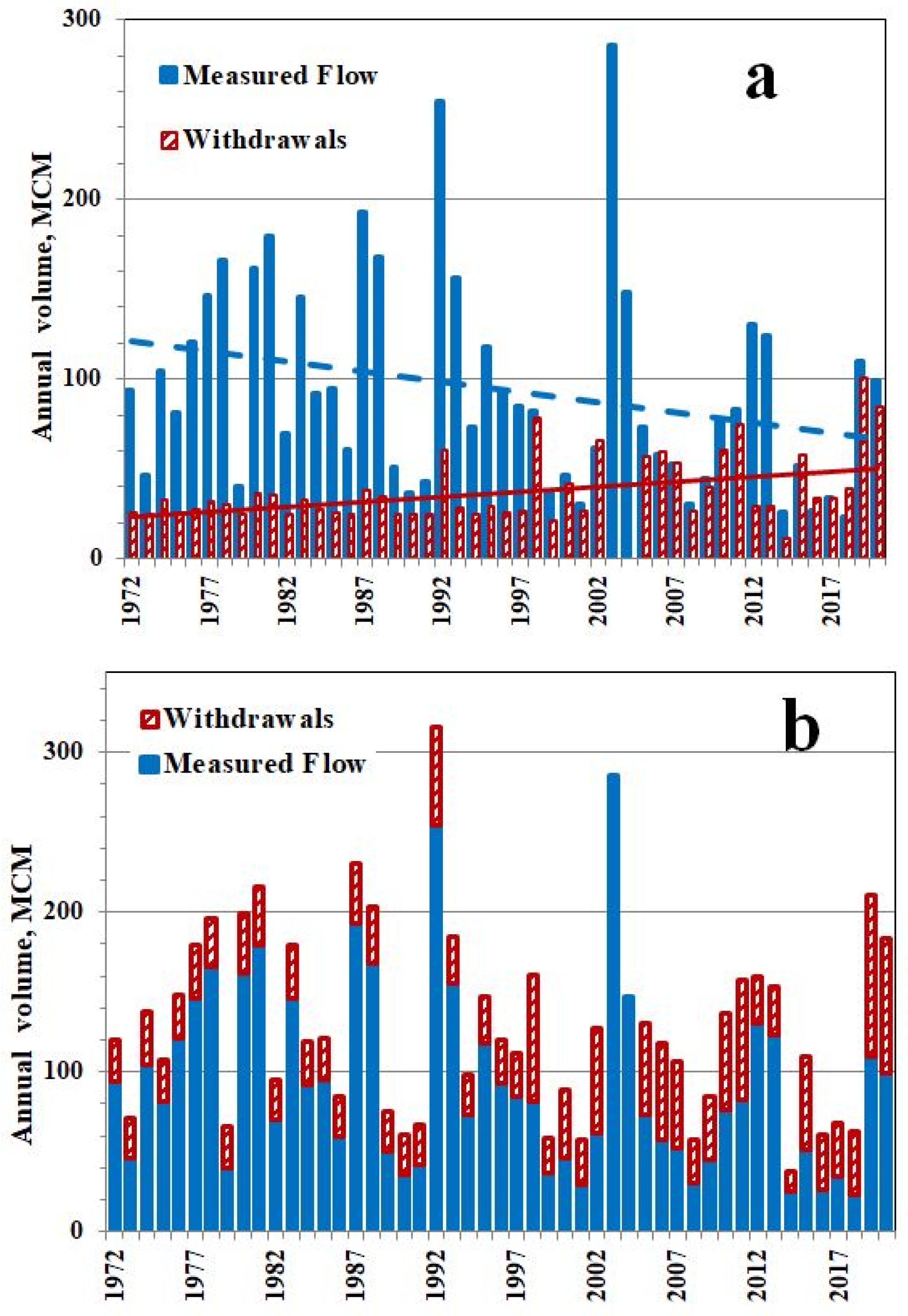
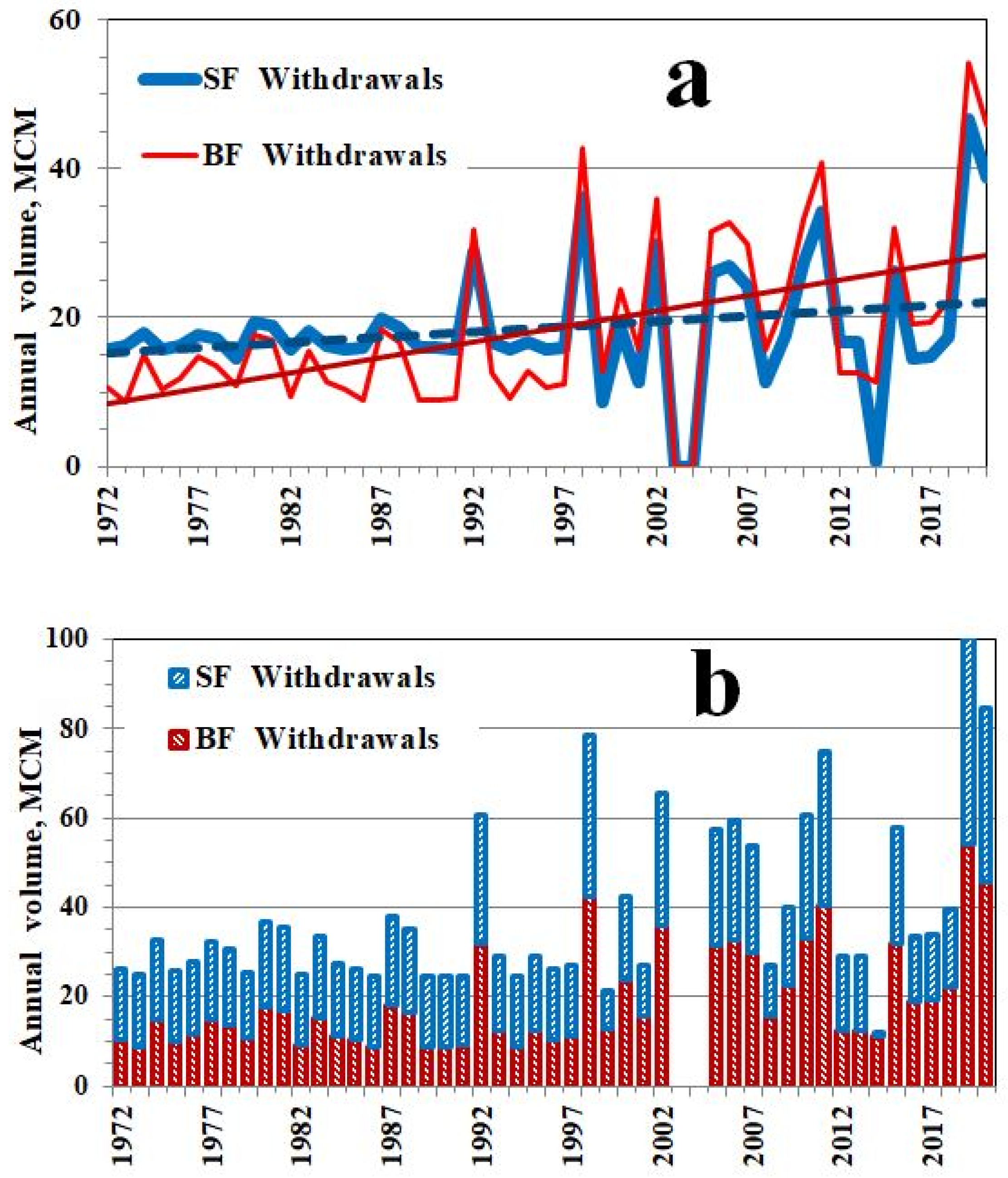
The FAO declared that it is practically impossible to determine the exact figure for groundwater abstraction in the Hasbani Basin [8]. By [26], the rough estimate (11 MCM/y) of the Hasbani water used in Lebanon for local irrigation and drinking water includes about 4.4 MCM/y of groundwater abstracted from licensed and unlicensed wells. Unlike it, in the present paper the total withdrawals from the Hasbani River are estimated (by the AWW method) at 30 MCM/y (1972–1983) and 48 MCM/y (2008–2020) including respectively 13 MCM/y and 26 MCM/y as the base flow component (Table 2 and Table 6). The latter increase is undoubtedly caused by increased number of private (mainly unregistered) wells. By indirect indices (areas of irrigated land, population, and water consumption rates), the total (irrigation and domestic) water use in the Hasbani Basin (before 2011) is estimated as no less than 29 MCM/y (Section 5.3). This figure supports value of 34 MCM/y which in the present study is the calculated water withdrawals for 1972–2010.

It should be noted that water withdrawals estimated in this study are of the same order as Lebanon’s share of Jordan River water use (of 35 MCM/y) under the Johnston Plan Allocation. The Johnston Plan (referring only to surface flow) was proposed to the riparian countries in 1955 but was never ratified. Nevertheless, it became a benchmark for water management and negotiations in the Jordan River basin [1,65,68].

Substantial issues for further consideration are: (i) What water withdrawals means? (ii) how efficiently the abstracted water is used? and (iii) which part of the water use has been accounted for in published estimates (as stated above, incomplete, rough and etc.,)? The answer to the first question is discussed in the next section. Regarding the second question, a large share of water in the distribution systems is lost through leakages (partly recharging the local aquifer). FAO reported 35–50% seepage from the public water supply networks in Lebanon [8]. One would not expect a better situation in the private sector. The answer to the third question remains uncertain.

6.2. Flow Trend Attribution: What Are Water Withdrawals?

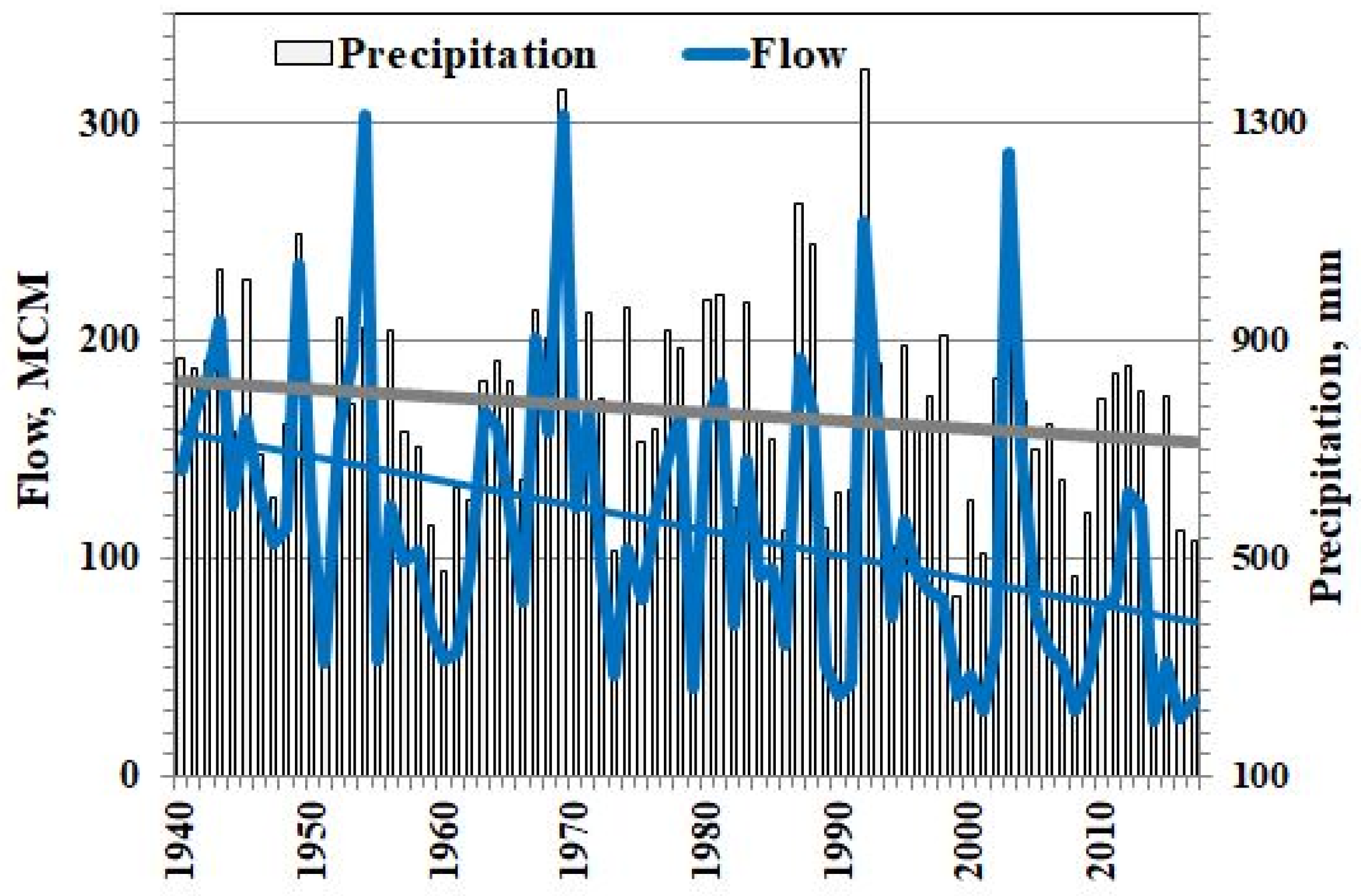
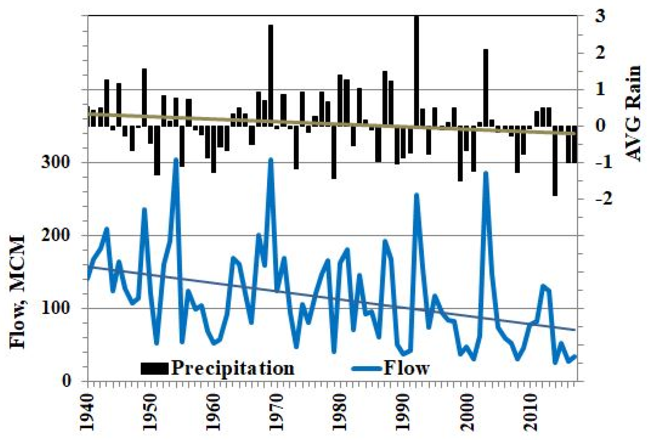
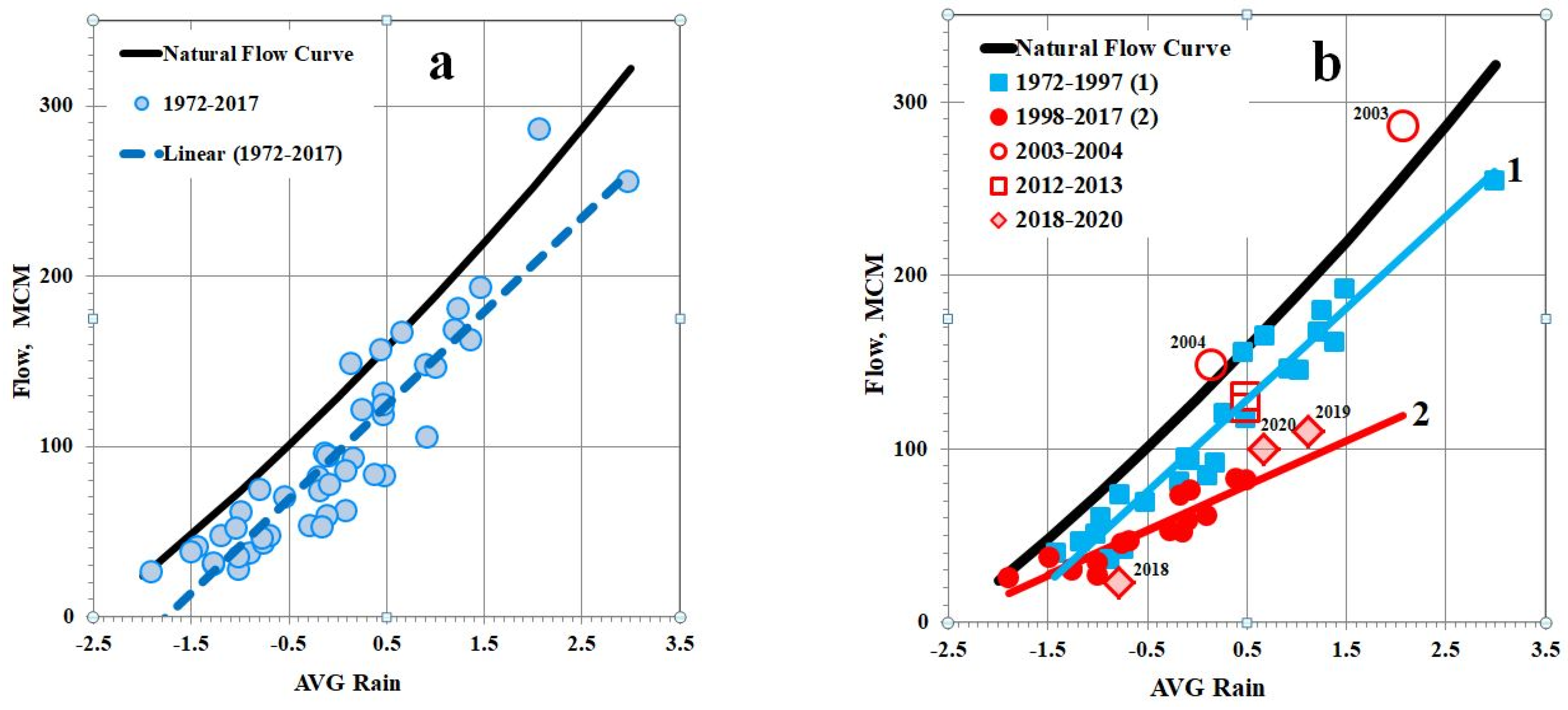
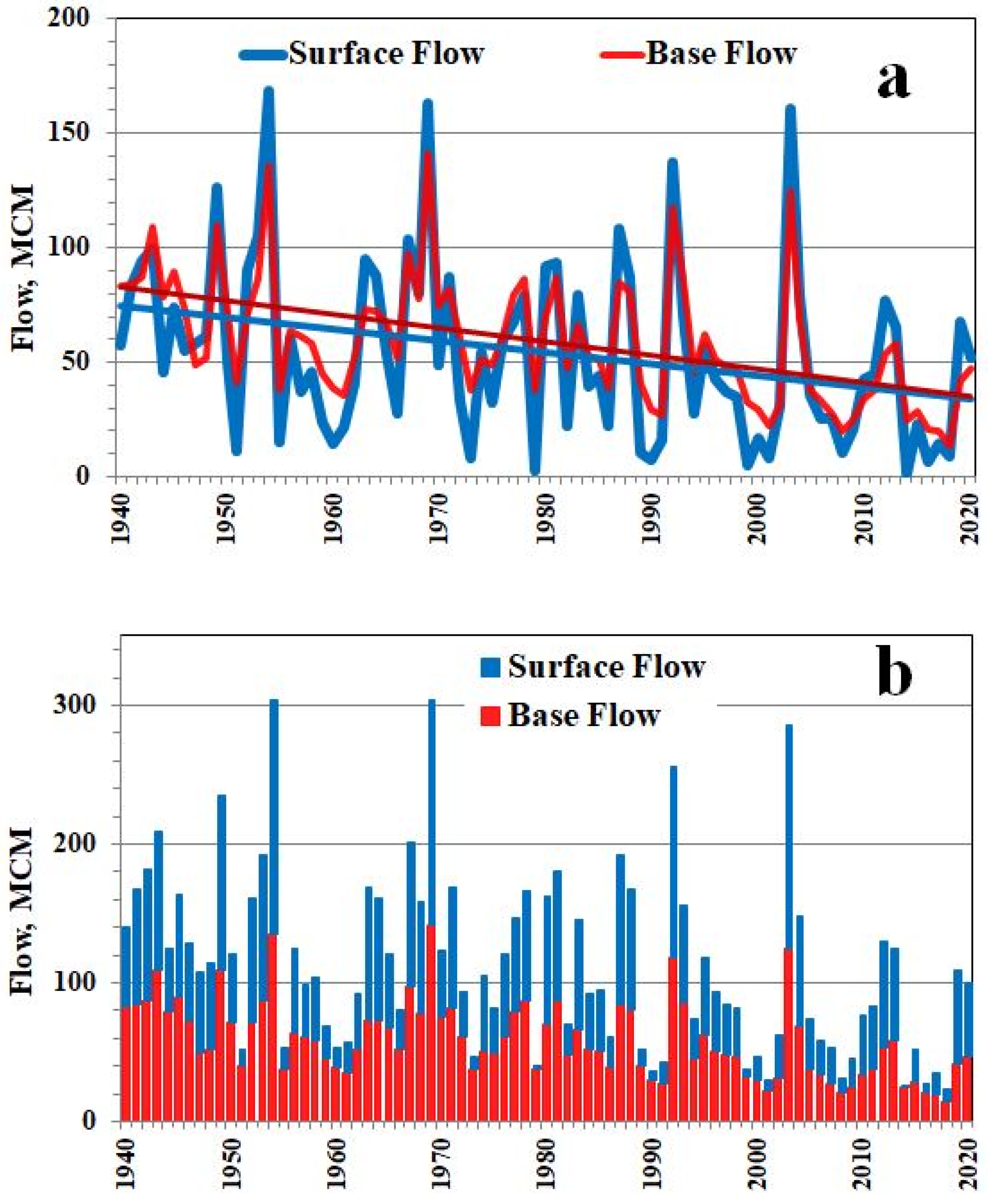
In the present study, the statistically significant decreasing trend in precipitation and flow of the Hasbani River, as well as the relationship between them is detected and confirmed. This means that a decrease in precipitation (climate signal) can be considered as an obvious driving force behind a decrease in flow. But this driver is not the only one, as the drop in flow exceeds the decreasing trend in precipitation.

Further analysis revealed the dynamic nature of the PF relationship, which indicated a consistent flow decline in subsequent sub-periods when with the same precipitation in the basin, less and less runoff was measured at the downstream station. Most likely, this effect is associated with some water withdrawals primarily caused by human activities in the basin (development of irrigation, economic needs, etc.,). However the influence of other factors is not excluded. So far, we used the term “withdrawals” without detailed interpretation, assuming (by the AWW method definition) that withdrawals are the total amount of water removed from the river (or did not reach it) and not included in the measured flow. Estimates of indirect indices (irrigated land area, population, and water consumption rates) confirmed that water use is a significant driving force behind a decrease in the Hasbani flow and almost completely explains the amount of water withdrawals. Attributing flow changes to other specific drivers (apart from decrease in precipitation and developing water use) is discussed further in this section.

First of all, this refers to the global air warming hypothesis, according to which increase in air temperature leads to increase in evapotranspiration and decrease in flow. For the Jordan River headwaters, potential evapotranspiration (PET) was estimated from daily minimum and maximum temperature data in the Har Qnaan weather station along with extraterrestrial solar radiation [19,69]. While rising temperature in the basin is statistically significant and the calculated annual PET increases from 1130 mm in 1984–1988 to 1160 mm in the 2007–2016 period, this change (about 2.6%) is too small to explain meaningfully the observed streamflow decreases. This is confirmed by the following simplified calculation. If the change in PET (2.6%) is roughly (as an upper and unrealistically high limit) attributed to the actual annual evapotranspiration (ET) in the Hasbani Basin (from 226 mm [16] to 238 mm [70]), then the increase in ET is estimated as less than 5–6 mm (or 3–4 MCM) for 1984–2016 period. This means that global air warming can be considered as only a secondary driver for reducing the Hasbani flow (in compare with Figure 2 and Table 2).

In the present study, the latter conclusion is confirmed by assessing the possible impact of the global air warming on the Hasbani surface flow decrease. This effect can be estimated as not higher than 1 MCM during 1972–2007, assuming that it only caused a slight increase in surface flow withdrawals during this period (Table 6).

Further, the influence of previous dry years on the Hasbani flow decrease was considered as a possible driver. Such effect of “hydrological memory” (or “drought hypothesis”) was found for incoming water to the Lake Kinneret [10,71] and for the Dan spring flow [9,16] (in consideration of one previous year and three previous years, respectively). In the present case, such effect could be real due to the facts that more than half of the Hasbani basin area is represented by karst exposures and the river is fed mainly by springs. The impact of the previous dry year on flow and water withdrawals in the current year was analyzed within the AWW method. As a result, a slight tendency was revealed, which turned out to be statistically insignificant against the influence of water use.

Summing up the above discussion, the following can be argued:

-

Decrease in precipitation (climate signal) and human activities in the basin (anthropogenic factor) are the main driving forces behind a decrease in the Hasbani flow.

-

Global air warming can be considered only as a secondary driver for reducing the Hasbani flow.

-

Water withdrawals from the Hasbani River estimated by the AWW method are generally results of the human water use with a negligible contribution due to global air warming.

Thus, the estimates of water withdrawals and water use are quite comparable. Moreover, it is quite possible to assume that for water resources management or for assessing the water balance in a transboundary basin, it can be more important to assess exactly withdrawals (as a water deficit) than the water consumption.

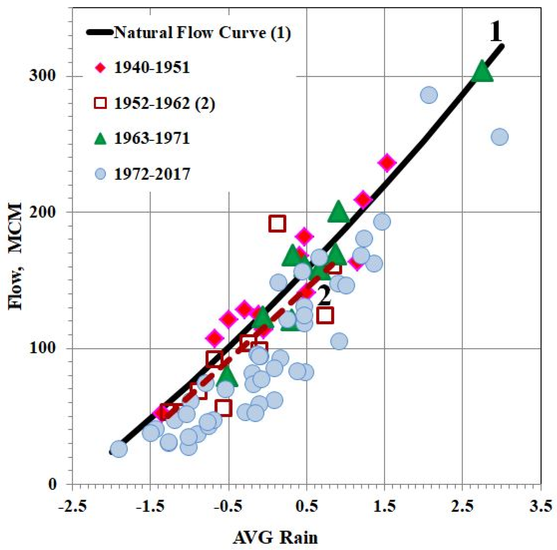
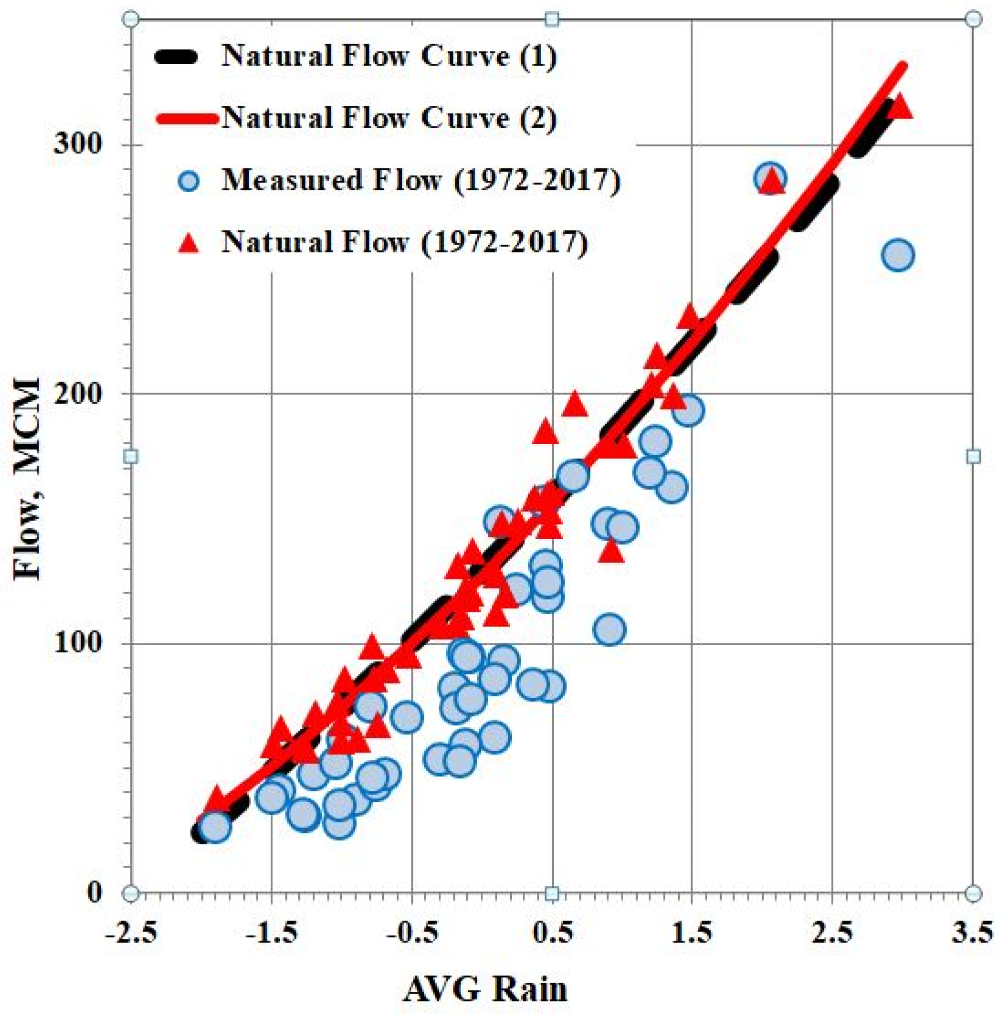
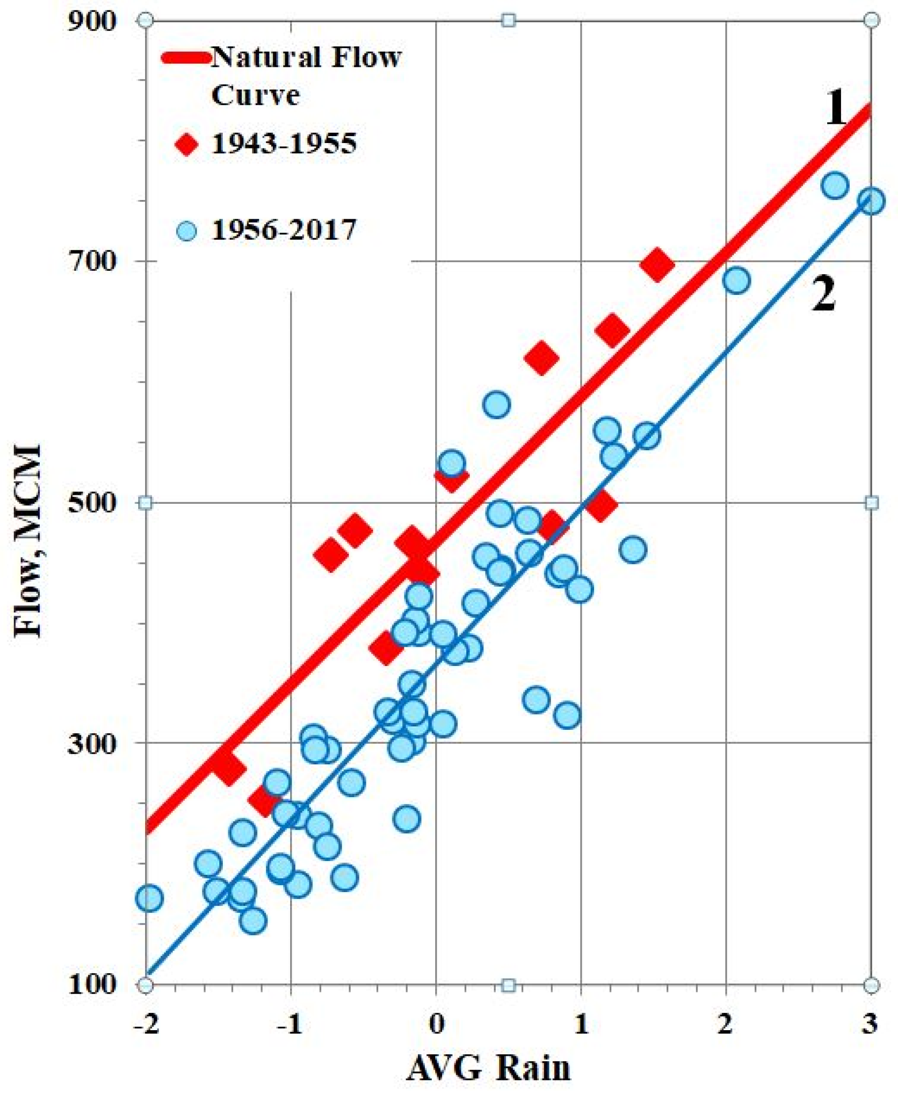
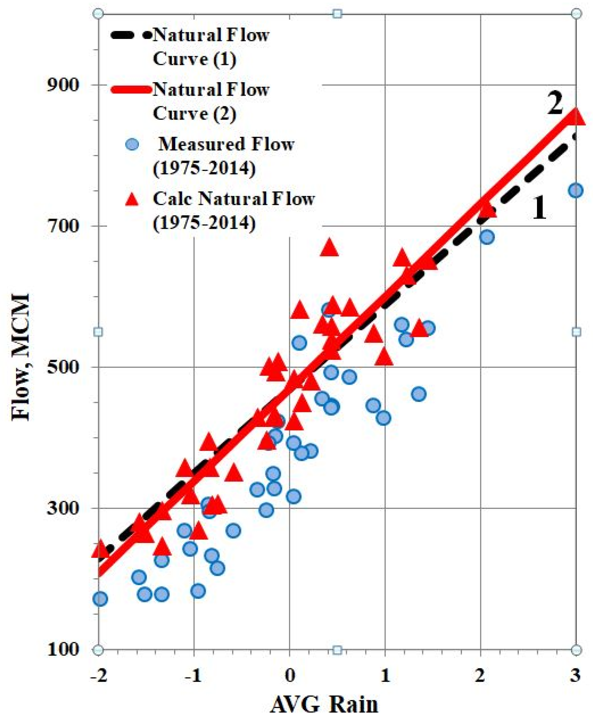
It is important to reiterate that the AWW method enables to differentiate between climatic and anthropogenic impacts on the river flow decrease. This follows from the definition of the AWW method, since the dynamics of the precipitation–flow relationship is analyzed, and not only the trend to a decrease in the flow. Therefore the present study enabled to estimate the relative contribution of two main drivers to the observed decrease of flow. As it was confirmed, a decrease in precipitation is an obvious driving force behind a decrease in the Hasbani flow. Correlation coefficient (R) between precipitation and measured flow (1972–2020) is 0.918, i.e., this driver describes 84% of variance (or dispersion, D) of flow. For natural flow (sum of measured flow and calculated withdrawals) these values are estimated as R = 0.974 and D = 95%, i.e., 11% more taking into consideration the water withdrawals as a balance component of flow.

On the other hand, regarding results of trend analysis, the statistically significant decrease in precipitation and flow of the Hasbani River (1972–2020) was detected as following: for precipitation–15%; for measured flow–45%; and for natural flow (sum of measured flow and calculated withdrawals–19%. As can be seen, in the absence of water withdrawals, the drop in natural flow would be slowed by 26% compared to the trend in measured flow and would approach the trend in precipitation. The latter (i) provides evidence that in this case water use is a more responsible driver in reducing flow than precipitation, and (ii) serves (together with Figure 7) as verification of the AWW method applied to the Hasbani River.

7. Conclusions and Recommendations

In the present study, the AWW method was proposed as a nonstandard solution to the problem of assessing water withdrawals in the scarce-data transboundary basin. The method operates with the open-source available data on precipitation and river flow and thereby overcomes the usual restriction due to lack of data on shared water use in the Middle East. Analysis of dynamic precipitation-flow relationships enabled to separate the effect of water withdrawals from the total decline of river flow under the decreasing precipitation.

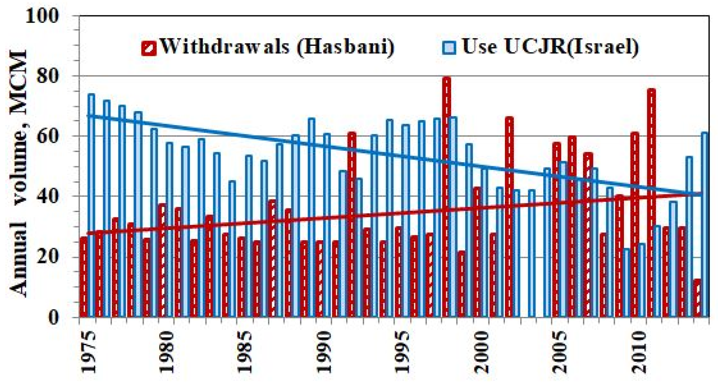
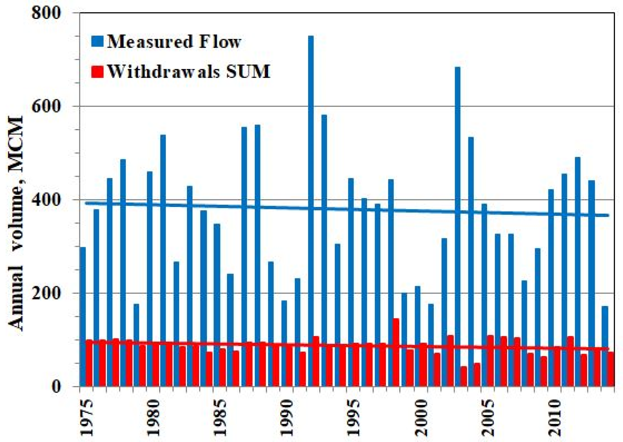
According to the published sources, the present study is the first which provided the complete and rather detailed estimates of water withdrawals from total, surface, and groundwater flow of the Hasbani River in Lebanon (1972–2020). The obtained estimates were confirmed by indirect indices such as area of the irrigated agricultural land and population in the Hasbani Basin. The strong argument in support of the results was validation of the AWW method based on the independent data on water use in the Israeli part of Upper Catchments of the Jordan River (1975–2014, Israel Water Authority).

Careful study revealed and confirmed that (i) decrease in precipitation (climate signal) and developed human activities in the basin (anthropogenic factor) are the main driving forces behind a decrease in the Hasbani flow, and (ii) water withdrawals estimated by the AWW method are generally the results of water use with a negligible contribution of increase in evapotranspiration due to global air warming.

The results of the study are useful for water balance estimations, as well as for management of water resources in the Jordan River headwaters basin and in the entire Lake Kinneret Basin.

The current research should not be regarded only as a regional study but it offers a general approach to solving similar problems. The AWW method can be applied to other transboundary basins under conditions of uncertain (or limited) data on water use, but subject both to the available precipitation and flow data and to confirmation of main hypotheses formulated in Section 3.2.

The AWW method enables historical and real-time monitoring of water withdrawals in any riparian state and in the entire transboundary basin. Undoubtedly, reliable data on water demand and water use should be the necessary basis for settlement of problematic transboundary water relations, especially within the current critical situation in the Middle East due to expanding geopolitical, socio-economic, and humanitarian problems.

In order to maintain the transparency and reproducibility of the research, “Supplementary File.xlsx” is available online at www.mdpi.com/xxx/s1.

References

1. UN-ESCWA (United Nations Economic and Social Commission for Western Asia); BGR (Bundesanstalt für Geowissenschaften und Rohstoffe). Jordan River Basin. In Inventory of Shared Water Resources in Western Asia; United Nations Economic and Social Commission for Western Asia: Beirut, Lebanon, 2013; Chapter 6. [Google Scholar]
2. Hussein, H.; Grandi, M. Dynamic political contexts and power asymmetries: The cases of the Blue Nile and the Yarmouk Rivers. Int. Environ Agreem. 2017, 17, 795. [Google Scholar] [CrossRef] [Green Version]
3. Suleiman, R. The Historical Evolution of the Water Resources Development in the Jordan River Basin in Jordan; MREA–IWMI Working Paper; French Regional Mission for Water and Agriculture: Amman, Jordan, 2004. [Google Scholar]
4. Aggestam, K. Desecuritisation of water and the technocratic turn in peacebuilding. Int. Environ. Agreem. Politics Law Econ. 2015, 15, 327–340. [Google Scholar] [CrossRef]
5. Avni, N.; Fishbain, B.; Shamir, U. Water consumption patterns as a basis for water demand modeling. Water Resour. Res. 2015, 51, 8165–8181. [Google Scholar] [CrossRef] [Green Version]
6. Weinthal, E.; Zawahri, N.; Sowers, J. Securitizing water, climate, and migration in Israel, Jordan, and Syria. Int. Environ. Agreem. Politics Law Econ. 2015, 15, 293–307. [Google Scholar] [CrossRef]
7. Wine, M.L. Under non-stationarity securitization contributes to uncertainty and tragedy of the commons. J. Hydrol. 2019, 568, 716–721. [Google Scholar] [CrossRef]
8. FAO (Food and Agriculture Organization of the United Nations). Irrigation in the Middle East Region in Figures: AQUASTAT Survey—2008; FAO Water Reports; Food and Agriculture Organization of the United Nations: Rome, Italy, 2009; p. 34. [Google Scholar]
9. Givati, A.; Rosenfeld, D. Possible impacts of anthropogenic aerosols on water resources of the Jordan River and the Sea of Galilee. Water Resour. Res. 2007, 43, W10419. [Google Scholar] [CrossRef]
10. Rimmer, A.; Givati, A.; Samuel, R.; Alpert, P. Using ensemble of climate models to evaluate future water and solutes budgets in Lake Kinneret, Israel. J. Hydrol. 2011, 410, 248–259. [Google Scholar] [CrossRef]
11. Givati, A.; Rosenfeld, D.; Lynn, B.; Lui, Y.; Rimmer, A. Using the high resolution WRF model for calculating stream flow in the Jordan River. J. Appl. Meteorol. Climatol. 2012, 51, 285–298. [Google Scholar] [CrossRef]
12. Shaban, A. Indicators and aspects of hydrological drought in Lebanon. Water Resour. Manag. 2009, 23, 1875–1891. [Google Scholar] [CrossRef]
13. Markel, D.; Shamir, U.; Green, P. Operational management of Lake Kinneret and its watershed. In Lake Kinneret: Ecology and Management; Zohary, T., Sukenik, A., Berman, T., Nishri, A., Eds.; Springer: Dordrecht, The Netherlands, 2014; pp. 541–560. [Google Scholar]
14. Halfon, N.; Levin, Z.; Alpert, P. Temporal rainfall fluctuations in Israel and their possible link to urban and air pollution effects. Environ. Res. Lett. 2009, 4. [Google Scholar] [CrossRef]
15. Shohami, D.; Dayan, U.; Morin, E. Warming and drying of the eastern Mediterranean: Additional evidence from trend analysis. J. Geophys. Res. 2011, 116, D22101. [Google Scholar] [CrossRef]
16. Rimmer, A.; Salingar, Y. Modelling precipitation-streamflow processes in karst basin: The case of the Jordan River sources, Israel. J. Hydrol. 2006, 331, 524–542. [Google Scholar] [CrossRef]
17. Rimmer, A.; Givati, A. Hydrology. In Lake Kinneret—Ecology and Management; Aquatic Ecology Series; Zohary, T., Sukenik, A., Berman, T., Nishri, A., Eds.; Springer: Cham, Switzerland, 2014; Chapter 7; p. 6. [Google Scholar] [CrossRef]
18. Sade, R.; Rimmer, A.; Samuels, R.; Salingar, Y.; Denisyuk, M.; Alpert, P. Water Management in a Complex Hydrological Basin—Application of Water Evaluation and Planning Tool (WEAP) to the Lake Kinneret Watershed, Israel. In Integrated Water Resources Management: Concept, Research and Implementation; Borchardt, D., Bogardi, J.J., Ibisch, R.B., Eds.; Springer: Cham, Switzerland, 2016; Chapter 2. [Google Scholar] [CrossRef]
19. Wine, M.L.; Rimmer, A.; Laronne, J.B. Agriculture, diversions, and drought shrinking Galilee Sea. Sci. Total Environ. 2019, 651, 70–83. [Google Scholar] [CrossRef] [PubMed]
20. Shentsis, I.; Inbar, N.; Rosenthal, E.; Magri, F. Assessing water consumption and aquifer discharge through springs based on the joint use of rain and flow data in the Yarmouk River Basin. Environ. Earth Sci. 2019, 78, 1–10. [Google Scholar] [CrossRef]
21. Kenny, J.F.; Barber, N.L.; Hutson, S.S.; Linsey, K.S.; Lovelace, J.K.; Maupin, M.A. Estimated Use of Water in the United States in 2005; Circular 1344; U.S. Geological Survey: Reston, VA, USA, 2009; p. 52.
22. Haie, N. Transparent Water Management Theory: Sefficiency in Sequity; Springer: Singapore, 2020; p. 134. [Google Scholar] [CrossRef]
23. Gilad, D.; Schwartz, S. Hydrogeology of the Jordan Sources Aquifers; Israel Hydrological Service Report Hydro/5/78; Hydrological Service: Jerusalem, Israel, 1978; pp. 1–58. (In Hebrew) [Google Scholar]
24. Simpson, B.; Carmi, I. The hydrology of the Jordan tributaries (Israel): Hydrographic and isotopic investigation. J. Hydrol. 1983, 62, 225–242. [Google Scholar] [CrossRef]
25. Comair, G.F. A new Approach for Water Planning, Management and Conflict Resolutions in Lebanese Transboundary Basins: Hydrologic Modeling for Climate Variation and Water Policy Development. Ph.D. Thesis, University of Texas, Austin, TX, USA, 2013. [Google Scholar]
26. Zeitoun, M.; Eid-Sabbagh, K.; Dajani, M.; Talhami, M. Hydro-Political Baseline of the Upper Jordan River; Association of the Friends of Ibrahim Abd el Al (AFIAL): Beirut, Lebanon, 2012. [Google Scholar]
27. Baroud, Z.; El-Alayli, G.; Abdallah, C.; Zeitoun, M. Legal Analysis of Transboundary Waters in the Upper Jordan River Basin; AFIAL: Beirut, Lebanon, 2014. [Google Scholar] [CrossRef]
28. Mason, M.; Khawlie, M. Fluid sovereignty: State-nature relations in the Hasbani Basin, southern Lebanon. Ann. Am. Assoc. Geogr. 2016, 106, 1344–1359. [Google Scholar] [CrossRef] [Green Version]
29. Merz, B.; Vorogushyn, S.; Uhlemann, S.; Delgado, J.; Hundecha, Y. HESS opinions “More efforts and scientific rigour are needed to attribute trends in flood time series”. Hydrol. Earth Syst. Sci. 2012, 16, 1379–1387. [Google Scholar] [CrossRef] [Green Version]
30. Kirkwood, B.R.; Sterne, J. Essential Medical Statistics, 2nd ed.; Blackwell Science: Oxford, UK, 2003; p. 288. [Google Scholar]
31. Dodge, Y. The Oxford Dictionary of Statistical Terms; Oxford University Press: New York, NY, USA, 2003; p. 512. ISBN 0-19-920613-9. [Google Scholar]
32. Johnson, R.; Wichern, W. Applied Multivariate Statistical Analysis, 6th ed.; Pearson/Prentice Hall International: Hoboken, NJ, USA, 2007; p. 773. ISBN 0-13-187715-1. [Google Scholar]
33. Shentsis, I.; Inbar, N.; Magri, F.; Rosenthal, E. Numerical representation of rainfall field in basins of the Upper Jordan River and of the Yarmouk River. Environ. Earth Sci. 2018, 77, 1–17. [Google Scholar] [CrossRef]
34. Ministry of Agriculture, Water Commission. Hydrological Year-Book of Israel—Summary of records prior to October 1967; Ministry of Agriculture, Water Commission, Hydrological Service: Jerusalem, Israel, 1971.
35. Water Authority, Hydrological Service. Hydrological Year-Book of Israel; Water Authority, Hydrological Service: Jerusalem, Israel, 1963–2018; ISSN 0073-4217. [Google Scholar]
36. Sapir, G.; Sagi, O. Estimating the Quantities of Water Which Do Not Reach the Lake Kinneret due to Human Use in the Watershed; Final Report 2014; by Funding support from Israel Water Authority; DHV MED Ltd.: Jerusalem, Israel, 2014. (In Hebrew) [Google Scholar]
37. Ministry of Energy and Water in Lebanon (MEW). Country Consultation with the Republic of Lebanon. In Country Consultations for the Inventory of Shared Water Resources in Western Asia; Ministry of Energy and Water in Lebanon: Beirut, Lebanon, 2012. [Google Scholar]
38. Ministry of Agriculture in Lebanon; Food and Agriculture Organization of the United Nations (FAO). Atlas Agricole du Liban—Projet D’assistance au Recensement Agricole; Food and Agriculture Organization of the United Nations: Rome, Italy, 2005.
39. Merheb, M. Watershed Management of the Hazbani-Wazani. Master’s Thesis, Université Libanaise, Beirut, Lebanon, 2010. [Google Scholar]
40. Ministry of Environment (MOE). Lebanon State of the Environment: National Standards for Environmental Quality; SPASI Project, Funded by EU; Ministry of Environment: Beirut, Lebanon, 2001.
41. World Bank. Republic of Lebanon—Water Sector: Public Expenditure Review. Washington. 2010. Available online: http://documents.worldbank.org/curated/en/965931468265767738 (accessed on 1 May 2018).
42. Government of Lebanon (GOL). Service Area of Hasbani Watercourse; Position Report 09, October 2002; Government of Lebanon: Beirut, Lebanon, 2002.
43. MoSA; UNDP. Development of Mapping of Living in Lebanon 1995–2004: A Comparison with the Results of “Mapping of Living Conditions in Lebanon, 1998”, a part of the “Capacity Building for Poverty Reduction” joint project between Ministry of Social Affairs and United Nations Development Programme; UNDP: Beirut, Lebanon, 2007. [Google Scholar]
44. MEDA. Plan de Development Pour le Basin Versant du Hasbani Wazzani: Rapport de Synthese de la Phase 2. Investment Planning Programme (IPP) No. Meda LBN 4100/1B/96/111. Beirut, European Union—Meda, with Partex-Thales-Sema Consortium. 2003. Available online: http://www.agriculture.gov.lb/ATLAS_%20AGRICOLE/atlas.html (accessed on 1 May 2018).
45. CAS (Central Administration of Statistics). Census of Buildings Dwellings and Establishments (CBDE). Lebanon; 2004. Available online: http://www.cas.gov.lb/index.php?option=com_content&view=article&id=54&Itemid=37 (accessed on 1 May 2018).
46. Eldawy, D. A Fragile Situation: Will the Syrian Refugee Swell Push Lebanon over the Edge? Migration Policy Institute (MPI). 21 February 2019. Available online: https://www.migrationpolicy.org/article/syrian-refugee-swell-push-lebanon-over-edge (accessed on 10 July 2020).
47. Farajalla, N. Impact of Syrian refugees on Lebanon’s water resources. In Water, Migration and How They are Interlinked; Working paper 27; Jägerskog, A., Swain, A., Eds.; SIWI: Stockholm, Sweden, 2016. [Google Scholar]
48. Nathan, R.J.; McMahon, T.A. Evaluation of automated techniques for base flow and recession analyses. Water Resour. Res. 1990, 26, 1465–1473. [Google Scholar] [CrossRef]
49. Chapman, T. A comparison of algorithms for stream flow recession and base flow separation. Hydrol. Process 1999, 13, 701–714. [Google Scholar] [CrossRef]
50. Mugo, J.M.; Sharma, T.C. Application of a conceptual method for separating runoff components in daily hydrographs in Kimakia Forest Catchments, Kenya. Hydrol. Process. 1999, 13, 2931–2939. [Google Scholar] [CrossRef]
51. Tan, S.B.K.; Lo, E.Y.; Shuy, E.B.; Chua, L.H.C.; Lim, W.H. Generation of total runoff hydrographs using a method derived from a digital filter algorithm. J. Hydrol. Eng. 2009, 14, 101–106. [Google Scholar] [CrossRef]
52. Ladson, A.R.; Brown, R.; Neal, B.; Nathan, R. A standard approach to base flow separation using the Lyne and Hollick filter. Aust. J. Water Resour. 2013, 17, 25–34. [Google Scholar] [CrossRef]
53. Smakhtin, V.U. Estimating continuous monthly baseflow time series and their possible applications in the context of the ecological reserve. Water SA 2001, 27, 213–217. [Google Scholar] [CrossRef] [Green Version]
54. Eckhardt, K. How to construct recursive digital filters for baseflow separation. Hydrol. Process. 2005, 19, 507–515. [Google Scholar] [CrossRef]
55. Wahl, K.L.; Wahl, T.L. Determining the Flow of Comal Springs at New Braunfels, Texas; U.S. Geological Survey: Reston, VA, USA; United States Bureau of Reclamation: Lakewood, CO, USA, 1995; pp. 1–10.
56. Gustard, A.; Bullock, A.; Dixon, J.M. Low Flow Estimation in the United Kingdom; IH Report No.108; Institute of Hydrology: Wallingford, UK, 1992; p. 88.
57. Lott, D.A.; Stewart, M.T. Base flow separation: A comparison of analytical and mass balance methods. J. Hydrol. 2016, 535, 525–533. [Google Scholar] [CrossRef]
58. Chapman, T.G. Comment on ‘Evaluation of automated techniques for base flow and recession analysis’ by R.J. Nathan and T.A. McMahon. Water Resour. Res. 1991, 27, 1783–1784. [Google Scholar] [CrossRef]
59. Furey, P.R.; Gupta, V.K. A physically based filter for separating base flow from streamflow time series. Water Resour. Res. 2001, 37, 2709–2722. [Google Scholar] [CrossRef] [Green Version]
60. Blume, T.; Zehe, E.; Bronstert, A. Rainfall—Runoff response, event-based runoff coefficients and hydrograph separation. Hydrol. Sci. J. 2007, 52, 843–862. [Google Scholar] [CrossRef]
61. Rice, K.C.; Hornberger, G.M. Comparison of hydrochemical tracers to estimate source contributions to peak flow in a small, forested, headwater catchment. Water Res. 1998, 34, 1755–1766. [Google Scholar] [CrossRef]
62. Hoeg, S.; Uhlenbrook, S.; Leibundgut, C. Hydrograph separation in a mountainous catchment—Combining hydrochemical and isotopic tracers. Hydrol. Processes 2000, 14, 1199–1216. [Google Scholar] [CrossRef]
63. Ladouche, B.; Probst, A.; Viville, D.; Idir, S.; Baque, D.; Loubet, M.; Probst, J.L.; Bariac, T. Hydrograph separation using isotopic, chemical and hydrological approaches (Strengbach catchment, France). J. Hydrol. 2001, 242, 255–274. [Google Scholar] [CrossRef]
64. Arnold, J.G.; Allen, P.M.; Muttiah, R.; Bernhardt, G. Automated base flow separation and recession analysis techniques. Ground Water 1995, 33, 1010–1018. [Google Scholar] [CrossRef]
65. Phillips, D.J.H.; Attili, S.; McCaffrey, S.; Murray, J.S. The Jordan River Basin: 1. Clarifications of the Allocations in the Johnston Plan. Water Int. 2007, 32, 16–38. [Google Scholar] [CrossRef]
66. Weinberger, G.; Givati, A.; Livshitz, Y.; Zilberbrand, M.; Tal, A.; Weiss, M.; Zurieli, A. The Natural Water Resources between the Mediterranean Sea and the Jordan River; Hydro Report 11/1; Israeli Hydrological Service: Jerusalem, Israel, 2012; ISSN 0334-3367.
67. Eid-Sabbagh, K.P. A Political Economy of Water in Lebanon: Water Resource Management, Infrastructure Production, and the International Development Complex. Ph.D. Thesis, University of London, London, UK, 2015. [Google Scholar]
68. Rosenthal, E.; Sabel, R. Water and Diplomacy in the Jordan River Basin. Israel. J. Foreign Aff. 2009, 3, 95–115. [Google Scholar]
69. Hargreaves, G.H.; Samani, Z.A. Reference crop evapotranspiration from temperature. Appl. Eng. Agric. 1985, 1, 96–99. [Google Scholar] [CrossRef]
70. Comair, G.F.; McKinney, D.C.; Siegel, D. Hydrology of the Jordan river basin: Watershed delineation, precipitation and evapotranspiration. Water Resour. Manag. 2012, 26, 4281–4293. [Google Scholar] [CrossRef]
71. Shentsis, I.; Ben-Zvi, A. Within–season updating of seasonal forecast of Lake Kinneret inflow. J. Hydrol. Eng. ASCE 1999, 4, 381–385. [Google Scholar] [CrossRef]
72. Yager, R.M.; Maurer, D.K.; Mayers, C.J. Assessing Potential Effects of Changes in Water Use with a Numerical Groundwater-Flow Model of Carson Valley, Douglas County, Nevada, and Alpine County, California; U.S. Geological Survey Scientific Investigations Report, 2012–5262; U.S. Geological Survey: Reston, VA, USA, 2012; p. 73.
73. Khan, H.F.; Yang, Y.C.E.; Ringler, C.; Wi, S.; Cheema, M.J.M.; Basharat, M. Guiding Groundwater Policy in the Indus Basin of Pakistan Using a Physically Based Groundwater Model. J. Water Resour. Plan. Manag. 2017, 143. [Google Scholar] [CrossRef]
74. Shih, D.S.; Chen, C.J.; Li, M.H.; Jang, C.S.; Chang, C.M.; Liao, Y.Y. Statistical and numerical assessments of groundwater resource subject to excessive pumping: Case study in Southwest Taiwan. Water 2019, 11, 360. [Google Scholar] [CrossRef] [Green Version]
75. Reeves, H.W.; Hamilton, D.A.; Seelbach, P.W.; Asher, A.J. Ground-Water-Withdrawal Component of the Michigan Water-Withdrawal Screening Tool; U.S. Geological Survey Scientific Investigations Report, 2009–5003; U.S. Geological Survey: Reston, VA, USA, 2009; p. 36.
76. Mann, H.B. Non-parametric tests against trend. Econometrica 1945, 13, 163–171. [Google Scholar] [CrossRef]
77. Kendall, M.G. Rank Correlation Methods, 4th ed.; Charles Griffin: London, UK, 1975. [Google Scholar]
78. Cohen, J.; Cohen, P.; West, S.G.; Aiken, L.S. Applied Multiple Regression/Correlation Analysis for the Behavioral Sciences, 3rd ed.; Lawrence Earlbaum Associates: Mahwah, NJ, USA, 2003. [Google Scholar]
Figure 1. General view of the study area (a) and watersheds in the Upper Jordan River Basin (b).
Water 13 01440 g001
Figure 2. Hasbani River flow at Mayan Barukh Station vs. precipitation gauged at Kfar Giladi Station with detected linear trends (1940–2017).
Water 13 01440 g002
Figure 3. Hasbani River flow at Mayan Barukh Station in comparison to precipitation (AVG Rain) with detected linear trends (1940-2017). Note: AVG Rain is the z-score standardized and averaged annual precipitation at Kfar Giladi and Golan Experimental stations.
Water 13 01440 g003
Figure 4. Natural Flow Curve for Hasbani (Snir) River as the precipitation–flow relationship for initial (unregulated) period (1940–1971 without 1952–1962). Points relating to sub-period 1952–1962 and the corresponding curve 2 are placed obviously lower due to hydrometrical problems. See note to Figure 3.
Water 13 01440 g004
Figure 5. Relationship between flow of the Hasbani River at Mayan Barukh Station and precipitation (1972–2017) in comparison with the Natural Flow Curve (a). The same graph but two sub-period curves are differentiated as 1 (1972–1997) and 2 (1998–2017 without 2003–2004 and 2012–2013). Years 2003–2004, 2012–2013 are indicated as nonstandard and 2018–2020 are independent data (b). See note to Figure 3.
Water 13 01440 g005
Figure 6. Estimated withdrawals in the Hasbani basin (Lebanon) vs. measured flow at Mayan Barukh Station (1972–2017) with detected trends (a). Natural flow of the Hasbani River as sum of measured flow and estimated water withdrawals (b).
Water 13 01440 g006
Figure 7. Verification of the AWW method (applied to the Hasbani River) by comparison between the different versions of the Natural Flow Curves which are based (1) on the measured unregulated flow (1940–1971) and (2) on the calculated Natural Flow (1972–2017) (as sum of measured flow and withdrawals).
Water 13 01440 g007
Figure 8. Upper Jordan River flow at Sede Nehemya Station vs. precipitation gauged at Kfar Giladi Station with detected linear trends (1943–2017).
Water 13 01440 g008
Figure 9. Estimated (by the AWW method) water withdrawals in the Hasbani Basin vs. water use in the UCJR basin (Israel) with detected linear trends (1975–2014).
Water 13 01440 g009
Figure 10. Entire water withdrawals (SUM) in the UCJR Basin vs. Upper Jordan flow measured at Sede Nehemya Station with detected linear trends (1975–2014).
Water 13 01440 g010
Figure 11. Relationship between flow of the Upper Jordan River measured at Sede Nehemya Station and precipitation (1943–2017). For the initial period (1943–1955) points and trend-line (1) of the corresponding PF relationship (Natural Flow Curve) are indicated by red color. For the rest period (1956–2017) points and trend-line (2) of the corresponding PF relationship are indicated by blue color.
Water 13 01440 g011
Figure 12. Relationship between flow of the Upper Jordan River at Sede Nehemya Station and precipitation (1975–2014) in comparison with different versions of the Natural Flow Curve. Every curve is a trend line of PF relationship based on the following flow data: (1)—measured flow in the earlier unregulated period (1943–1955), (2)—natural flow (1975–2014) calculated as sum of measured flow, withdrawals in Hasbani basin (Lebanon) and water use in UCJR (Israel).
Water 13 01440 g012
Figure 13. Examples of the flow separation for the Hasbani (Snir) River (1992–1997) by the one-parameter recursive digital filter (Equations (2) and (3)) at the monthly time-scale (in the present study) (a). Model HYMKE [16]: draft of separated hydrograph (b) and hydrographs (1992–2000) presented results of an application of the daily two-parameter recursive digital filter to the Hasbani (Snir) River (c).
Water 13 01440 g013
Figure 14. Separated surface and base flow of the Hasbani River with detected trends (1940–2020) (a). Measured flow of the Hasbani River as sum of surface and base flow for the same period (b).
Water 13 01440 g014
Figure 15. Relationship between surface flow of the Hasbani River at Mayan Barukh Station and precipitation (1972–2017) in comparison with Natural Flow Curve (1940–1971). Two sub-period curves are differentiated as 1 (1972–1997) and 2 (1998–2017 without 2003–2004 and 2012–2013). Years 2003-2004, 2012-2013 are indicated as nonstandard and 2018-2020 are independent data (a). The same graph for base flow (b). See note to Figure 3.
Water 13 01440 g015
Figure 16. Surface and base flow withdrawals with detected linear trends (1972–2020) (a). Total withdrawals from the Hasbani River as sum of both components (1972–2020) (b).
Water 13 01440 g016