
Optimal Allocation of Surface Water Resources at the Provincial Level in the Uzbekistan Region of the Amudarya River Basin

 ,
,  and
and
Abstract
:1. Introduction
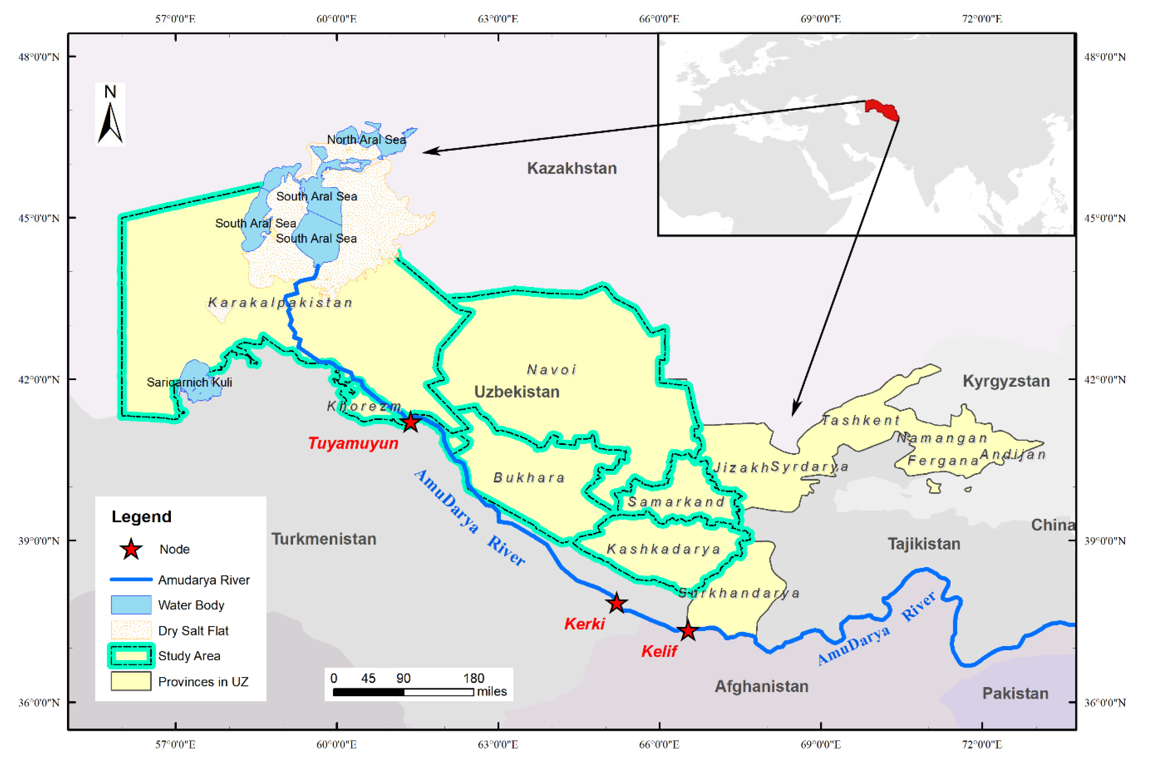
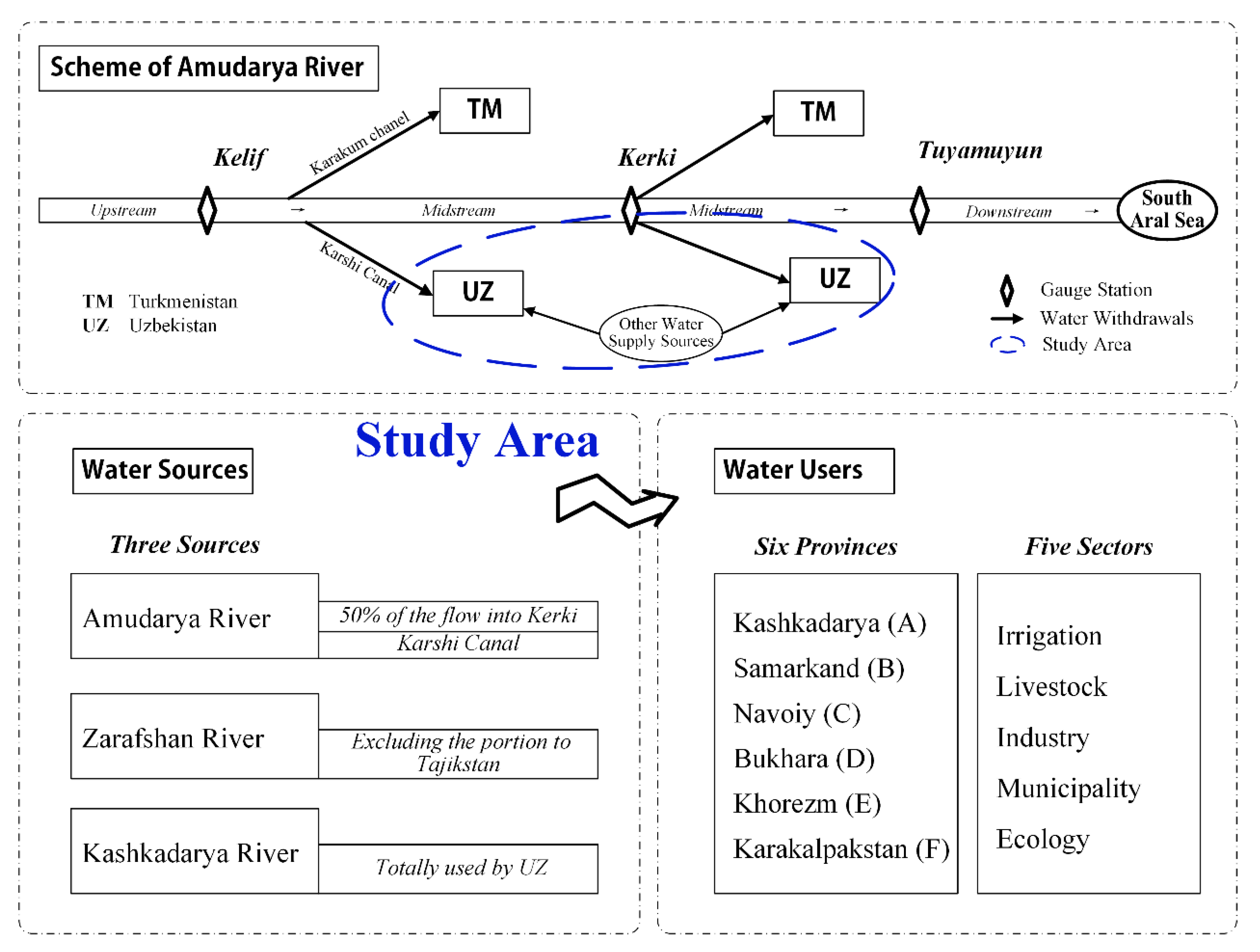
2. Study Area
3. Data and Methods
3.1. Data Collection
3.2. ITSP Method
- i = water user sector, i = 1,2,…,m, and m = 5 (irrigation; livestock; industry; municipality; ecology);
- j = province, j = 1,2,…,n, and n = 6 (Kashkadarya; Samarkand; Navoi; Bukhara; Khorezm; Karakalpakstan);
- k = the flow level available, k = 1,2,…,l, and l = 5 (high; high–medium; medium; medium–low; low);
- f = expected net system economic benefit over one year (thousand USD);
- Bij = the net benefit to user i in province j per unit of allocated water (USD/103 m3);
- Cij = the reduction of net benefit to user i in province j per unit of water not delivered (USD/103 m3);
- Wij = the fixed allocation target for water that is promised to user i in province j;
- Wijmax = the water demand for user i in provice j;
- pk = the probability of occurrence for different flow levels, and ;
- qk = the water availability under the flow level of k;
- Sijk = the amounts by which the water allocation targets (Wij) are not met when the flows are under the flow level of k.
4. Preparation of Input Data
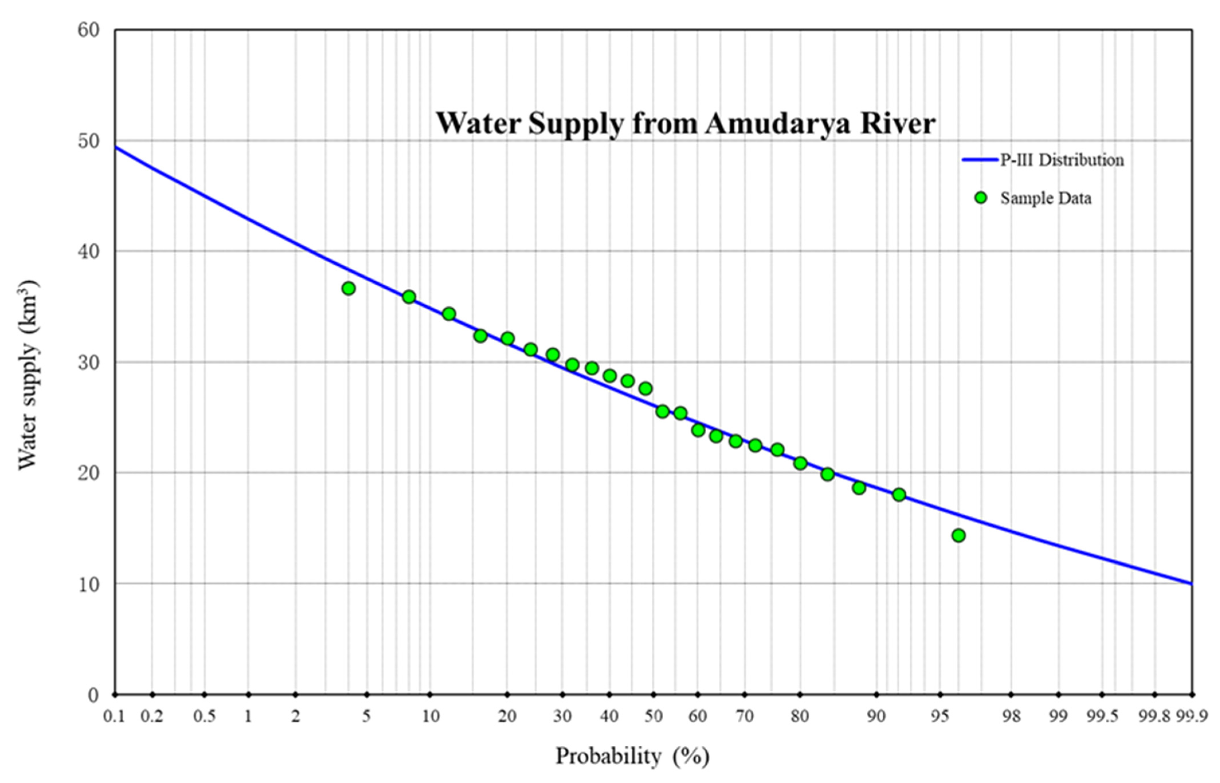
4.1. Water Supply and Water Demand
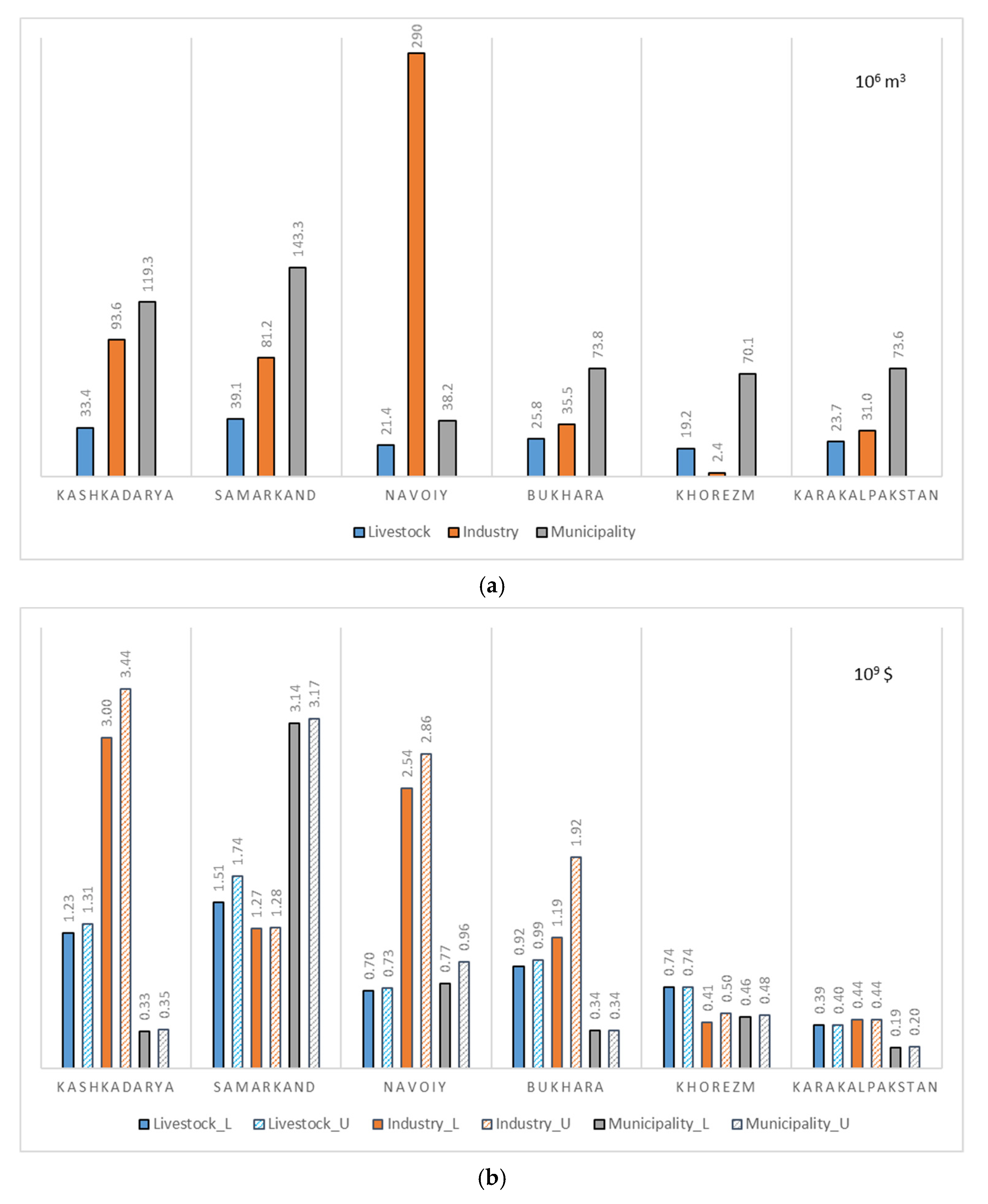
4.2. Coefficient of Economic Benefit and Economic Penalty
5. Results
5.1. Water Shortage by Supply–Demand Balance Analysis
5.2. Water Allocation Schemes under Maximization of Economic Benefits
5.3. Comparison with the Actual Water Allocation Schemes
6. Discussion
6.1. Optimized Water Distribution among Sectors
6.2. Optimized Water Distribution among Provinces
6.3. Optimized Water Allocation for Ecology
7. Conclusions
Author Contributions
Funding
Institutional Review Board Statement
Informed Consent Statement
Data Availability Statement
Conflicts of Interest
References
- Porkka, M.; Kummu, M.; Siebert, S.; Flörke, M. The Role of Virtual Water Flows in Physical Water Scarcity: The Case of Central Asia. Int. J. Water Resour. Dev. 2012, 28, 453–474. [Google Scholar] [CrossRef]
- Mitchell, N.; Williams, R.B.; Hudson, D.; Johnson, P. A Monte Carlo analysis on the impact of climate change on future crop choice and water use in Uzbekistan. Food Secur. 2017, 9, 697–709. [Google Scholar] [CrossRef]
- FAO. AQUASTAT Transboundary River Basin Overview—Aral Sea; Food and Agriculture Organization of the United Nations (FAO): Rome, Italy, 2012. [Google Scholar]
- Ososkova, T.; Gorelkin, N.; Chub, V. Water Resources of Central Asia and Adaptation Measures for Climate Change. Environ. Monit. Assess. 2000, 61, 161–166. [Google Scholar] [CrossRef]
- Der Beek, T.A.; Voß, F.; Flörke, M. Modelling the impact of Global Change on the hydrological system of the Aral Sea basin. Phys. Chem. Earth Parts A/B/C 2011, 36, 684–695. [Google Scholar] [CrossRef]
- Djanibekov, N.; Frohberg, K.; Djanibekov, U. Income-based projections of water footprint of food consumption in Uzbeki-stan. Glob. Planet. Chang. 2013, 110, 130–142. [Google Scholar] [CrossRef]
- Karthe, D.; Chalov, S.; Borchardt, D. Water resources and their management in central Asia in the early twenty first century: Status, challenges and future prospects. Environ. Earth Sci. 2015, 73, 487–499. [Google Scholar] [CrossRef]
- Djumaboev, K.; Yuldashev, T.; Holmatov, B.; Gafurov, Z. Assessing Water Use, Energy Use and Carbon Emissions in Lift- Irrigated Areas: A Case Study From Karshi Steppe In Uzbekistan. Irrig. Drain. 2019, 68, 409–419. [Google Scholar] [CrossRef]
- Yang, X.; Wang, N.; He, J.; Hua, T.; Qie, Y. Changes in area and water volume of the Aral Sea in the arid Central Asia over the pe-riod of 1960–2018 and their causes. Catena 2020, 191, 104566. [Google Scholar] [CrossRef]
- Micklin, P.; Aladin, N.V. The Aral Sea: The Devastation and Partial Rehabilitation of a Great Lake; Springer: Berlin, Germany, 2014. [Google Scholar]
- Kostianoy, A.G.; Kosarev, A.N. The Handbook of Environmental Chemistry: The Aral Sea Environment; Springer: Berlin, Germany, 2010. [Google Scholar]
- Normatov, I.S. The water balance and the solution of water problems in the Central Asian region. IAHS Publ. 2004, 286, 300–314. [Google Scholar]
- Rakhmatullaev, S.; Huneau, F.; Bakiev, M. Water reservoirs, irrigation and sedimentation in Central Asia: A first-cut assessment for Uzbekistan. Environ. Earth Sci. 2013, 68, 985–998. [Google Scholar] [CrossRef] [Green Version]
- Muller, M. A General Equilibrium Approach to Modeling Water and Land Use Reforms in Uzbekistan. Ph.D. Thesis, University of Bonn, Bonn, Germany, 2006. [Google Scholar]
- Schlüter, M.; Savitsky, A.G.; McKinney, D.C.; Lieth, H. Optimizing long-term water allocation in the Amudarya River delta: A water management model for ecological impact assessment. Environ. Model. Softw. 2005, 20, 529–545. [Google Scholar] [CrossRef]
- Schlüter, M.; Rüger, N.; Savitsky, A.G.; Novikova, N.M.; Matthies, M.; Lieth, H. TUGAI: An Integrated Simulation Tool for Ecological Assessment of Alternative Water Management Strategies in a Degraded River Delta. Environ. Manag. 2006, 38, 638–653. [Google Scholar] [CrossRef] [PubMed]
- Schlüter, M.; Leslie, H.; Levin, S. Managing water-use trade-offs in a semi-arid river delta to sustain multiple ecosystem services: A modeling approach. Ecol. Res. 2009, 24, 491–503. [Google Scholar] [CrossRef]
- Schlüter, M.; Herrfahrdt-Pähle, E. Exploring Resilience and Transformability of a River Basin in the Face of Socioeconomic and Ecological Crisis: An Example from the Amudarya River Basin, Central Asia. Ecol. Soc. 2011, 16, 209–225. [Google Scholar] [CrossRef] [Green Version]
- Schlüter, M.; Khasankhanova, G.; Talskikh, V.; Taryannikova, R.; Agaltseva, N.; Joldasova, I.; Ibragimov, R.; Abdullaev, U. Enhancing resilience to water flow uncertainty by integrating envi-ronmental flows into water management in the Amudarya River, Central Asia. Glob. Planet. Chang. 2013, 110, 114–129. [Google Scholar] [CrossRef]
- Lutz, A.F.; Droogers, P.; Immerzeel, W.W. Climate change impact and adaptation on the water resources in the Amu Darya and Syr Darya River basins. Rep. Future Water 2012, 2012, 110. [Google Scholar]
- Jalilov, S.M.; Keskinen, M.; Varis, O. Managing the water-energy-food nexus: Gains and losses from new water development in Amu Darya River Basin. J. Hydrol. 2016, 539, 648–661. [Google Scholar] [CrossRef]
- Jalilov, S.M.; Desutter, T.M.; Leitch, J.A. Impact of Rogun Dam on downstream Uzbekistan agriculture. Int. J. Water Resour. Environ. Eng. 2011, 3, 161–166. [Google Scholar]
- Ruan, H.W.; Yu, J.J. Changes in land cover and evapotranspiration in the five Central Asian countries from 1992 to 2015. Acta Geogr. Sin. 2019, 74, 1292–1304. [Google Scholar]
- Li, J.; Chen, H.; Zhang, C.; Pan, T. Variations in ecosystem service value in response to land use/land cover changes in Central Asia from 1995–2035. PeerJ 2019, 7, e7665. [Google Scholar] [CrossRef] [PubMed]
- Huang, G.; Loucks, D.P. An inexact two-stage stochastic programming model for water resources management under uncertainty. Civ. Eng. Environ. Syst. 2000, 17, 95–118. [Google Scholar] [CrossRef]
- Li, Y.; Huang, G. Inexact Multistage Stochastic Quadratic Programming Method for Planning Water Resources Systems under Uncertainty. Environ. Eng. Sci. 2007, 24, 1361–1378. [Google Scholar] [CrossRef]
- Li, Y.P.; Huang, G.H.; Chen, X. Multistage scenario-based interval-stochastic programming for planning water resources allocation. Stoch. Environ. Res. Risk Assess. 2008, 23, 781–792. [Google Scholar] [CrossRef]
- Dai, D.Y.; Li, Y.P.; Huang, G.H. A multistage irrigation water allocation model for agricultural land-use planning under uncertainty. Agric. Water Manag. 2013, 129, 69–79. [Google Scholar] [CrossRef]
- Huang, Y.; Li, Y.; Chen, X.; Ma, Y. Optimization of the irrigation water resources for agricultural sustainability in Tarim River Basin, China. Agric. Water Manag. 2012, 107, 74–85. [Google Scholar] [CrossRef]
- Ren, C.F.; Guo, P.; Tan, Q. A multi-objective fuzzy programming model for optimal use of irrigation water and land re-sources under uncertainty in Gansu Province, China. J. Clean. Prod. 2017, 164, 85–94. [Google Scholar] [CrossRef]
- Suo, M.; Wu, P.; Zhou, B. An Integrated Method for Interval Multi-Objective Planning of a Water Resource System in the Eastern Part of Handan. Water 2017, 9, 528. [Google Scholar] [CrossRef] [Green Version]
- Niu, G.; Li, Y.; Huang, G.; Liu, J.; Fan, Y. Crop planning and water resource allocation for sustainable development of an irrigation region in China under multiple uncertainties. Agric. Water Manag. 2016, 166, 53–69. [Google Scholar] [CrossRef]
- Pienaar, G.W.; Hughes, D.A. Linking Hydrological Uncertainty with Equitable Allocation for Water Resources Decision Making. Water Resour. Manag. 2017, 31, 269–282. [Google Scholar] [CrossRef]
- Li, M.; Sun, H.; Liu, D.; Singh, V.P.; Fu, Q. Multiscale modeling for irrigation water and cropland resources allocation con-sidering uncertainties in water supply and demand. Agric. Water Manag. 2021, 246, 106687. [Google Scholar] [CrossRef]
- Bakker, H.; Dunke, F.; Nickel, S. A structuring review on multi-stage optimization under uncertainty: Aligning concepts from theory and practice. Omega 2020, 96, 102080. [Google Scholar] [CrossRef]
- Sherafatpour, Z.; Roozbahani, A.; Hasani, Y. Agricultural Water Allocation by Integration of Hydro-Economic Modeling with Bayesian Networks and Random Forest Approaches. Water Resour. Manag. 2019, 33, 2277–2299. [Google Scholar] [CrossRef]
- Tan, Q.; Liu, Y.; Zhang, X. Stochastic optimization framework of the energy-water-emissions nexus for regional power sys-tem planning considering multiple uncertainty. J. Clean. Prod. 2021, 281, 124470. [Google Scholar] [CrossRef]


| Data | Period | Resolution | Source |
|---|---|---|---|
| Hydrological data | |||
| Runoff at Kerki station | 1950–2017 | Yearly | IIWIU |
| Diversion of Karshi Canal | 1992–2016 | Yearly | IIWIU |
| Runoff of Kashkadarya River and Zarafshan River | - | At different guaranteed rates | IIWIU |
| Remote sensing data | |||
| Actual ET | 2010 | Crop-specific | WUEMoCA |
| Potential ET | 2010 | Crop-specific | WUEMoCA |
| Land use data | 2010 | XIEG | |
| Actual ET | 2003/2010 | By land type | Ruan H.W. and Yu J.J., 2019 |
| Socio-economic statistical data | |||
| Productivity | 2010 | Province scale | UZSTAT |
| Actual water use | 2010 | Province scale | UZSTAT |
| Population | 2010 | Province scale | UZSTAT |
| Number of livestock | 2011–2018 | Province scale | UZSTAT |
| Other data | |||
| Ecosystem services (ESV) | - | By land type | Li J, Chen H, et al., 2019 |
| Water consumption norm data for livestock | - | - | FAO, 2018 |
| Water consumption norm data for humans | - | - | ADB project 46135-004, 2006 |
| n | a (km3) | Cv | Cs/Cv | |
|---|---|---|---|---|
| Amudarya River | 24 | 26.46 | 0.24 | 1.5 |
| Unit: km3 | 5% | 25% | 50% | 75% | 95% |
|---|---|---|---|---|---|
| Amudarya River | 37.52 | 30.52 | 26.06 | 21.97 | 16.73 |
| Zarafshan River | 7.84 | 6.38 | 5.09 | 4.29 | 3.96 |
| Kashkadarya River | 1.76 | 1.44 | 1.24 | 1.03 | 0.78 |
| sum | 47.13 | 38.34 | 32.40 | 27.29 | 21.47 |
| Unit: km3 | H | H-M | M | M-L | L |
|---|---|---|---|---|---|
| Amudarya River | (31.66, 36.65) | (27.69, 31.66) | (24.51, 27.69) | (18.62, 24.51) | (14.37, 18.62) |
| Zarafshan River | (6.62, 7.67) | (5.79, 6.62) | (5.13, 5.79) | (3.89, 5.13) | (3.01, 3.89) |
| Kashkadarya River | (1.49, 1.72) | (1.30, 1.49) | (1.15, 1.30) | (0.88, 1.15) | (0.68, 0.88) |
| Sum | (39.77, 46.04) | (34.78, 39.77) | (30.79, 34.78) | (23.39, 30.79) | (18.05, 23.39) |
| Probability | 0.20 | 0.20 | 0.20 | 0.30 | 0.10 |
| Quota | A | |
|---|---|---|
| Irrigation | Actual ET and Potential ET by crop as the interval boundaries | Irrigated area |
| Livestock | Water consumption norm data for sheep, cow, and cattle | Number of livestock |
| Municipality | Water consumption norm data for humans | Population |
| Ecology | Actual ET by land type of the year 2003 and 2010 | Area |
| Irrigation | Livestock | Industry | |
|---|---|---|---|
| A | (6194.18, 8298.91) | (22.67, 33.38) | (84.90, 93.60) |
| B | (4339.22, 5215.88) | (27.63, 39.11) | (79.58, 81.20) |
| C | (1497.41, 1795.77) | (11.44, 21.36) | (272.30, 290.00) |
| D | (2104.21, 2447.68) | (17.33, 25.79) | (31.40, 35.47) |
| E | (2682.46, 2958.18) | (14.76, 19.25) | (1.88, 2.36) |
| F | (4709.18, 5470.01) | (17.01, 23.66) | (31.00, 31.04) |
| sum | (21,526.66, 26,186.44) | (110.84, 162.55) | (501.06, 533.67) |
| Municipality | Ecology | Sum | |
| A | (89.45, 119.26) | (3486.68, 3596.36) | (9877.87, 12,141.52) |
| B | (107.45, 143.26) | (1660.50, 1713.95) | (6214.38, 7193.40) |
| C | (28.68, 38.24) | (1310.89, 1361.85) | (3120.72, 3507.22) |
| D | (55.31, 73.75) | (858.05, 882.46) | (3066.30, 3465.15) |
| E | (52.60, 70.13) | (167.34, 174.40) | (2919.04, 3224.31) |
| F | (55.22, 73.62) | (10,164.74, 10,575.01) | (14,977.14, 16,173.34) |
| sum | (388.70, 518.26) | (17,648.19, 18,304.02) | (40,175.44, 45,704.94) |
| $/103 m3 | Irrigation | Livestock | Industry | Municipality | Ecology | Average |
|---|---|---|---|---|---|---|
| A | (125, 138) | (36,963, 39,306) | (32,105, 36,792) | (2790, 2929) | (45, 46) | 15,123.90 |
| B | (526, 539) | (38,530, 44,599) | (15,606, 15,721) | (21,887, 22,143) | (36, 37) | 15,962.33 |
| C | (183, 210) | (32,823, 34,031) | (8775, 9848) | (20,185, 25,231) | (112, 112) | 13,151.02 |
| D | (178, 206) | (35,777, 38,217) | (33,609, 54,185) | (4671, 4677) | (137, 139) | 14,735.28 |
| E | (126, 153) | (38,200, 38,246) | (175,470, 210,679) | (6622, 6872) | (163, 167) | 47,669.92 |
| F | (35, 44) | (16,520, 16,725) | (14,171, 14,192) | (2581, 2673) | (128, 129) | 6719.71 |
| Average | 205.29 | 34,161.39 | 49,725.79 | 10,271.86 | 104.13 | - |
| $/103 m3 | Irrigation | Livestock | Industry | Municipality | Ecology | Average |
|---|---|---|---|---|---|---|
| A | (147, 158) | (42,711, 45,761) | (38,582, 41,338) | (3203, 3432) | (51, 54) | 17,543.72 |
| B | (596, 639) | (46,552, 49,878) | (17,543, 18,796) | (24,657, 26,418) | (40, 43) | 18,516.30 |
| C | (220, 236) | (37,438, 40,112) | (10,429, 11,174) | (25,433, 27,250) | (126, 135) | 15,255.18 |
| D | (215, 231) | (41,436, 44,396) | (35,477, 38,011) | (5235, 5609) | (155, 166) | 17,092.92 |
| E | (156, 168) | (42,810, 45,868) | (216,243, 231,689) | (7557, 8097) | (185, 198) | 55,297.11 |
| F | (44, 47) | (18,617, 19,947) | (15,883, 17,018) | (2942, 3153) | (144, 154) | 7794.87 |
| Average | 238.14 | 39,627.21 | 57,681.92 | 11,915.36 | 120.79 | - |
| 5% | 25% | 50% | 75% | 95% | |
|---|---|---|---|---|---|
| Water shortage (km3) | 0 | (1.83, 7.37) | (7.78, 13.31) | (12.88, 18.41) | (18.70, 24.23) |
| Average (km3) | 0 | 4.60 | 10.54 | 15.64 | 21.47 |
| Water shortage ratio (%) | 0 | (4.57, 16.12) | (19.36, 29.12) | (32.06, 40.28) | (46.56, 53.02) |
| Average (%) | 0 | 10.34 | 24.24 | 36.17 | 49.79 |
| H | H-M | M | M-L | L | Weighted Average | |
|---|---|---|---|---|---|---|
| Water shortage (km3) | (0, 3.16) | (3.16, 8.16) | (8.16, 12.15) | (12.15, 19.55) | (19.55, 24.89) | (7.86, 13.05) |
| Water shortage ratio (%) | (0, 7.37) | (7.37, 19.00) | (19.00, 28.29) | (28.29, 45.52) | (45.52, 57.97) | (18.31, 30.38) |
| Irrigation | Livestock | Industry | Municipality | Ecology | |
|---|---|---|---|---|---|
| A | interval | upper | upper | upper | interval |
| B | upper | upper | upper | upper | interval |
| C | upper | upper | upper | upper | interval |
| D | upper | upper | upper | upper | upper |
| E | upper | upper | upper | upper | upper |
| F | interval | upper | upper | upper | interval |
| Water Allocation | Economic Benefits | |||
|---|---|---|---|---|
| 106 m3 | % | 109 USD | % | |
| A | 246.24 | 2.64 | (4.57, 5.11) | 81.78 |
| B | 263.57 | 4.66 | (5.91, 6.19) | 68.56 |
| C | 349.60 | 12.48 | (4.02, 4.55) | 91.19 |
| D | 135.01 | 3.90 | (2.46, 3.25) | 82.83 |
| E | 91.74 | 2.85 | (1.61, 1.72) | 79.02 |
| F | 128.32 | 1.55 | (1.02, 1.03) | 54.00 |
| Irrigation | |||||||
|---|---|---|---|---|---|---|---|
| km3 | H | H-M | M | M-L | L | Water% | Benefit% |
| A | (8.21, 8.30) | (8.21, 8.30) | (8.21, 8.30) | (8.21, 8.30) | (3.36, 8.30) | 85.91 | 17.71 |
| B | 5.22 | 5.22 | 5.22 | 5.22 | 5.22 | 92.30 | 31.47 |
| C | 1.80 | 1.80 | 1.80 | 1.80 | 1.80 | 64.09 | 7.51 |
| D | 2.45 | 2.45 | 2.45 | 2.45 | 2.45 | 70.64 | 13.64 |
| E | 2.96 | 2.96 | 2.96 | 2.96 | 2.96 | 91.75 | 19.62 |
| F | (1.51, 5.47) | (0.00, 1.25) | 0.00 | 0.00 | 0.00 | 9.92 | 0.37 |
| Ecology | |||||||
|---|---|---|---|---|---|---|---|
| km3 | H | H-M | M | M-L | L | Water% | Benefit% |
| A | (3.49, 3.60) | (0.00, 3.60) | 0.00 | 0.00 | 0.00 | 11.45 | 0.51 |
| B | (0.00, 1.71) | 0.00 | 0.00 | 0.00 | 0.00 | 3.03 | −0.03 |
| C | (1.31, 1.36) | (1.31, 1.36) | (0.00, 1.22) | 0.00 | 0.00 | 23.43 | 1.30 |
| D | 0.88 | 0.88 | 0.88 | 0.88 | 0.88 | 25.47 | 3.53 |
| E | 0.17 | 0.17 | 0.17 | 0.17 | 0.17 | 5.41 | 1.37 |
| F | 10.58 | 10.58 | (7.90,10.58) | (0.50, 7.81) | (0.00, 0.40) | 88.53 | 45.63 |
| Irrigation | Livestock | Industry | Municipality | Ecology | |
|---|---|---|---|---|---|
| Water allocation (km3) | (20.44, 22.06) | 0.163 | 0.534 | 0.518 | (8.24, 12.35) |
| Percentages (%) | 64.87 | 0.50 | 1.63 | 1.58 | 31.42 |
| Economic benefits (109 USD) | (4.79, 5.35) | (5.49, 5.90) | (8.86, 10.44) | (5.24, 5.51) | (0.82, 1.39) |
| Percentages (%) | 18.85 | 21.18 | 35.88 | 19.98 | 4.11 |
| A | B | C | D | E | F | |
|---|---|---|---|---|---|---|
| Water allocation (km3) | (8.67, 9.98) | (5.48, 5.82) | (2.67, 2.93) | 3.47 | 3.22 | (6.39, 10.20) |
| Percentages (%) | 28.46 | 17.25 | 8.55 | 10.58 | 9.84 | 25.32 |
| Economic benefits (109 USD) | (5.53, 6.31) | (8.64, 9.01) | (4.39, 5.01) | (3.02, 3.88) | (2.02, 2.20) | (1.61, 2.19) |
| Percentages (%) | 22.00 | 32.82 | 17.46 | 12.82 | 7.83 | 7.07 |
Publisher’s Note: MDPI stays neutral with regard to jurisdictional claims in published maps and institutional affiliations. |
© 2021 by the authors. Licensee MDPI, Basel, Switzerland. This article is an open access article distributed under the terms and conditions of the Creative Commons Attribution (CC BY) license (https://creativecommons.org/licenses/by/4.0/).
Share and Cite
Wang, M.; Chen, X.; Sidike, A.; Cao, L.; DeMaeyer, P.; Kurban, A. Optimal Allocation of Surface Water Resources at the Provincial Level in the Uzbekistan Region of the Amudarya River Basin. Water 2021, 13, 1446. https://doi.org/10.3390/w13111446
Wang M, Chen X, Sidike A, Cao L, DeMaeyer P, Kurban A. Optimal Allocation of Surface Water Resources at the Provincial Level in the Uzbekistan Region of the Amudarya River Basin. Water. 2021; 13(11):1446. https://doi.org/10.3390/w13111446
Chicago/Turabian StyleWang, Min, Xi Chen, Ayetiguli Sidike, Liangzhong Cao, Philippe DeMaeyer, and Alishir Kurban. 2021. "Optimal Allocation of Surface Water Resources at the Provincial Level in the Uzbekistan Region of the Amudarya River Basin" Water 13, no. 11: 1446. https://doi.org/10.3390/w13111446