
Daily Fluctuations in the Isotope and Elemental Composition of Tap Water in Ljubljana, Slovenia
by
 , , ,
, , ,
Klara Nagode
1,2,* ,
,
Tjaša Kanduč
1,
Tea Zuliani
1,2,
Branka Bračič Železnik
3,
Brigita Jamnik
3 and
Polona Vreča
1 1
Department of Environmental Sciences, Jožef Stefan Institute, Jamova Cesta 39, SI-1000 Ljubljana, Slovenia
2
Jožef Stefan International Postgraduate School, Jamova Cesta 39, SI-1000 Ljubljana, Slovenia
3
JP VOKA SNAGA d.o.o., Vodovodna Cesta 90, SI-1000 Ljubljana, Slovenia
*
Author to whom correspondence should be addressed.
Water 2021, 13(11), 1451; https://doi.org/10.3390/w13111451
Submission received: 23 April 2021
/
Revised: 14 May 2021
/
Accepted: 17 May 2021
/
Published: 21 May 2021
(This article belongs to the Section Urban Water Management)
Abstract
:The isotope and elemental composition of tap water reflects its multiple distinct inputs and provides a link between infrastructure and the environment over a range of scales. For example, on a local scale, they can be helpful in understanding the geological, hydrogeological, and hydrological conditions and monitor the proper functioning of the water supply system (WSS). However, despite this, studies examining the urban water system remain limited. This study sought to address this knowledge gap by performing a 24 h multiparameter analysis of tap water extracted from a region where the mixing of groundwater between two recharge areas occurs. This work included measurements of temperature and electrical conductivity, as well as pH, δ2H, δ18O, d, δ13CDIC, and 87Sr/86Sr ratios and major and trace elements at hourly intervals over a 24 h period. Although the data show only slight variations in the measured parameters, four groups were distinguishable using visual grouping, and multivariate analysis (Spearman correlation coefficient analysis, hierarchical cluster analysis, and principal components analysis). Finally, changes in the mixing ratios of the two sources were estimated using a linear mixing model. The results confirm that the relative contribution from each source varied considerably over 24 h.
Keywords:
tap water; stable isotopes; hydrogen; oxygen; carbon; multi-elemental analysis; 87Sr/86Sr ratio; mixing model; Ljubljana; Slovenia1. Introduction
Increasing demand for drinking water and the complexity and heterogeneity of the urban water supply system (WSS), often with its fragmented and ageing infrastructure [1,2], represent a significant challenge for water supply managers as the system is susceptible to contamination or physical interruption [3]. Usually, the physical structure and the necessary information about the WSS are known but in large systems or in developing countries, where this information is either missing or difficult to obtain, methods are needed to study complex WSS without having an in-depth knowledge of the physical infrastructure [4].
Stable water isotope analysis has proven to be a useful tool in understanding hydrological processes [4,5,6]. This is because stable isotope ratios of hydrogen (2H/1H) and oxygen (18O/16O) in water provide a characteristic signature that can be used to investigate the origin of different water sources that contribute to the stream, natural, and artificial mixing of waters, sources of the groundwater recharge and to quantify the variability of climate change [4,6,7].
The isotopic composition of dissolved inorganic carbon (δ13CDIC), the main species in water draining carbonate aquifers, is also helpful for assessing the origin of water. The primary processes that affect the carbon isotope composition are the dissolution of carbonates, the microbial decomposition of organic matter and its removal via carbonate precipitation [8]. The δ13CDIC is indicative of the biogeochemical processes within the aquifer, especially in carbonate-rock aquifers [9,10,11]. Other than these three studies, little information was available at the outset of this investigation relating to the δ13CDIC of tap water. Similarly, the 87Sr/86Sr can connect local geology to a specific recharge area and provide a better understanding of the processes that impact waters affected by human management [12,13]. Knowing the concentration of the minor and major elements in water can also provide complementary information to the isotope composition [14].
More recently, water isotopes have been used to understand the origin of tap water, [6,15,16]. Unlike surface water with an isotopic composition similar to regional precipitation [6,15], the isotope information provided by tap water is not so easy to interpret, as it can represent contributions from different water sources and different static and dynamic regions, e.g., regions supplied predominantly by one source compared with regions experiencing active mixing between various sources [4,16]. Differences in water isotopes can be used to investigate different inputs into the system (i.e., lakes, precipitation, surface water) as different processes affect the isotope composition (seasonal changes in recharge, contribution of meteoric waters, temperature, and humidity) [15]. Elemental signatures related to the geological (lithology), hydrogeological and hydrological background can also be used to distinguish specific aquifers. Although it is essential to know the elemental composition of the different water sources, it is also necessary to consider the contribution made by elements leaching from pipe scale, e.g., Ca, S, Mn, Zn, P, Mg, Al, and Fe. Human activities can also alter the water composition (i.e., accidental spills, supply contamination) [4]. However, care is needed in any interpretation of elemental composition since urban water is subject to contamination by natural water supplies, water losses from the supply system, prolong retention times, and dead-end areas [17].
In urban areas, conducting field studies remains challenging as constraining the water fluxes requires the monitoring of vast areas. Therefore, simultaneous field studies are also needed covering the heterogenic and complex WSS where the researchers or the water system managers perform monitoring and sampling over spatiotemporal scales. In addition, there is a need to understand the water transport dynamics in the WSS and establish a spatially distributed multiparameter data set for a defined period.
In Ljubljana, Slovenia’s capital city (population approximately 330,000), the primary source of drinking water is groundwater. The contribution that surface water and precipitation makes to groundwater changes through the hydrological year [18]. Within the area, some contaminations were defined: hexavalent chromium plumes, nitrate and new emerging pollutants, and desethyl-atrazine plumes [19]. In the city, water consumption varies daily; however, the time it takes for water from the wellfield to reach the city centre is no more than few hours (personal communication, VOKA SNAGA manager). Regular monitoring of drinking water quality in the WSS, based on demands of national regulations [20] that are harmonized with of European Drinking Water Directive [21], does require analysis of elements related to the pollution of drinking water (i.e., Cd, Cr, Fe, Pb, Mn) as high concentrations of toxic metals in water pose a risk to health [22]. The management of the groundwater quality at the functional urban area and the feasible measures for decreasing of the concentration of relevant contaminants were discussed recently [23,24].
Until 2018, no studies had looked at the Ljubljana WSS or attempted to explain possible isotopic and elemental compositional changes in water during its journey from “source to tap” [25]. Then, in 2018, the first multi-tracer investigation of urban water from different sources was performed by Vreča et al. [26,27], revealing that certain elements, e.g., As, B, Li, and Sr, are characteristic of a specific source or recharge area. Surprisingly, only Du et al. [16] report the hourly fluctuations in water isotopes, but no one has investigated changes in δ13CDIC or changes in the elemental composition coupled with stable isotopes (δ13CDIC, δ18O, δ2H) in tap water.
This study’s overarching goal was to use a multi-tracer approach to investigate the daily variability in the isotope and elemental composition of tap water. It is the first study of its kind in Slovenia looking specifically at water isotopes and building on our 2018 study. The study also gave the opportunity to collect samples of tap water from the mixing of two aquifers with different recharge areas and geochemical facies. The mixing of water of different origin at this location is known to the water managers, who are interested in information on drinking water origins, for various reasons. The more information they have, the safer the water supply they are able to implement. This is important for when they have to control planned changes in the water distribution net, review the consequences of unintended changes, and take measures to mitigate any adverse effects. The main aims of this study were to characterize the daily geochemical variability of tap water over time and identify geochemical tracers to estimate the mixing ratio of water sources at the selected location.
2. Materials and Methods
2.1. Site Description
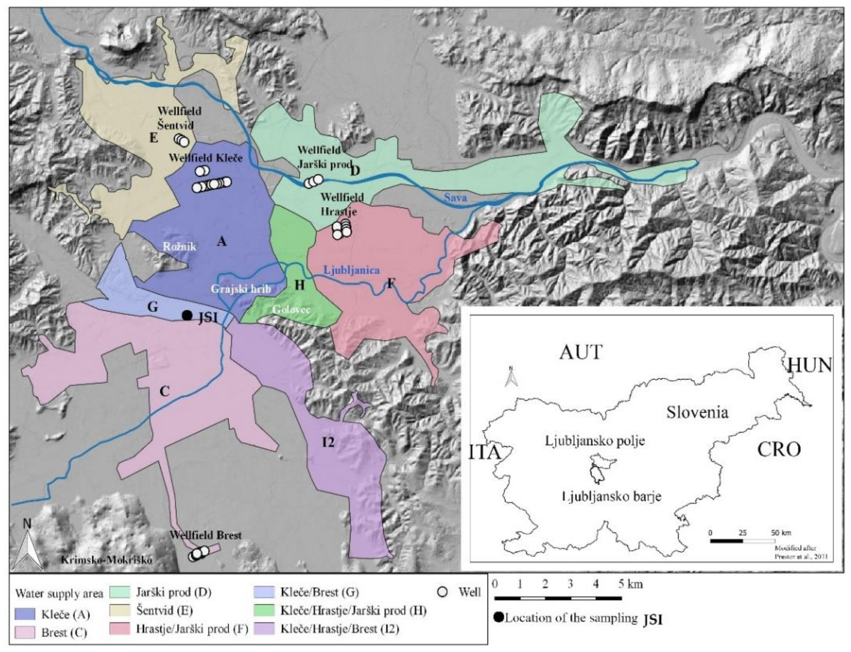
Hourly samples of tap water were collected from the main building’s basement at Jožef Stefan Institute (JSI in Figure 1), Ljubljana, Slovenia (lat: 46.04207, long: 14.487400). The water originates from two different wellfields: Kleče and Brest (Figure 1), located in aquifers with different hydrogeological characteristics. Kleče is located in the Ljubljansko polje aquifer and Brest on the Ljubljansko barje aquifer. Two rivers bind the Ljubljansko polje: the River Ljubljanica to the south and the River Sava to the north in the eastern part of the Ljubljana basin. The basin was formed by tectonic subsidence in the early Pleistocene and is composed of Permian and Carboniferous slate claystone and sandstone [28]. The Pleistocene and Holocene fluvial sediments, accumulated by the River Sava, form highly permeable partially cemented sand and gravel with lenses of conglomerate [29]. The aquifer is recharged by both precipitation and the River Sava, mainly in the north-western part. It is also recharged via lateral inflow from the Ljubljansko barje multi-aquifer system in the south [30,31].
The depression of the Ljubljansko barje is located on the southern part of the Ljubljansko polje; it formed within the permeable limestone and dolomite basement and was filled by alluvial, marshy, and lacustrine sediments during the Pleistocene and Holocene. The upper Holocene aquifers are recharged directly from precipitation and surface streams, while the lower aquifer is recharged from the karst recharge area [32]. Sediments in this area are heterogeneous, and the hydrogeological conditions are more complex than on the Ljubljansko polje [33].
The Ljubljana WSS consists of water supply facilities, 44 wells, eight minor pumping stations, and more than 1100 km of supply network [34]. Groundwater is exploited at the Ljubljansko polje from the Kleče, Hrastje, Jarški prod and Šentvid wellfields and at Ljubljansko barje from the Brest wellfield (Figure 1). In the central system, some settlements are continuously supplied with drinking water from a single wellfield (A, C, D, and E), while others are supplied from two or more wellfields (F, G, H, and I2) [33].
2.2. In-Situ Measurements and Water Sampling
Monitoring of tap water was performed from 09:00 on 24 April 2019 until 09:00 on 25 April 2019. In-situ temperature (T), electrical conductivity (EC), and pH were measured every full hour, using a Hanna HI 9829 Multiparameter instrument (Woonsocket, RI, USA), with an accuracy of ±0.15 °C, ±1 μS/cm and ±0.02, respectively. Quick calibration of the instrument was performed after 4 h, at 13:10.
Before collecting the first sample, the tap water was allowed to run for 60 s. Samples were then collected every hour. In total, 25 water samples were collected. The samples for δ2H and δ18O analysis were stored in prewashed 30 mL high-density polyethylene (HDPE) bottles and stored at room temperature. Samples for δ13CDIC were filtered on-site through a 0.45 µm nylon filter into 12 mL glass exetainers. In contrast, samples for determining the multi-elemental composition and 87Sr/86Sr ratios were collected in prewashed 50 mL polypropylene (PP) centrifuge tubes and acidified using HNO3 (68% v/v, suprapur, Carlo Erba Reagents, Val de Reuil, France). All samples were stored at 4–6 °C.
2.3. Analytical Procedures
The δ2H, δ18O, δ13CDIC, 87Sr/86Sr isotope ratios and major and trace element concentrations were determined at the Department of Environmental Sciences at Jožef Stefan Institute.
2.3.1. Determination of δ2H, δ18O and d-Excess
δ2H and δ18O were determined according to the modified IAEA Technical procedure note no. 43 [35], using the H2-H2O [36] and CO2-H2O [37,38] equilibration techniques. Measurements were performed on a dual inlet isotope ratio mass spectrometer (DI IRMS, Finnigan MAT DELTA plus Finnigan MAT GmbH, Bremen, Germany) with an automated H2-H2O and CO2-H2O equilibrator HDOeq 48 Equilibration Unit (custom built by M. Jaklitsch). The water bath was set to 18 °C. The water vapor trap was cooled to –55 °C. H2 (IAEA) and CO2 (Messer 4.5) gases were used as working standards. Samples (3 mL) were allowed to equilibrate for 2 (H2-H2O) and 6 (CO2-H2O) hours before analysis.
All measurements were performed together with laboratory reference materials (LRM) calibrated periodically against primary IAEA calibration standards to the VSMOW/SLAP scale. The defined isotope values and measurement uncertainty of LRMs were used to normalize the data, and independent quality control was calculated using the Kragten method [39,40,41]. All samples were measured in duplicate. The results were normalized to VSMOW/SLAP using LIMS (Laboratory Information Management System for Light Stable Isotopes) program and expressed in the standard δ notation (in ‰) using the conventional delta notation:
δsample(‰) = (Rsample/Rstandard − 1) × 1000
Rsample and Rstandard are the isotope ratios (2H/1H, 18O/16O) of a heavy isotope to a light isotope in a sample and an international standard. For normalization, the method uses LRMs calibrated to the VSMOW/SLAP scale, namely W-3869 with defined isotope values and estimated measurement uncertainty δ2H = +2.5 ± 0.7‰ and δ 18O = +0.36 ± 0.04‰, and W-3871 with values of δ2H = −148.1 ± 0.7‰ and δ18O = −19.73 ± 0.02‰. LRM W-45 with defined isotope values and estimated measurement uncertainty of δ2H = −60.6 ± 0.7‰ and δ18O = −9.12 ± 0.04‰, and commercial reference materials USGS 45, USGS 46, and USGS 47 were used. The average sample repeatability for δ2H 0.2‰ and δ18O was 0.01‰. Deuterium excess (d) was calculated as d [‰] = δ2H − 8 × δ18O [42].
2.3.2. Determination of δ13CDIC
δ13CDIC was determined according to modified [43] and [44] methods. Saturated phosphoric acid (100%) was added (100–200 µL) to a septum-sealed tube and purged with pure He. A water sample (1 mL) was then injected into the tube, and the isotope composition of CO2 measured directly from the headspace using a continuous flow IsoPrime100 stable isotope mass spectrometer (CF IRMS) coupled with the MultiFlow Bio equilibration unit. The results were normalized to VPDB and expressed in the standard δ notation in ‰ (see Section 2.3.1). A standard solution of Na2CO3 (Carlo Erba reagents, Val de Reuil, France) with a known δ13CDIC of –10.8 ± 0.2‰ was used to determine the optimal extraction procedure for tap water samples. The average sample repeatability was 0.1‰.
2.3.3. Determination of Major and Trace Elements
Four major (Ca, Na, K, Mg) and 23 trace elements concentrations (Ag, Al, As, B, Ba, Cd, Co, Cr, Cu, Fe, K, Li, Mn, Mo, Ni, Pb, Rb, Sb, Se, Sr, U, V, and Zn) were determined using an Agilent 7900x inductively coupled plasma mass spectrometer (ICP-MS, Agilent Technologies, Tokyo, Japan). To measure accuracy, two surface water reference materials: SLRS-5 (National Research Council Canada, Ottawa, ON, Canada) and SPS-SW1 (Spectrapure Standards, Manglerud, Norway), were analysed at the beginning, in the middle and at the end of the sequence. Recovery ranged from 97% to 102% for all elements, and the repeatability was better than 5%.
2.3.4. Determination of 87Sr/86Sr Isotope Ratios
Five samples were selected for 87Sr/86Sr isotope ratio analysis according to the Sr and Rb concentrations and their ratio (10:00, 17:00, 00:00, 03:00 and 08:00). The 87Sr/86Sr isotope ratio was determined using the method described in Zuliani et al. [12]. Briefly, water samples (from 0.1 to 1 mL) were evaporated to dryness and redissolved in 1 ml of 8M HNO3. For Rb/Sr separation, Sr specific resin (Eichrom®, Triskem International, Bruz, France) was used. The 87Sr/86Sr isotope ratio was determined using a Nu plasma II multi-collector ICP-MS (Nu Instruments Ltd., Wrexham, UK) fitted with an Aridus II™ Desolvating Nebulizer System (Teledyne Cetac, Omaha, NE, USA). Measurements were performed following the standard-sample-standard bracketing method using a NIST SRM 987 SrCO3 (0.71034 ± 0.00026, National Institute of Standards and Technology, Gaithersburg, MD, USA) as the standard. All samples were prepared in triplicate.
2.3.5. Data Evaluation
Metadata information is explained in Supplementary Table S1, and all data obtained are presented in Tables S2 and S3. Since the Ag content in most samples and Se in all samples (Table S3) were below the LOD, they were excluded from further data analysis. The data were analyzed using Microsoft® office Excel 2019 for basic descriptive statistics and OriginPro 2021 for multivariate analysis: Spearman correlation coefficient analysis (SCA), hierarchical cluster analysis (HCA), and principal components analysis (PCA). The HCA method was used to order data and create groups that share common properties. Euclidean distances were chosen as the distance between the different sampling times, and Ward’s method was used to form the clusters.
Finally, the simple linear mixing model (SLMM) was used to quantify the relative contribution from each well (Kleče and Brest), using the long-term average concentrations of sodium (Na), chromium (Cr), and arsenic (As) in the two end-members as follows:
NaJSI = xKNaK + yBNaB
1 = xK + yB
Here, the subscript JSI, K and B represent tap water mixture at the JSI and the two water sources Kleče and Brest. For the end-member concentration, long-term data collected at private households at the Kleče and Brest wellfield were used as no simultaneous sampling of source water was provided [45].
3. Results and discussion
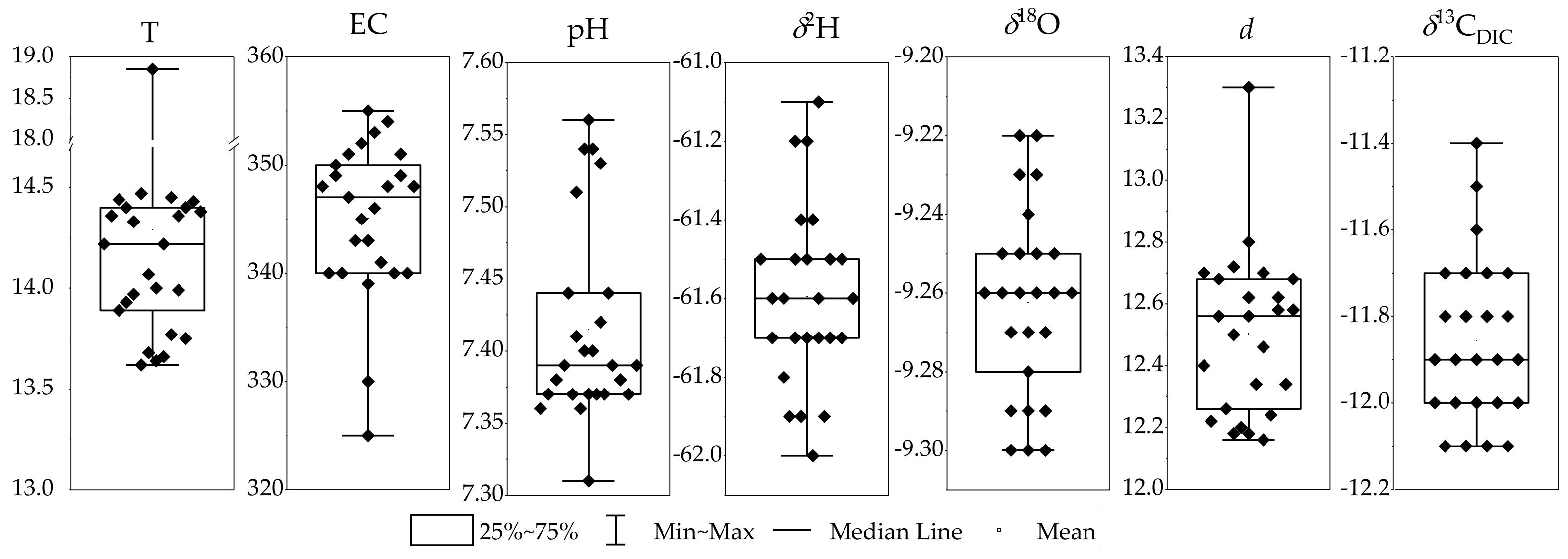
The results are presented as electronic supplementary material (Tables S2 and S3) and summarized graphically in Figure 2 and Figure 3. The descriptive statistics of all hydrogeochemical parameters are presented in Table 1.
Differences observed over the 24 h sampling period were relatively small (Table 1), but a more detailed inspection reveals variations in particular parameters. For instance, after stabilization, the temperature varied between 13.5 °C to 14.5 °C, however the initial reading after one minute was 18.9 °C. The pH ranged from 7.10 to 7.61 (Table 1) and is in the range required for drinking water in Slovenia, i.e., between ≥6.5 and ≤9.5 [20], which is similar to the European standards [21,46] (Table 1). The EC values were between 325 µS/cm and 355 µS/cm and were below the official standard for drinking water of 2500 µS/cm (Table 1). Based on EC classification [48], tap water at the JSI sampled has a low mineral concentration and is homogenous.
3.1. δ2H and δ18O in the Tap Water
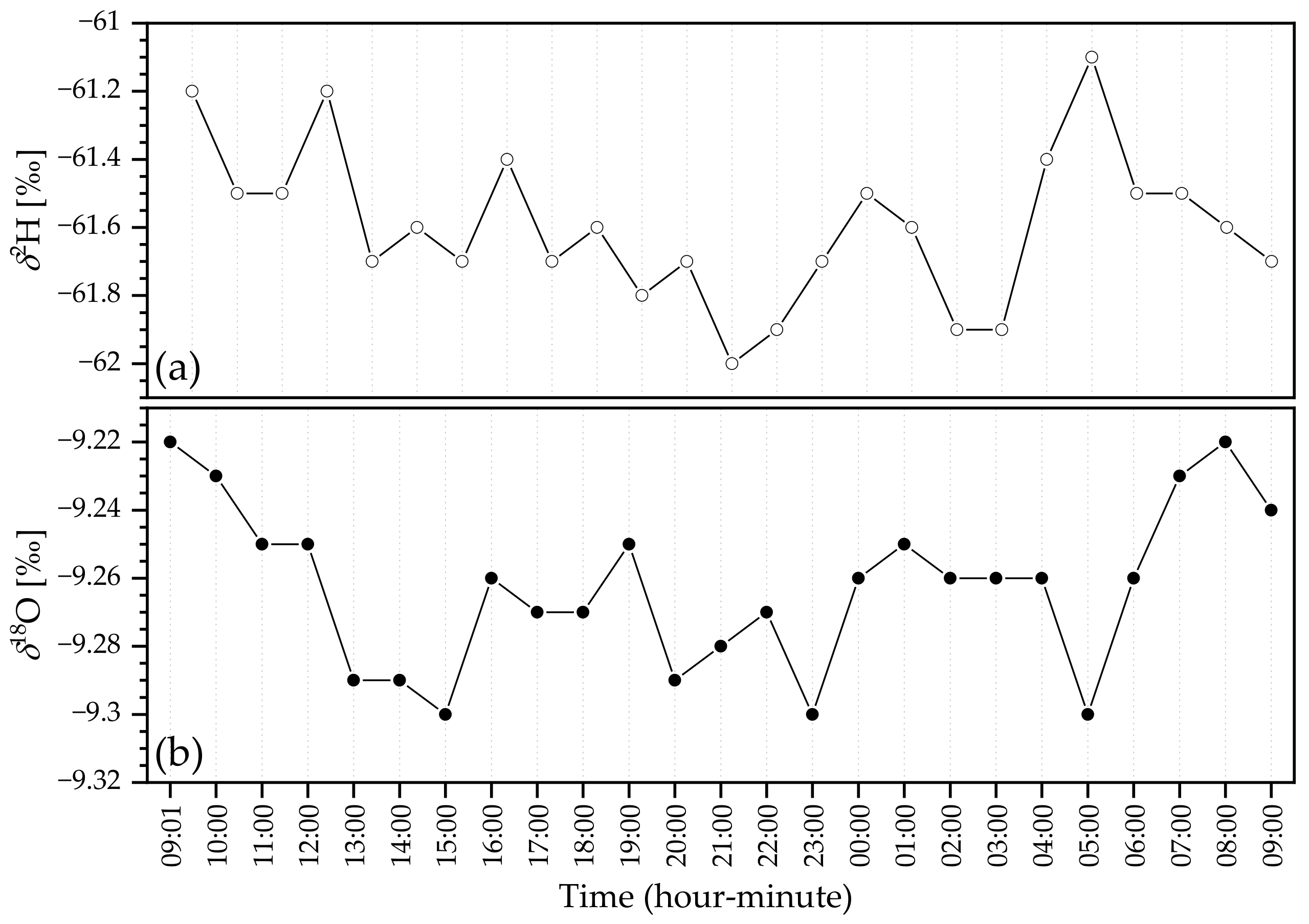
The diurnal variations of stable isotope ratios in tap water are presented in Figure 4 and, as a whole, show only slight statistically nonsignificant variations. The δ2H and δ18O vary from −62.0‰ to −61.1‰ and from −9.30‰ to −9.26‰ (Table 1), respectively, standard deviations for hourly δ2H and δ18O are 0.2‰ and 0.02‰, respectively. The highest and the lowest δ2H appeared at 05:00 and 21:00 (Figure 4a). The highest δ18O appeared at 09:01 and 08:00, and the lowest at 15:00, 23:00, and 05:00 (Figure 4b). Also, there was no significant difference between the average values in tap water during the day-time (09:01–20:00) and night-time (21:00–09:00) [49]. However, there is a slight difference between the average isotope values during morning hours (09:01–11:00 and 07:00–09:00) and the rest of the day/night time (12:00–06:00). The difference for δ2H and δ18O is 0.13‰ and 0.04‰. However, the variability is still small and is in the range of measurement uncertainty. It also shows that the sources of tap water from Kleče and Brest have similar isotope compositions, which prevents the differentiation of tap water origin solely using stable isotope ratios (Figure 4).
No correlation (r = 0.3) was observed between δ2H and δ18O since the source water does not change in such a short period (24 h). Moreover, as the water moves through the soil, the groundwater signal is attenuated resulting in small differences between aquifers. The values obtained are typical for the source water, i.e., groundwater from shallow aquifers of Ljubljansko polje and Ljubljansko barje [25].
All values fall close to the Global Meteoric Water Line (GMWL) and the Local Meteoric Water Line for Ljubljana [50], confirming that groundwater from the Ljubljansko polje aquifer originates primarily from infiltration of local precipitation and water from the River Sava [18] and at the Ljubljansko barje aquifer from precipitation and surface streams [33]. Deuterium excess (d) was also relatively constant, with an average of 12.5‰, and ranging between 12.2‰ and 13.3‰. Therefore, it could not be used as an indicator of different water sources.
3.2. δ13CDIC in the Tap Water
The 24 h δ13C variability of tap water ranged from −12.1‰ to −11.4‰ (Table 1). The lowest δ13CDIC of −12.1‰ was observed at 14:00, 15:00, 17:00, and 3:00, while the highest value of −11.4‰ occurred at 08:00. Samples with lower δ13CDIC are more characteristic for Brest, while samples with higher δ13CDIC are characteristic for Kleče [26]. All values in tap water indicate both biogeochemical processes: CO2 produced during organic matter decomposition and carbonate dissolution.
3.3. Concentrations of Major and Trace Elements in the Tap Water
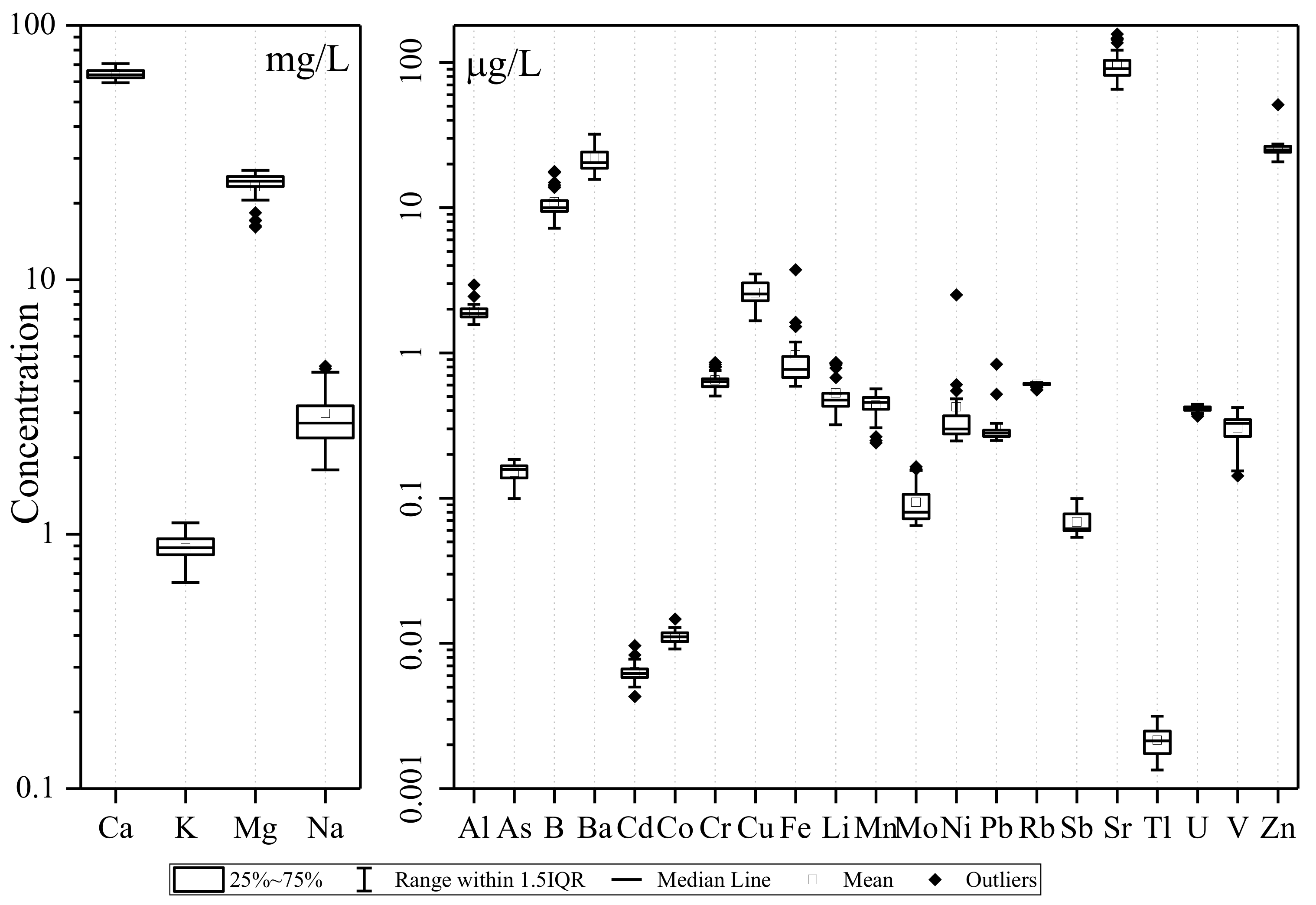
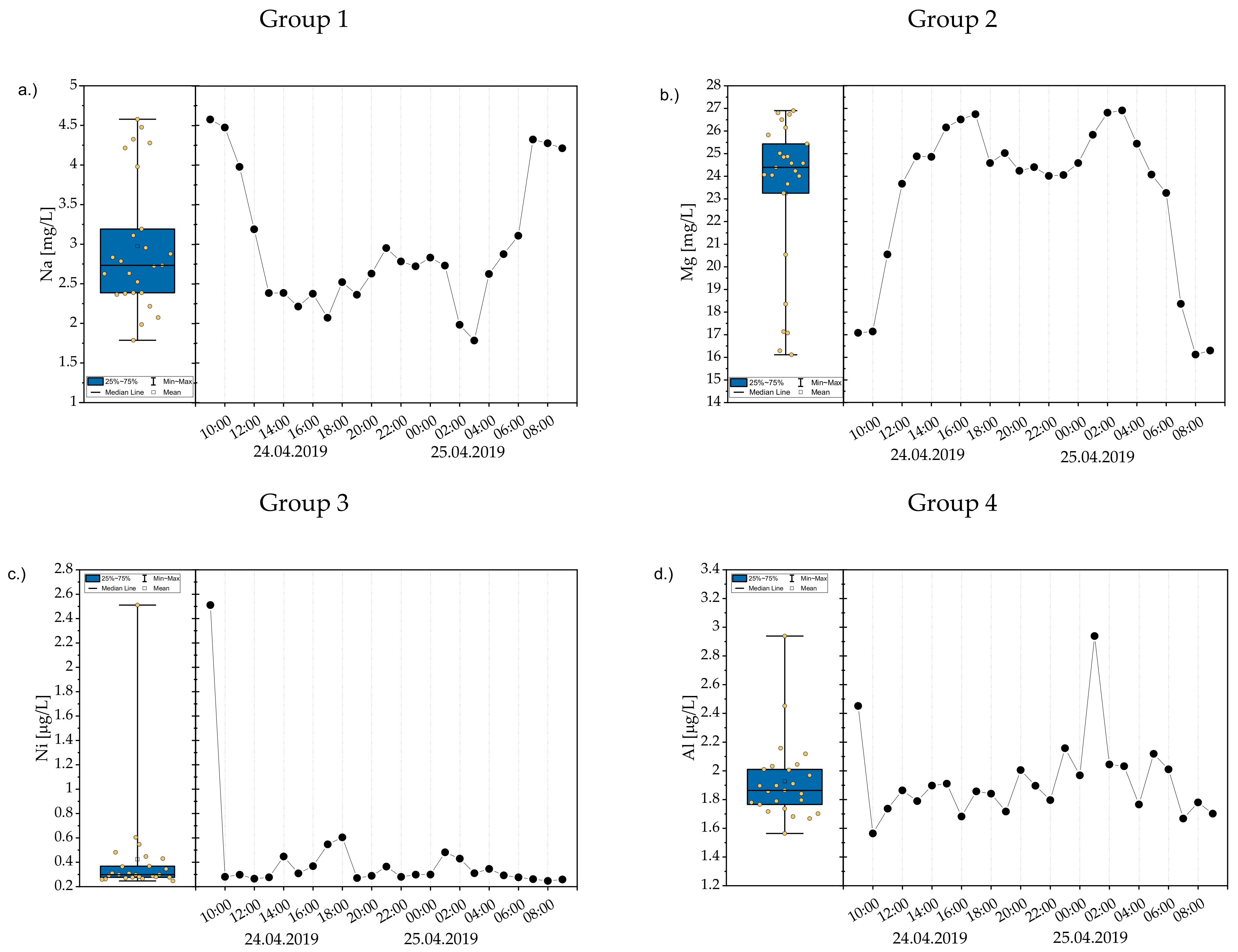
The largest variation in major elements was observed for Na (CV = 28.1%; Figure 5a) followed by K (CV = 14.2%) and Mg (15.0%; Figure 5b) (Table 1). Generally, higher values were observed for Ca and Na at the beginning and at the end of the experiment and opposite for Mg and K that had lower values at the start and end of the experiment (Figure 5a,b). However, data for K show much higher fluctuations during the 24 h experiment. There is no numerical Slovenian drinking water quality guideline for Ca, Mg, and K (Table 1). Trace elements were detected in all water samples, but were below the limits set by the Slovenian regulation and the EU Drinking Water Directive [20,21,22,46,47].
Based on the visual examination of the data, we can distinguish four different groups:
- (1)
- Group 1 (Figure 5a): higher values in the beginning and at the end and lower in between (i.e., δ18O, δ13CDIC, Ca, Na, B, Ba, Cr, Li, Sr);
- (2)
- Group 2 (Figure 5b): lower values in the beginning and at the end and higher in between (i.e., K, Mg, As, Mn, V);
- (3)
- Group 3 (Figure 5c): higher values at the beginning of the experiment (i.e., T, Cd, Co, Fe, Ni, Pb, Sb, Zn) with a subgroup showing exponential decrease with time (i.e., Mo, Sb, Tl);
- (4)
- Group 4 (Figure 5d): no specific pattern; (i.e., EC, pH, δ2H, d, Al, Cu, Rb, U).
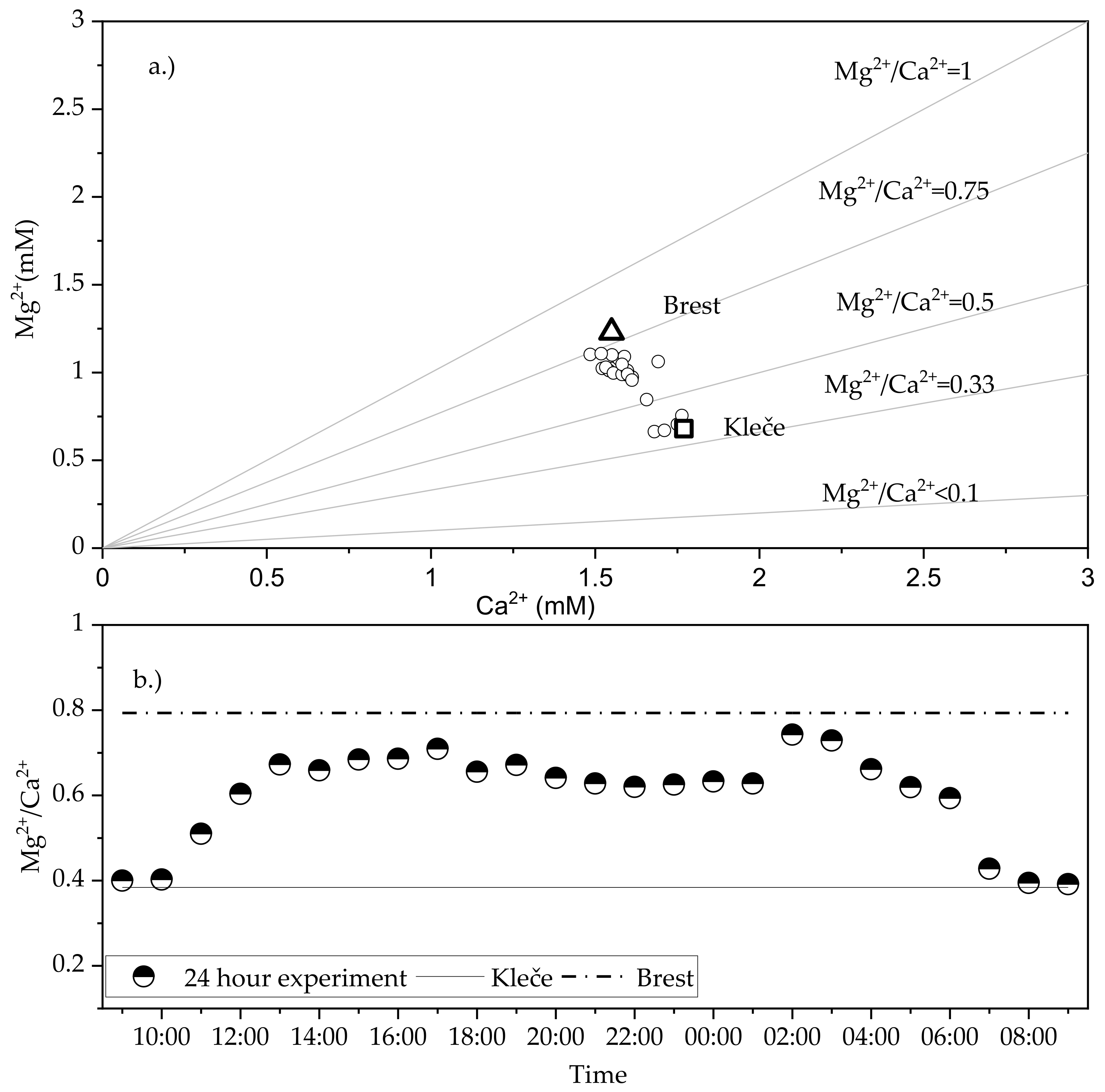
Drinking water in the central WSS has been subject to periodic monitoring of different parameters. In the period 2016 to 2019, measured Ca and Mg concentrations [45] from an average wellfield were 70.8 mg/L (1.77 mM) and 16.5 mg/L (0.68 mM) in Kleče, and 62.0 mg/L (1.55 mM) and 29.7 mg/L (1.23) from the Brest wellfield respectively. The average Mg2+/Ca2+ ratio for Kleče is 0.38 and for Brest 0.79 (Figure 6). Carbonate dissolution plays an important role: in Brest, dolomite dissolution prevails, whereas in Kleče, limestone dissolution is more important. The Mg2+/Ca2+ ratio during the 24 h experiment shows that most samples have a Mg2+/Ca2+ ratio between 0.5 and 0.75, which indicates that the dominant water source is Brest. In contrast, samples below the 0.5 line (09:01, 10:00 and 11:00 on 24 April 19 and 07:00, 08:00 and 09:00 on 25 April 19) suggest that water from Kleče predominates (Figure 6).
3.4. Sr/86Sr Isotope Ratio
The 87Sr/86Sr values are presented in Supplementary Table S3. The Rb concentration in the samples was 0.558 to 0.614 µg/L, with the lowest values at 10:00 and 08:00. The Sr concentration was in the range of 65.2 µg/L to 147 µg/L. The water collected during morning hours (at 10:00 and 08:00) had a lower Rb/Sr ratio than the samples collected at 17:00, 00:00, and 03:00. The hours when the Rb/Sr ratio corresponds to the low Mg2+/Ca2+ ratios (chapter 3.4) allow us to conclude that the samples collected in the morning belong to the water from Kleče, while higher ratios indicate the prevailing water from Brest [27].
3.5. Multivariate Statistical Analysis
The multivariate statistical analysis was performed using SCA, HCA, and PCA. The SCA results are summarized in Supplementary Figure S1, HCA is presented in Figure 7 and Supplementary Table S4, while PCA results are presented in Supplementary Table S5. The final dataset used for multivariate statistical analysis is a data matrix of 25 samples (observations) by 32 parameters (variables) for SCA, while for the PCA and HCA, only 25 parameters, i.e., major and trace elements, were used (Table 1). The distribution of most chemical parameters is positively (Al, B, Ba, Cr, Fe, Li, Mo, Ni, Pb, Sb, Sr, Zn) or negatively (Mg, Mn, As, Rb, V) skewed and only a few are close to a normal distribution (Ca, K, Na, Cd, Co, Cu, Tl, U). Chemical parameters that were positively or negatively skewed were log-transformed. Finally, standardization was applied to 16 lognormal data and 12 normal distributions to ensure that each variable is weighted equally.
Based on the results of the SCA (Figure S1), all the parameters were divided into three groups regarding the number of significant correlations with other parameters:
- (1)
- Parameters with ≤10 correlations (T, EC, d, Al, Co, Cu, Fe, Mo, Pb, Rb, Sb, and Tl);
- (2)
- Parameters with 11 to 19 correlations (pH, δ2H, δ18O, δ13CDIC, Ca, K, As, Li, Ni, and U);
- (3)
- Parameters with 20 and 21 correlations (Mg, Na, B, Ba, Cd, Cr, Mn, Sr, V, and Zn).
δ2H, δ18O, δ13CDIC showed a significant correlation with 12, 15, and 18 other parameters, respectively, and can therefore be used as possible indicators for determining water origin and changes in the WSS. A significant positive Spearman correlation (rs = 0.9) exists between Ca and Na, B, Ba, Cr, Li, and Sr, suggesting a common water origin. It also shows a high negative correlation (rs ≥ −0.7) with As, Mg, Mn, and V, resulting in a possible different origin of the water.
HCA was first performed on the whole set of data (Figure 7a; N = 25), and then on the results after removing the first observation (sample: 09:01; Figure 7b; N = 24). In this study, a horizontal line is drawn across both dendrograms at a linkage distance of about 12. Three distinct clusters were identified: A2 (N = 6), A3 (N = 11), and A4 (N = 7), while cluster A1 (Figure 7a) represents only the first sample. Observation of the dendrogram reveals some similarities between clusters; however, the clusters A1 (only in the left dendrogram) and A2 are less similar as they have high linking similarity clusters A3 and A4. To describe the characteristics of each cluster, Table S4 presents the median values of geochemical data. To the group A1 belongs sample collected at 09:01, to group A2 belong samples collected from 10:00 to 12:00 and from 07:00 to 09:00 and can be attributed to water from Kleče. On contrary, to A3 belong samples collected during the hours when majority of water was coming from Brest (from 13:00 to 20:00 and 01:00 to 03:00). To the group A4 belong samples collected from 21:00 to 00:00 and from 04:00 to 06:00 and represents hours in between the origin change. For cluster A1, we can see that the elevated median values of Fe, Ni, Pb, and Zn indicate the leaching of elements from the WSS collected at the beginning of the experiment and can be linked to the visual classified Group 3. The second dendrogram shows that the clusters include the same tap water samples as in the first dendrogram; however, the representative median concentrations changed (Table S2). The most representative elements for the A2 cluster of the second dendrogram are Ca, Na, B, Ba, Cr, Fe, Li, Mo, Sb, and Sr, while for the A3 cluster, higher values of K, Mg, As, Cd, Co, Ni, Rb, Tl, V, and Zn are characteristic. Most elements (Ca, Na, B, Ba, Cr, Li, and Sr) representative of A2 belongs to Group 1 (Fe, Mo, and Sb belong to Group 3), while elements K, Mg, As, V and Cd, Co, Ni, Tl, Zn belong to visually divided Group 2 and Group 3, respectively (Figure 5b,c). For A4, the most representative elements are Al, Cu, and U that belong to Group 4 (Figure 5d) and confirm the mixing of water, presented in Figure 6.
In 2018, the multi-elemental analysis was performed on water samples from one well in Brest and one well in Kleče. The results showed higher values of B, Ba, Li, and Sr in Kleče, whereas in Brest, higher Mg, As, and V values were detected [27]. Based on all results, we can conclude that the tap water samples in the cluster A2 represent water from Kleče and those in A3 from Brest.
The first two principal components account for 72.7% of the total variance in the dataset; the principal component loadings are presented in Table S5 (left). Loadings that represent the most important variables for the components are bolded for values greater than 0.25. PC1 explains the greatest amount of the variance and is characterized by positive loadings in Ca, Na, B, Ba, Cr, Li, and Sr (Table S5), and belongs to Group 1 (Figure 5a) and can be attributed to the wellfield Kleče. Component 2 is characterized by positive loadings in Al, Cd, Co, Fe, Ni, Pb, and Zn, were all but Al represent Group 3 (Figure 5c).
Further, the first sample was excluded, and the analysis was performed for 24 samples. The results are presented in Table S5 (right). The first two components account for 70.2% of the total variance in the dataset. Component 1 is characterized by positive loadings in Mg, Mn, and V, representing Group 2 (Figure 5b, Table S5), while component 2 is characterized by positive loadings in Mo, Sb, and Tl. The latter elements belong to subgroup 3. The most significant loadings belong to elements related to the leaching from the pipes within the WSS.
3.6. Mixing of Water
Tap water can involve two or more discrete end-members and is easy to observe and calculate. It is important to demonstrate that the tracers of mixing behave conservatively and not react with other solutes, solids, or gases. For the source partitioning, Na was selected for SLMM. Also, Cr and As were used since they represent common contaminants in groundwater [51]. It is known that Ljubljansko polje is higher in Cr, while higher As values are characteristic of Ljubljansko barje. Also, Cr and As are highly correlated with Na and can be used for SLMM. Data of Na concentrations were gathered from 2016 to 2019 in periodical sampling of drinking water [45] with an average value of 4.9 mg/L (min = 3.3 mg/L, max = 7.7 mg/L) for Kleče and 1.6 mg/L (min = 0.99 mg/L, max = 4.4 mg/L) for Brest. By comparing these results with this study’s data, all tap water samples fall in the mixing area between Kleče and Brest. Using equation 2.3.5 and average Na concentration data for end members, the proportion of water from Kleče was calculated. Results show that over 24 h the mixing ratio changed from 7% to 90%. When using Cr and As as end-members and long-term data from private users [45], it gave estimates of 23% to 74% and 0.1% to 100%, respectively. Moreover, based on the high positive correlation between Na and, e.g., Mg, Li, Mn, Sr, and V these elements could also be used for the source determination if the end-member concentration would be known.
4. Conclusions
This study is, to the best of our knowledge, the first to look at the variability of stable isotopes and elemental composition during a 24 h analysis of tap water. It involved in-situ monitoring of T, EC, and pH. Samples were collected for multi-elemental and stable isotope analyses (δ2H, δ18O and δ13CDIC) every hour over 24 h in tap water at a location where water from Kleče and Brest wellfields is mixed.
Using the isotope composition (δ2H, δ18O, and δ13CDIC) to determine the mixing ratios remains inconclusive given the isotope similarity between the two sources waters. Concentrations of elements, although low, did carry more information. Based on the visual observation of temporal differences, four groups were identified. The characteristics of these were: higher values in the beginning and at the end and lower between; lower values in the beginning and at the end and higher in between; higher values at the beginning of the experiment; and a group with no specific pattern. While the isotopes can help us to understand the sources and dynamics of flows in urban areas, the use of additional hydrogeochemical parameter in the SCA, HCA, and PCA analyses helps with testing and identifying hourly variability and the origin of tap water at given time. Based on SCA we divided the investigated parameters into three groups based on the number of significant correlations: parameters that have 10 or less significant correlations (i.e., d), parameters with 11 to 19 significant correlations (i.e., δ18O) and parameters with 20 or 21 significant correlations (i.e., Ca). Stable isotopes are weakly but significantly correlated with different parameters. Considering HCA for all samples collected, samples were linked together based on the time of sampling: the tap water was divided into four clusters (A1, A2, A3, and A4), however when removing the first sample, samples were grouped into three groups (A2, A3, and A4). The cluster A1 (also part of the third visual observed pattern), indicates the influence of the leaching of specific elements (e.g., Fe, Ni, Pb, Zn), probably due to leaching from the water pipe of the internal WSS at the beginning of the experiment, when drinking water starts flowing. The latter was also confirmed with elevated PCA loadings.
Altogether, the results indicate that, as expected, the proportion of water from Kleče and Brest changed throughout the day. However, since no simultaneous data from the sources were provided, the long-term average concentration of Na was considered for SLMM. The proportion of water from Kleče changed from 7% to 90% over the 24 h experiment. Moreover, Cr and As show similar mixing ratios. The results show that at the beginning and the end of the experiment, a higher proportion of the water was from Kleče, whereas between 12:00 and 18:00, most water was from Brest. It should be emphasized that the water managers know the WSS, namely the exact information of the capacity at which wells operate, measured in 15 min intervals. However, by performing this experiment we confirmed their assumptions about the mixing of water in the investigated area with application of elemental composition of tap water. The results, which positively reflect assumptions, show that during the day, when water consumption is high, Brest wellfield contributes a larger share of water. During the night, the Brest wellfield contribution is low and the Kleče wellfield contribution pushes the watershed between the wellfields to the south of the city.
Within this study we can conclude that elemental composition of some elements (i.e., N and As) could be used to provide good proxies of water mixing from two different reservoirs. We must acknowledge that shallow aquifers are characterized by the hydrometeorological seasonal variability that affects the water chemistry. At the time of the experiment, data on the chemistry of water from wells had not been acquired, and long-term data of regular monitoring was used. Therefore, long-term multi-parameter monitoring should be established to determine the monthly and seasonal variations. Finally, we planned to repeat the experiment under different conditions in WSS (i.e., during different seasons and the COVID-19 pandemic when water consumption has significantly changed due to lockdowns) to deduce parameters that can help in long-term evaluation of mixing water at the tap.
Supplementary Materials
The following are available online at https://www.mdpi.com/article/10.3390/w13111451/s1, Figure S1: Pearson correlation matrix for all the analyzed parameters. * p ≤ 0.005. H, O, and C represents δ2H, δ18O and δ13CDIC, respectively; Table S1: Metadata information regarding data attributes; Table S2: Basic sampling attributes and results of temperature (T), electrical conductivity (EC) and pH for all measurements; Table S3: Elemental compositions of the analyzed tap water samples collected every full hour; Table S4: Geochemical characteristics of median concentrations: left for four clusters and right for three clusters; Table S5: Principal component loadings and explained variance for the two components.
Author Contributions
Conceptualization, K.N. and P.V.; method, K.N. and P.V.; formal analysis, K.N., P.V., T.K., and T.Z.; investigation, K.N., P.V., T.K., T.Z., B.B.Ž. and B.J.; resources, P.V., T.K., T.Z., B.B.Ž. and B.J.; data curation, K.N., P.V., T.K., T.Z., and B.J.; writing—original draft preparation, K.N.; writing—review and editing, K.N., P.V., T.K., T.Z., B.B.Ž. and B.J.; visualization, K.N.; supervision, P.V.; funding acquisition, P.V. All authors have read and agreed to the published version of the manuscript.
Funding
Slovenian Research Agency funded this research—ARRS Programme (P1-0143), Young research program (PR-09780), IAEA CRP—Use of Isotope Techniques for the Evaluation of Water Sources for Domestic Supply in Urban Areas (F33024, No. 22843) and Bilateral Research Project BI-US/19-21-078.
Institutional Review Board Statement
Not applicable.
Informed Consent Statement
Not applicable.
Data Availability Statement
Data is contained within the article or supplementary material.
Acknowledgments
Special thanks are due to S. Žigon for his valuable help with H, O and C isotope analysis.
Conflicts of Interest
The authors declare no conflict of interest.
References
- Salvadore, E.; Bronders, J.; Batelaan, O. Hydrological modelling of urbanized catchments: A review and future directions. J. Hydrol. 2015, 529, 62–81. [Google Scholar] [CrossRef]
- Schnoor, J.L. Recognizing Drinking Water Pipes as Community Health Hazards. J. Chem. Educ. 2016, 93, 581–582. [Google Scholar] [CrossRef] [PubMed] [Green Version]
- Schirmer, M.; Leschik, S.; Musolff, A. Current research in urban hydrogeology—A review. Adv. Water Resour. 2013, 51, 280–291. [Google Scholar] [CrossRef]
- Jameel, Y.; Brewer, S.; Fiorella, R.P.; Tipple, B.J.; Terry, S.; Bowen, G.J. Isotopic reconnaissance of urban water supply system dynamics. Hydrol. Earth Syst. Sci. 2018, 22, 6109–6125. [Google Scholar] [CrossRef] [Green Version]
- Bowen, G.J.; Cai, Z.; Fiorella, R.P.; Putman, A.L. Isotopes in the Water Cycle: Regional- to Global-Scale Patterns and Applications. Annu. Rev. Earth Planet. Sci. 2019, 47, 453–479. [Google Scholar] [CrossRef] [Green Version]
- Zhao, S.; Hu, H.; Tian, F.; Tie, Q.; Wang, L.; Liu, Y.; Shi, C. Divergence of stable isotopes in tap water across China. Sci. Rep. 2017, 7, 43653. [Google Scholar] [CrossRef] [Green Version]
- De Wet, R.F.; West, A.G.; Harris, C. Seasonal variation in tap water δ2H and δ18O isotopes reveals two tap water worlds. Sci. Rep. 2020, 10, 13544. [Google Scholar] [CrossRef]
- Atekwana, E.; Krishnamurthy, R. Seasonal variations of dissolved inorganic carbon and δ13C of surface waters: Application of a modified gas evolution technique. J. Hydrol. 1998, 205, 265–278. [Google Scholar] [CrossRef]
- Verbovšek, T.; Kanduč, T. Isotope Geochemistry of Groundwater from Fractured Dolomite Aquifers in Central Slovenia. Aquat. Geochem. 2016, 22, 131–151. [Google Scholar] [CrossRef]
- Cartwright, I.; Weaver, T.; Tweed, S.; Ahearne, D.; Cooper, M.; Czapnik, C.; Tranter, J. O, H, C isotope geochemistry of carbonated mineral springs in central Victoria, Australia: Sources of gas and water–rock interaction during dying basaltic volcanism. J. Geochem. Explor. 2000, 69–70, 257–261. [Google Scholar] [CrossRef]
- Ettayfi, N.; Bouchaou, L.; Michelot, J.L.; Tagma, T.; Warner, N.; Boutaleb, S.; Massault, M.; Lgourna, Z.; Vengosh, A. Geochemical and isotopic (oxygen, hydrogen, carbon, strontium) constraints for the origin, salinity, and residence time of groundwater from a carbonate aquifer in the Western Anti-Atlas Mountains, Morocco. J. Hydrol. 2012, 438–439, 97–111. [Google Scholar] [CrossRef]
- Zuliani, T.; Kanduč, T.; Novak, R.; Vreča, P. Characterization of Bottled Waters by Multielemental Analysis, Stable and Radiogenic Isotopes. Water 2020, 12, 2454. [Google Scholar] [CrossRef]
- Chesson, L.A.; Tipple, B.J.; Mackey, G.N.; Hynek, S.A.; Fernandez, D.P.; Ehleringer, J.R. Strontium isotopes in tap water from the coterminous USA. Ecosphere 2012, 3, 67. [Google Scholar] [CrossRef]
- Cloutier, V.; Lefebvre, R.; Therrien, R.; Savard, M.M. Multivariate statistical analysis of geochemical data as indicative of the hydrogeochemical evolution of groundwater in a sedimentary rock aquifer system. J. Hydrol. 2008, 353, 294–313. [Google Scholar] [CrossRef]
- Jameel, Y.; Brewer, S.; Good, S.P.; Tipple, B.J.; Ehleringer, J.R.; Bowen, G.J. Tap water isotope ratios reflect urban water system structure and dynamics across a semiarid metropolitan area. Water Resour. Res. 2016, 52, 5891–5910. [Google Scholar] [CrossRef] [Green Version]
- Du, M.; Zhang, M.; Wang, S.; Chen, F.; Zhao, P.; Zhou, S.; Zhang, Y. Stable Isotope Ratios in Tap Water of a Riverside City in a Semi-Arid Climate: An Application to Water Source Determination. Water 2019, 11, 1441. [Google Scholar] [CrossRef] [Green Version]
- US Environmental Protection Agency. Effects of Water Age on Distribution System Water Quality; EPA: Washington, DC, USA, 2002. [Google Scholar]
- Vrzel, J.; Solomon, D.K.; Željko, B.; Ogrinc, N. The study of the interactions between groundwater and Sava River water in the Ljubljansko polje aquifer system (Slovenia). J. Hydrol. 2018, 556, 384–396. [Google Scholar] [CrossRef]
- Brilly, M.; Jamnik, B.; Drobne, D. Chromium and Atrazine Contamination of The Ljubljansko Polje Aquifer. In Dangerous Pollutants (Xenobiotics) in Urban Water Cycle; NATO Science for Peace and Security Series; Hlavinek, P., Bonacci, O., Marsalek, J., Mahrikova, I., Eds.; Springer: Dordrecht, The Netherlands, 2008; pp. 207–216. ISBN 978-1-4020-6800-3. [Google Scholar]
- Republic of Slovenia, Ministry of Health. Drinking Water Regulations of 1 March 2004; Official Gazette of the Republic Slovenia: Ljubljana, Slovenia, 2004; Volume 19. [Google Scholar]
- European Parliament; Council of the European Union. Directive EU 2020/2184 of the European Parliament and of the Council of 16 December 2020 on the Quality of Water Intended for Human Consumption; Official Journal of the European Communities: Brussels, Belgium, 2020; pp. 1–62. [Google Scholar]
- Mohod, C.V.; Dhote, J. Review of heavy metals in drinking water and their effect on human health. Int. J. Innov. Res. Sci. Eng. Technol. 2013, 2, 5. [Google Scholar]
- Prestor, J.; Jamnik, B.; Pestotnik, S.; Meglič, P.; Cerar, S.; Janža, M.; Auersperger, P.; Bračič-Železnik, B. Upravljanje Onesnaženj Podzemne Vode Na Ravni Funkcionalnega Mestnega Območja. In Proceedings of the Zbornik referatov: Simpozij z mednarodno udeležbo, Ljubljana, Slovenia, 5–6 October 2017; CERKVENIK, Stanka (ur.); ROJNIK, Enisa (ur.): Portorož, Slovenia, 2017; pp. 123–134. [Google Scholar]
- Janža, M.; Prestor, J.; Pestotnik, S.; Jamnik, B. Nitrogen Mass Balance and Pressure Impact Model Applied to an Urban Aquifer. Water 2020, 12, 1171. [Google Scholar] [CrossRef] [Green Version]
- Nagode, K.; Kanduč, T.; Lojen, S.; Železnik, B.B.; Jamnik, B.; Vreča, P. Synthesis of past isotope hydrology investigations in the area of Ljubljana, Slovenia. Geologja 2020, 63, 251–270. [Google Scholar] [CrossRef]
- Vreča, P.; Kanduč, T.; Šlejkovec, Z.; Žigon, S.; Nagode, K.; Močnik, N.; Bračič-Železnik, B.; Jamnik, B.; Žitnik, M. Karakterizacija vodnih virov za javno oskrbo s pitno vodo v Ljubljani s pomočjo različnih geokemičnih analiz. In Raziskave s Področja Geodezije in Geofizike 2018; Kuhar, M., Pavlovčič Prešeren, P., Vreča, P., Eds.; Slovensko združenje za geodezijo in geofiziko: Ljubljana, Slovenia, 2019; pp. 111–119. ISBN 978-961-6884-69-3. [Google Scholar]
- Vreča, P.; Nagode, K.; Zuliani, T.; Lojen, S.; Kanduč, T.; Žigon, S.; Novak, R.; BračičŽeleznik, B.; Jamnik, B.; Žitnik, M. Second Working Report on Multi-Isotope Characterization of Water Resources for Domestic Supply in Ljubljana, Slovenia; Jožef Stefan Institute, Department of Environmental Sciences: Ljubljana, Slovenia, 2019. [Google Scholar]
- Jamnik, B.; Železnik, B.B.; Urbanc, J. Diffuse Pollution of Water Protection Zones in Ljubljana, Slovenia. In Proceedings of the 7th International Specialized Conference on Diffuse Pollution and Basin Management and 36th Scientific Meeting of the Estuarine and Coastal Sciences Association (ECSA), Dublin, Ireland, 17–22 August 2003; pp. 7-1–7-5. [Google Scholar]
- Žlebnik, L. Pleistocen Kranjskega, Sorskega in Ljubljanskega polja. Geologija 1971, 14, 5–51. [Google Scholar]
- Jamnik, B.; Urbanc, J. Izvor in Kakovost Podzemne Vode Ljubljanskega Polja = Origin and Quality of Groundwater from Ljubljansko Polje. RMZ 2000, 47, 167–178. [Google Scholar]
- Vizintin, G.; Souvent, P.; Veselič, M.; Curk, B.C. Determination of urban groundwater pollution in alluvial aquifer using linked process models considering urban water cycle. J. Hydrol. 2009, 377, 261–273. [Google Scholar] [CrossRef]
- Mencej, Z. The Gravel Fill beneath the Lacustrine Sediments of the Ljubljansko Barje. Geologija 1988, 31, 517–553. [Google Scholar]
- Cerar, S.; Urbanc, J. Carbonate Chemistry and Isotope Characteristics of Groundwater of Ljubljansko Polje and Ljubljansko Barje Aquifers in Slovenia. Sci. World J. 2013, 2013, 1–11. [Google Scholar] [CrossRef]
- Jamnik, B.; Žitnik, M. Letno Poročilo o Skladnosti Pitne Vode na Oskrbovalnih Območjih v Upravljanju Javnega Podjetja Vodovod Kanalizacija Snaga d. o. o. v Letu 2019; Javno Podjetje VODOVOD KANALIZACIJA SNAGA d.o.o.: Ljubljna, Slovenia, 2020; p. 27. [Google Scholar]
- Tanweer, A.; Gröning, M.; Van Duren, M.; Jaklitsch, M.; Pöltenstein, L. TEL Technical Note No. 43 Stable Isotope Internal Laboratory Water Standards: Preparation, Calibration and Storage; International Atomic Energy Agency: Vienna, Austria, 2009. [Google Scholar]
- Coplen, T.B.; Wildman, J.D.; Chen, J. Improvements in the gaseous hydrogen-water equilibration technique for hydrogen isotope-ratio analysis. Anal. Chem. 1991, 63, 910–912. [Google Scholar] [CrossRef]
- Epstein, S.A.; Mayeda, T.K. Variation of O18 content of waters from natural sources. Geochim. Cosmochim. Acta 1953, 4, 213–224. [Google Scholar] [CrossRef]
- Avak, H.; Brand, W.A. The Finning MAT HDO-Equilibration—A Fully Automated H2O/Gas Phase Equilibration System for Hydrogen and Oxygen Isotope Analyses. Thermo Electron. Corp. Appl. News 1995, 11, 1–13. [Google Scholar]
- Carter, J.; Barwick, V. Good Practice Guide for Isotope Ratio Mass Spectrometry. FIRMS. 41, 1st ed.; The Forensic Isotope Ratio Mass Spectrometry (FIRMS) Network: Bristol, UK, 2011; Available online: http://www.forensic-isotopes.org/assets/IRMS%20Guide%20Finalv3.1_Web.pdf (accessed on 10 August 2010)ISBN 978-0-948926-31-0.
- Vreča, P.; Žigon, S. Poročilo o Prvi Kalibraciji Laboratorijskih Referenčnih Materialov za Določanje Izotopske Sestave Vodika in Kisika v Vzorcih vod z Masnim Spektrometrom Finnigan MAT DELTA Plus; IJS-DP-12137; Jožef Stefan Institute, Department of Environmental Sciences: Ljubljana, Slovenia, 2016. [Google Scholar]
- Vreča, P.; Žigon, S. Poročilo o Drugi Kalibraciji Laboratorijskih Referenčnih Materialov Za Določanje Izotopske Sestave Vodika in Kisika v Vzorcih Vod z Masnim Spektrometrom Finnigan MAT DELTA Plus; IJS_DP-12138; Jožef Stefan Institute, Department of Environmental Sciences: Ljubljana, Slovenia, 2016. [Google Scholar]
- Dansgaard, W. Stable isotopes in precipitation. Tellus 1964, 16, 436–468. [Google Scholar] [CrossRef]
- Miyajima, T.; Hanba, Y.T.; Yoshii, K.; Koitabashi, T.; Wada, E. Determining the stable isotope ratio of total dissolved inorganic carbon in lake water by GC/C/IIRMS. Limnol. Oceanogr. 1995, 40, 994–1000. [Google Scholar] [CrossRef]
- Spötl, C. A robust and fast method of sampling and analysis of δ13C of dissolved inorganic carbon in ground waters. Isot. Environ. Health Stud. 2005, 41, 217–221. [Google Scholar] [CrossRef]
- Grafični Pregled Rezultatov Občasnih Preskušanj Pitne Vode. Available online: https://www.vokasnaga.si/informacije/kaksno-vodo-pijemo/pregled-obcasnih-preskusanj-pitne-vode-v-prostoru (accessed on 12 November 2020).
- United States Environmental Protection Agency. Ground Water and Drinking Water. Available online: https://www.epa.gov/ground-water-and-drinking-water (accessed on 5 August 2020).
- WHO. Guidelines for Drinking-Water Quality; WHO: Geneva, Switzerland, 2008. [Google Scholar]
- Van Der Aa, M. Classification of mineral water types and comparison with drinking water standards. Environ. Geol. 2003, 44, 554–563. [Google Scholar] [CrossRef] [Green Version]
- Du, M.; Zhang, M.; Wang, S.; Meng, H.; Che, C.; Guo, R. Stable Isotope Reveals Tap Water Source under Different Water Supply Modes in the Eastern Margin of the Qinghai–Tibet Plateau. Water 2019, 11, 2578. [Google Scholar] [CrossRef] [Green Version]
- Vreča, P.; Malenšek, N. Slovenian Network of Isotopes in Precipitation (SLONIP)—A review of activities in the period 1981–2015. Geologija 2016, 59, 67–84. [Google Scholar] [CrossRef]
- Smedley, P.L.; Kinniburgh, D.G. A review of the source, behaviour and distribution of arsenic in natural waters. Appl. Geochem. 2002, 17, 517–568. [Google Scholar] [CrossRef] [Green Version]
Figure 1.
Study area showing the main wellfields (marked with circles) and water supply areas (A to I2). The sampling location is marked with a black dot (JSI).
Figure 1.
Study area showing the main wellfields (marked with circles) and water supply areas (A to I2). The sampling location is marked with a black dot (JSI).

Figure 2.
Boxplots of T [°C], EC [µS/cm], pH, δ2H [‰], δ18O [‰], d [‰], and δ13CDIC [‰] for all tap water samples.
Figure 2.
Boxplots of T [°C], EC [µS/cm], pH, δ2H [‰], δ18O [‰], d [‰], and δ13CDIC [‰] for all tap water samples.

Figure 3.
Boxplots of element concentrations (major and trace elements) in all tap water samples.

Figure 4.
Diurnal variations of stable isotope ratios in tap water: (a) δ2H, (b) δ18O.

Figure 5.
The most representative boxplots and hourly variability of concentrations based on visual observation for Group 1 (a), Group 2 (b), Group 3 (c) and Group 4 (d).
Figure 5.
The most representative boxplots and hourly variability of concentrations based on visual observation for Group 1 (a), Group 2 (b), Group 3 (c) and Group 4 (d).

Figure 6.
(a) Mg2+ versus Ca2+ concentration in tap water samples collected during the 24 h experiment. For comparison, average concentrations for wellfields Kleče (calcite prevails) and Brest (dolomite prevails) are shown. (b) Temporal changes in Mg2+/Ca2+ values in tap water during the 24 h experiment.

Figure 7.
Dendrogram for the tap water samples, showing: (a) the division into four clusters; (b) the division into three clusters.
Figure 7.
Dendrogram for the tap water samples, showing: (a) the division into four clusters; (b) the division into three clusters.


Table 1.
Summary of basic statistics and SI, EU, US EPA, and WHO guidelines for tap water.
| Mean | SD | Min | Max | Range | CV (%) | SI 1 | EU 2 | US EPA 3 | WHO 4 | |
|---|---|---|---|---|---|---|---|---|---|---|
| T [°C] | 14.1 | 0.59 | 13.5 | 18.9 | 5.4 | 7.0 | n.d. | n.d. | n.d. | n.d. |
| EC [µS/cm] | 344 | 7.0 | 325 | 355 | 30 | 2.1 | 2500 | 2500 | n.d. | n.d. |
| pH | 7.43 | 0.09 | 7.10 | 7.61 | 0.51 | 0.9 | 6.5–9.5 | 6.5–9.5 | 6.5–8.5 | n.d. |
| δ2H [‰] | −61.6 | 0.2 | −62.0 | −61.1 | 0.9 | |||||
| δ18O [‰] | −9.26 | 0.02 | −9.30 | −9.22 | 0.08 | |||||
| d [‰] | 12.5 | 0.3 | 12.2 | 13.3 | 1.1 | |||||
| δ13CDIC [‰] | −11.9 | 0.2 | −12.1 | −11.4 | 0.7 | |||||
| Ca [mg/L] | 64.4 | 3.11 | 59.5 | 70.7 | 11.2 | 4.8 | n.d. | n.d. | n.d. | n.d. |
| K [mg/L] | 0.884 | 0.125 | 0.645 | 1.11 | 0.465 | 14.2 | n.d. | n.d. | n.d. | n.d. |
| Mg [mg/L] | 23.3 | 3.48 | 16.1 | 26.9 | 10.8 | 15.0 | n.d. | n.d. | n.d. | n.d. |
| Na [mg/L] | 2.98 | 0.836 | 1.79 | 4.58 | 2.79 | 28.1 | 200 | 200 | n.d. | n.d. |
| Al [µg/L] | 1.93 | 0.283 | 1.56 | 2.94 | 1.38 | 14.7 | 200 | 200 | 50–200 | 100–200 |
| As [µg/L] | 0.150 | 0.025 | 0.099 | 0.184 | 0.085 | 16.4 | 10 | 10 | 10 | 10 |
| B [µg/L] | 10.9 | 2.84 | 7.20 | 17.7 | 10.5 | 26.0 | 1000 | 1000 | n.d. | 2400 |
| Ba [µg/L] | 22.1 | 4.99 | 15.7 | 32.0 | 16.3 | 22.6 | n.d. | n.d. | 2000 | 1300 |
| Cd [µg/L] | 0.0064 | 0.0012 | 0.0043 | 0.0096 | 0.0053 | 18.6 | 5 | 5 | 5 | 3 |
| Co [µg/L] | 0.0111 | 0.0013 | 0.0091 | 0.0147 | 0.0111 | 12.0 | n.d. | n.d. | n.d. | n.d. |
| Cr [µg/L] | 0.651 | 0.096 | 0.504 | 0.859 | 0.355 | 14.7 | 50 | 50 | 100 | 50 |
| Cu [µg/L] | 2.60 | 0.486 | 1.67 | 3.49 | 1.82 | 18.7 | 2000 | 2000 | 1300 | 2000 |
| Fe [µg/L] | 0.970 | 0.631 | 0.588 | 3.73 | 3.14 | 65.1 | 200 | 200 | 300 | n.d. |
| Li [µg/L] | 0.528 | 0.171 | 0.320 | 0.857 | 0.537 | 32.4 | n.d. | n.d. | n.d. | n.d. |
| Mn [µg/L] | 0.437 | 0.093 | 0.240 | 0.566 | 0.326 | 21.3 | 50 | 50 | 50 | n.d. |
| Mo [µg/L] | 0.093 | 0.031 | 0.065 | 0.165 | 0.100 | 33.5 | n.d. | n.d. | n.d. | 70 |
| Ni [µg/L] | 0.424 | 0.445 | 0.247 | 2.51 | 2.26 | 104.8 | 20 | 20 | n.d. | 70 |
| Pb [µg/L] | 0.310 | 0.121 | 0.249 | 0.834 | 0.585 | 39.0 | 10 | 10 | 15 | 10 |
| Rb [µg/L] | 0.606 | 0.019 | 0.555 | 0.624 | 0.069 | 3.1 | n.d. | n.d. | n.d. | n.d. |
| Sb [µg/L] | 0.068 | 0.014 | 0.054 | 0.099 | 0.045 | 20.2 | 5 | 5 | 6 | 20 |
| Sr [µg/L] | 98.1 | 27.2 | 65.2 | 157 | 91.8 | 27.7 | n.d. | n.d. | n.d. | n.d. |
| Tl [µg/L] | 0.0021 | 0.0005 | 0.0013 | 0.0031 | 0.0018 | 22.7 | n.d. | n.d. | 2 | n.d. |
| U [µg/L] | 0.411 | 0.017 | 0.367 | 0.442 | 0.075 | 4.0 | n.d. | n.d. | n.d. | 30 |
| V [µg/L] | 0.301 | 0.079 | 0.142 | 0.420 | 0.278 | 26.4 | n.d. | n.d. | n.d. | n.d. |
| Zn [µg/L] | 25.7 | 5.61 | 20.7 | 51.1 | 30.4 | 21.8 | n.d. | n.d. | 5000 | n.d. |
Publisher’s Note: MDPI stays neutral with regard to jurisdictional claims in published maps and institutional affiliations. |
© 2021 by the authors. Licensee MDPI, Basel, Switzerland. This article is an open access article distributed under the terms and conditions of the Creative Commons Attribution (CC BY) license (https://creativecommons.org/licenses/by/4.0/).
Share and Cite
MDPI and ACS Style
Nagode, K.; Kanduč, T.; Zuliani, T.; Bračič Železnik, B.; Jamnik, B.; Vreča, P. Daily Fluctuations in the Isotope and Elemental Composition of Tap Water in Ljubljana, Slovenia. Water 2021, 13, 1451. https://doi.org/10.3390/w13111451
AMA Style
Nagode K, Kanduč T, Zuliani T, Bračič Železnik B, Jamnik B, Vreča P. Daily Fluctuations in the Isotope and Elemental Composition of Tap Water in Ljubljana, Slovenia. Water. 2021; 13(11):1451. https://doi.org/10.3390/w13111451
Chicago/Turabian StyleNagode, Klara, Tjaša Kanduč, Tea Zuliani, Branka Bračič Železnik, Brigita Jamnik, and Polona Vreča. 2021. "Daily Fluctuations in the Isotope and Elemental Composition of Tap Water in Ljubljana, Slovenia" Water 13, no. 11: 1451. https://doi.org/10.3390/w13111451
Note that from the first issue of 2016, this journal uses article numbers instead of page numbers. See further details here.