Derivation of S-Curve from Oscillatory Hydrograph Using Digital Filter

Abstract

An oscillatory S-curve causes unexpected fluctuations in a unit hydrograph (UH) of desired duration or an instantaneous UH (IUH) that may affect the constraints for hydrologic stability. On the other hand, the Savitzky–Golay smoothing and differentiation filter (SG filter) is a digital filter known to smooth data without distorting the signal tendency. The present study proposes a method based on the SG filter to cope with oscillatory S-curves. Compared to previous conventional methods, the application of the SG filter to an S-curve was shown to drastically reduce the oscillation problems on the UH and IUH. In this method, the SG filter parameters are selected to give the minimum influence on smoothing and differentiation. Based on runoff reproduction results and performance criteria, it appears that the SG filter performed both smoothing and differentiation without the remarkable variation of hydrograph properties such as peak or time-to peak. The IUH, UH, and S-curve were estimated using storm data from two watersheds. The reproduced runoffs showed high levels of model performance criteria. In addition, the analyses of two other watersheds revealed that small watershed areas may experience scale problems. The proposed method is believed to be valuable when error-prone data are involved in analyzing the linear rainfall–runoff relationship.

1. Introduction

Despite its very long history, the S-curve concept is still an integral part of linear system-based hydrology. The S-curve stands for a direct runoff caused by the effective rainfall (ER) applied over an infinite time, and its intensity is one-unit depth per unit of time (e.g., 1 cm h⁻¹). The S-curve is mainly used to alter a unit hydrograph (UH) of specified duration into a UH of desired duration. The S-curve is the integral of an instantaneous unit hydrograph (IUH) produced from a unit impulse rainfall so that the IUH is the first derivative of the S-curve. Therefore, the slope of the S-curve at a particular time is proportional to the IUH ordinate at that time.

The general procedure to generate S-curves is the addition of a series of UHs of specified duration, where each UH is translated by its duration time. The UH for generating the S-curve is usually obtained by solving an inverse problem with respect to a rainfall–runoff relationship. The ordinary least-square (OLS) method is one popular method that deals with UH derivation. However, OLS often causes a situation in which the derived UH exhibits oscillation among its ordinates [1]. This happens when minimizing errors with the least square method results in the original rainfall matrix changing into a resolvable form. The so-determined UH often needs to be adjusted by smoothing to ensure the stability of the hydrological system [2]. Other techniques such as the ridge least-square and optimization methods were developed to overcome oscillation problems, but they are either complex or subjective when determining smoothing parameters [3].

Recently, an alternative approach proposed the use of an analytic function to represent the S-curve and a parametric form of the UH as a kernel of convolution [4]. The authors showed that the analytic S-curve produced runoff similarly accurate to that obtained by conventional methods. A subsequent reinvestigation demonstrated that the analytic S-curve outperformed the method of the Central Water Commission of India [5]. However, this approach needs to consider the influence of the ordinates of an S-curve developed from an oscillatory UH on the fitting parameters of the analytic S-curve. In addition, there are situations where UHs deviate from simple functions [6], which stresses the need to produce more UH-shape-dependent S-curves. Hence, a nonparametric approach can be an alternative because it can cope with unusual situations such as an oscillatory or multi-modal UH, as well as irregular outflow from different catchment shapes.

Theoretically, an IUH can be obtained by directly differentiating the S-curve, but, in practice, it is common to use other methods like harmonic series, Fourier transform, Laplace transform, and conceptual models [7] because of the magnification of the oscillation of the IUH during the differentiation of the S-curve. Attempts were also made to use parametric formulation to derive the IUH from the S-curve, but the parameters appeared to be highly dependent on the specific basin at hand, which made it hard to provide a general method [4]. There is also Diskin’s method, which is known to use differentials through a polygon composed of several straight-line segments to approximate the IUH [8]. This method provides a good estimation of the IUH but does not directly differentiate the S-curve, which makes the procedure subjective and require a lot of work. In previous studies, practitioners seemed to be reluctant to obtain the IUH by directly differentiating the S-curve when dealing with discrete data with errors. Accordingly, this study proposes a practical method for obtaining the IUH by directly differentiating the S-curve.

For this purpose, this study employed a digital smoothing and differentiation filter, called the Savitzky–Golay smoothing and differentiation filter (SG filter) [9], which enables not only the mitigation of the oscillation problem in S-curves and but also the numerical differentiation of the S-curve by assuming a piecewise continuous function. The proposed method uses efficient matrix computation in contrast to conventional, tedious methods. In addition, this method is more objective because it reduces some ambiguity in deciding the filter parameters.

The proposed method is illustrated using four sets of rainfall–runoff data from published papers [10,11]. The performance of the S-curve and IUH derived by the method using the SG filter was evaluated by the well-known Nash–Sutcliffe criterion. The proposed method was found to offer the advantages of being technically simple to perform and timesaving in calculation.

2. Theory

2.1. Method

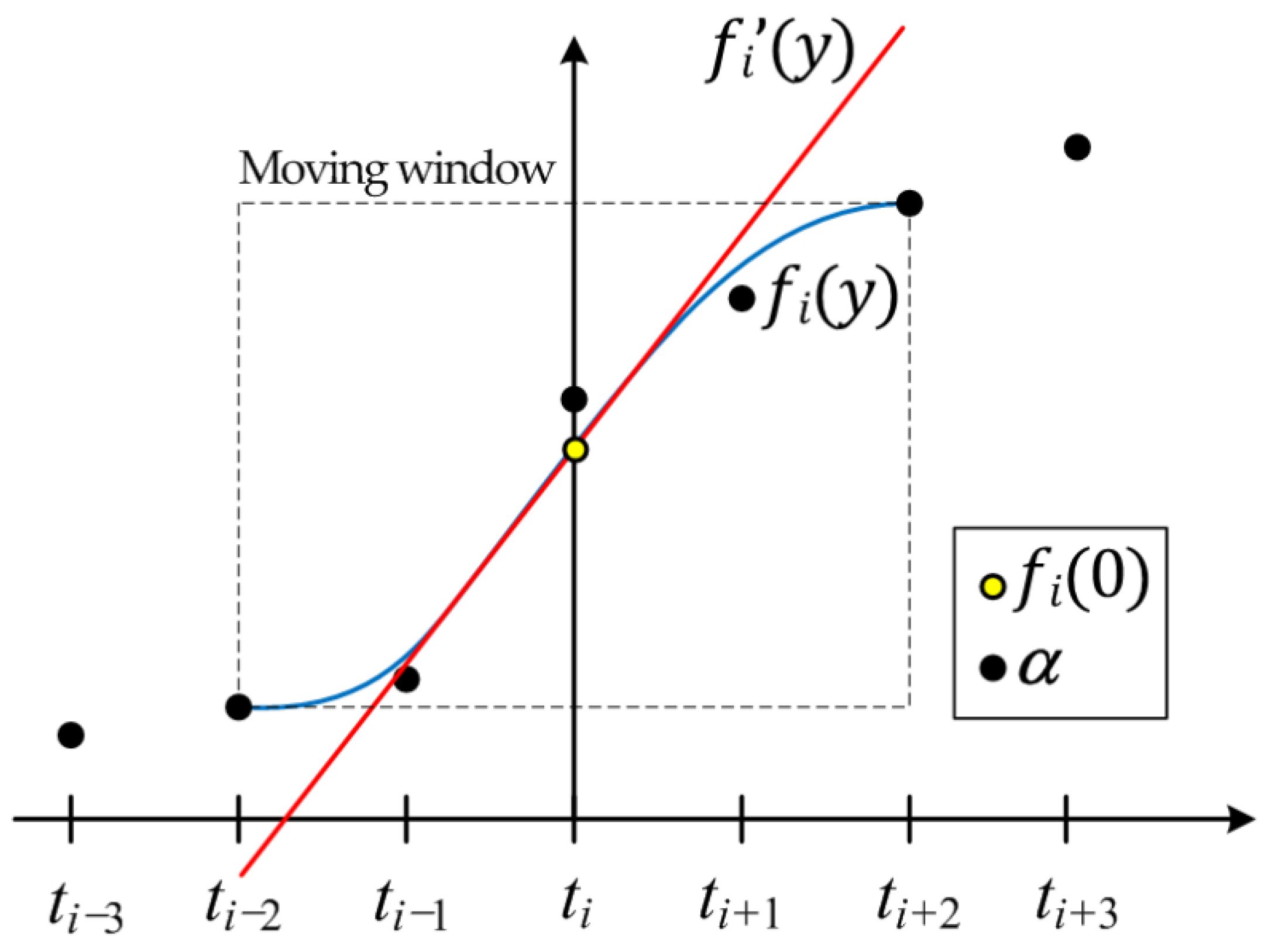
The aim of this paper was to build a practical method that can cope with the oscillations of S-curves due to the use of an oscillatory parent UH. It was assumed that the data of the hydrologic system are sampled at discrete times $t_i=iT$ for $i\ge 0$, where T is the sampling interval. For this system, the ordinates of the S-curve, $s\left(t\right)$, at $t_i=iT$ can be represented by the ordinate of $s_T\left[i\right]$. The SG filter approximates the S-curve as a piecewise continuous function $s_T\left(t\right)$ within a moving window around each data point $s_T\left[i\right]$. The ordinates of the S-curve are defined by ${\mathit{s}}_{\mathit{T}}={\left[s_T\left[1\right],s_T\left[2\right],\cdots ,s_T\left[N\right]\right]}^{{\rm T}}$, where N is the number of ordinates. The SG filter fits a polynomial to each subset of data points in the ordinary least-square (OLS) sense, and then it performs differentiation on the fitted polynomial.

Let each subset, including $2\mu +1$ S-curve ordinates, be placed symmetrically about the mid-point $\left(t_i,s_T\left[i\right]\right)$, where $2\mu +1$ defines the size of the moving window. The subset α is defined as:

$$\mathit{\alpha }={\left[s_T\left[i-\mu \right],\cdots ,s_T\left[i-1\right],s_T\left[i\right],s_T\left[i+1\right],\cdots ,s_T\left[i+\mu \right]\right]}^{{\rm T}}\in {\mathit{R}}^{2\mu +1}$$

(1)

Each subset of the S-curve is to be fitted by a polynomial of degree $\pi \left(\pi \le 2\mu \right)$. The r-th differentiation of the S-curve data at the mid-point is calculated by using the r-th derivative of the fitted polynomial. Note that the 0-th differentiation simply smooths the S-curve. The polynomial $f_i\left(y\right)$ of degree $\pi$ to be fitted through an ordinate $s_T\left[i\right]$ has the form:

$$f_i\left(y\right)={{\displaystyle \sum }}_{k=o}^{\pi }{b}_k{\left(\frac{t-t_i}{T}\right)}^k$$

(2)

where the polynomial $f_i\left(y\right)$ approximates $s_T\left(t\right)$, which is defined by ${\widehat{s}}_T\left(t\right)$; $y=\left(t-t_i\right)/T$; and, $b_i$ is the coefficient of the order-k term to be estimated:

$${\mathit{b}}^{\mathit{T}}=\left[\begin{array}{cccc}{b}_o& b_1& \cdots & b_{\pi }\end{array}\right]\in {\mathit{R}}^{\pi +1}.$$

(3)

For example, the relationship between $f_i\left(y\right)$ and $s_T\left[i\right]$ with respect to $t_i$ is illustrated in Figure 1 when $\mu =2$ (i.e., use of five S-curve ordinates).

Given the subset α, a basic matrix ${\mathit{G}}_{\left(2\mu +1\right)\times \left(\pi +1\right)}$ and its corresponding polynomial coefficient vector b can be expressed as follows [12,13]:

$$\mathit{G}=\left[\begin{array}{cccc}1& -\mu & \cdots & {\left(-\mu \right)}^{\pi }\\ ⋮& ⋮& ⋮& ⋮\\ 1& 0& \cdots & 0\\ ⋮& ⋮& ⋮& ⋮\\ 1& \mu & \cdots & {\left(\mu \right)}^{\pi }\end{array}\right]\in {\mathit{R}}^{2\mu +1,\pi +1}$$

(4)

$$\mathit{b}={\left({\mathit{G}}^{\mathit{T}}\mathit{G}\right)}^{-1}{\mathit{G}}^{\mathit{T}}\alpha =\mathit{Z}\mathit{\alpha }$$

(5)

where the matrix Z is the convolution coefficient matrix of the SG filter. Once the coefficient vector b is determined, the estimate of ordinate ${\widehat{s}}_T\left(t_i\right)$ can be obtained by ${\widehat{s}}_T\left(t_i\right)=f_i\left(0\right)$ for $t=t_i$ in Equation (2). Similarly, the r-th derivative of ${\widehat{s}}_T\left(t_i\right)$ can be written in the form:

$$\frac{d^r}{d{t}^r}{\widehat{s}}_T\left(t_i\right)=\left(\frac{1}{T^r}\right)\frac{d^r}{d{t}^r}f\left(0\right)$$

(6)

According to SG filter theory, Equation (6) can readily be re-written with matrix Z because each column of matrix Z contains the coefficients of each differentiation order. Consequently, the estimate of the r-th derivative of S-curve at time $t_i$ can be generalized in the matrix form as:

$$\frac{d^r}{d{t}^r}{\widehat{s}}_T\left(t_i\right)=\frac{r!}{T^r}{\mathit{e}}_{r+1}^{\mathit{T}}\mathit{Z}\mathit{\alpha }$$

(7)

where ${\mathit{e}}_r$ denotes the r-th unit vector. For example, for $r=1$, $e_2^{\mathit{T}}=\left[\begin{array}{ccccc}0& 1& 0& \cdots & 0\end{array}\right]\in {\mathit{R}}^{\pi +1}$. From these equations, the smoothed S-curve ${\widehat{s}}_T\left(t_i\right)$ is obtained as follows by substituting $r=0$.

$${\widehat{s}}_T\left(t_i\right)={\mathit{e}}_1^{\mathit{T}}\mathit{Z}\mathit{\alpha }$$

(8)

The IUH from the S-curve can be thus written in the form:

$$h\left(t\right)=\frac{d}{dt}s\left(t\right)=\frac{1}{i}\frac{d}{dt}{\widehat{s}}_T\left(t\right)$$

(9)

In another form using $\mathit{Z}$, we can obtain an estimate $\widehat{h}\left(t_i\right)$ of an IUH by substituting $r=1$ into Equation (7), which leads to:

$$\widehat{h}\left(t_i\right)=\frac{1}{i}\left(\frac{1!}{T^1}\right){\mathit{e}}_2^{\mathit{T}}\mathit{Z}\mathit{\alpha }={\mathit{e}}_2^{\mathit{T}}\mathit{Z}\mathit{\alpha }$$

(10)

2.2. Analysis and Discussion of Results

• Conventional method of deriving an S-Curve

A T-h S-curve is derived by adding a series parent T-h UHs that are lagged by period T. This S-curve represents the runoff hydrograph resulting from rainfall with an intensity of T⁻¹ cm h⁻¹. The S-curve asymptotically attains an equilibrium at the point when the inflow (excess rainfall) discharge and the outflow (runoff) are equal in amount. The equilibrium discharge $Q_{eq}$ (m³ s⁻¹) is determined by:

$$Q_{eq}=0.2778\frac{A}{T}$$

(11)

where A is the basin area (km²).

• Model performance evaluation criterion

The performance of conventional and SG filtered S-curve methods is evaluated by the Nash–Sutcliffe criterion [14] given in Equation (12).

$$E=\left(1-\frac{{{\displaystyle \sum }}_{j=1}^J{\left(q_j-{\widehat{q}}_j\right)}^2}{{{\displaystyle \sum }}_{j=1}^J{\left(q_j-\overline{q}\right)}^2}\right)\times 100$$

(12)

where E is the Nash–Sutcliffe model efficiency coefficient, J is the number of observations, $q_j$ is the observed runoff at time j, ${\widehat{q}}_j$ is the reproduced runoff at the same time j, and $\overline{q}$ is the mean of observed runoff. The value of E ranges from 0 to 100%. The closer E to 100%, the better the performance of the model. The peak relative error, QB, is the difference in magnitude between the observed and reproduced peaks and is used for acceptance analysis [15]:

$$QB=\frac{q_p-{\widehat{q}}_p}{q_p}$$

(13)

where $q_p$ is the peak value of observed runoff and ${\widehat{q}}_p$ is the peak of reproduced runoff. The closer QB to 0, the better the performance of the model.

3. Results

For single storm event data, the total number of direct runoff ordinates is generally small. Therefore, this study adopted the SG filter with minimum size $\left(\mu ,\pi \right)=\left(2, 2\right)$ to assess the applicability of the proposed methodology. The effect of the filter size is discussed in a subsequent section.

3.1. Derivation of Oscillation-Reduced UH

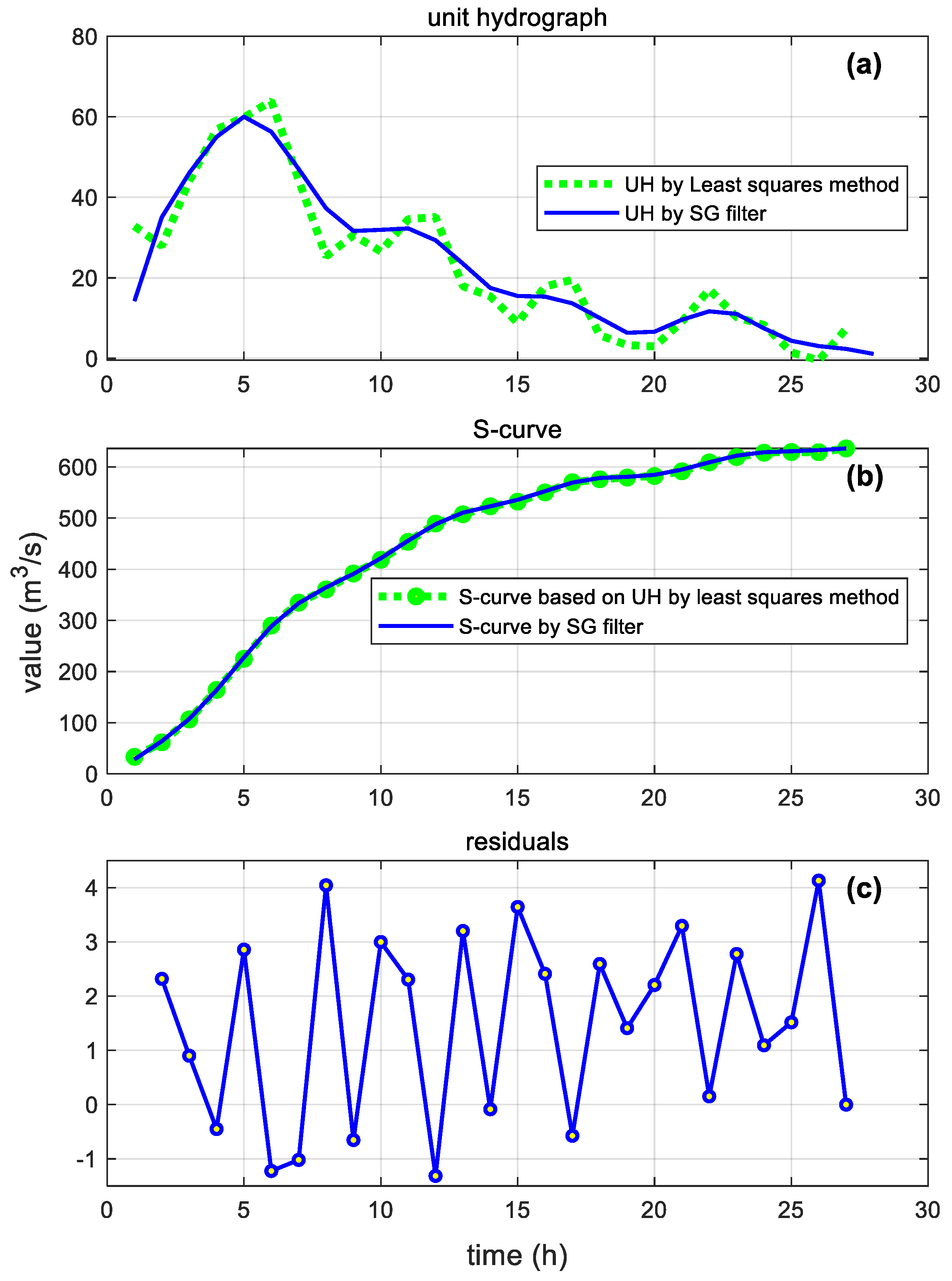
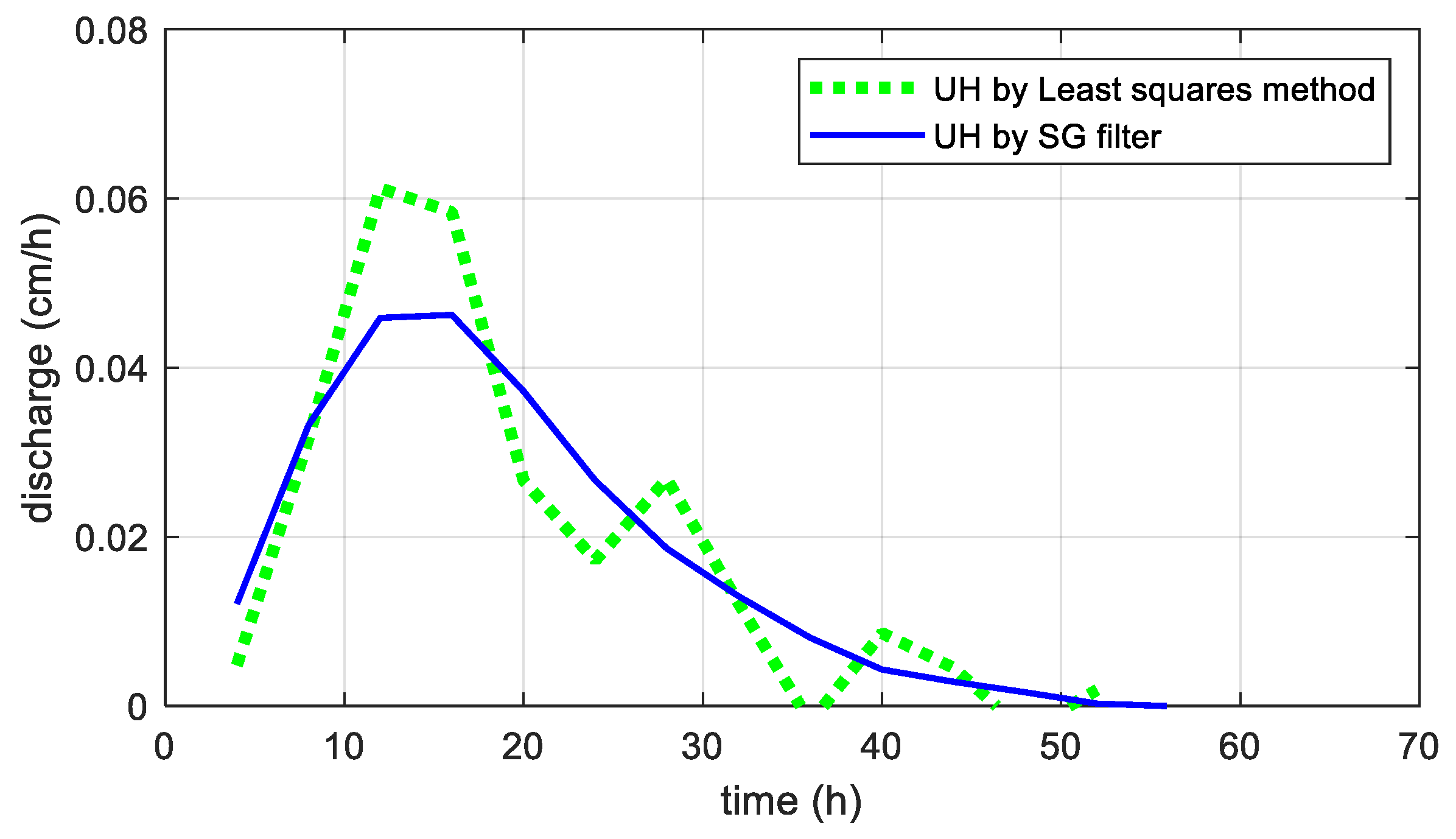
In this study, a reproduced T-h UH using an SG-filtered S-curve was compared to parent T-h UH obtained by OLS ($U{H}_{OLS}$). The considered storm event occurred in the Almond and Almondell basin (229 km²), Scotland, UK. The data were taken from [1] and were used to test the applicability of the ridge regression on regularization of UH oscillation in prior research.

The measurement interval T is one hour and the corresponding 1-h $U{H}_{OLS}$ could be calculated. Figure 2a plots this parent 1-h UH, in which strong oscillation can be observed all over the UH.

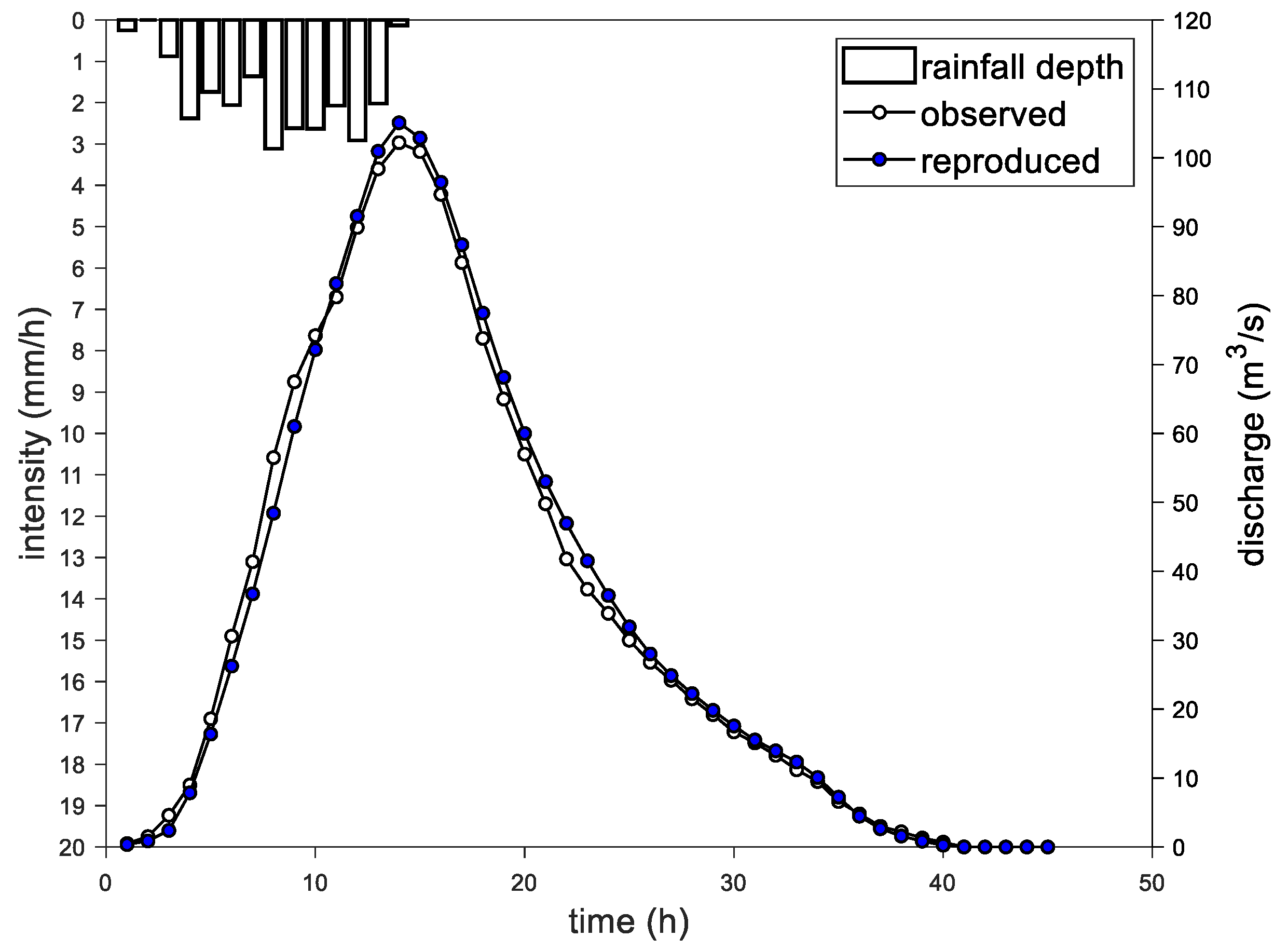
The 1-h conventional S-curve was developed by successively adding a series 1-h UHs lagged by duration T = 1 h until the base time (27 h) shown in Figure 2b. The equilibrium discharge $Q_{eq}$ was 636 m³ s⁻¹. The SG filter applied to this conventional S-curve with filter parameters $\left(\mu ,\pi \right)=\left(2, 2\right)$ readily gave a minimum influence on original data. In this process, a small adjustment to attain $Q_{eq}$ at the base time of the UH was necessary. The resulting SG filtered S-curve is compared to the traditional one in Figure 2b. In addition, the difference between the two S-curves is plotted in Figure 2c. The comparison of $U{H}_{SG}$ and $U{H}_{OLS}$ in Figure 2a indicates a significant reduction of oscillation. The UH parameters for $U{H}_{OLS}$ were determined to be $\left(t_p, q_p\right)=\left(6, 63.9\right)$, while $\left(t_p,q_p\right)=\left(5, 60.3\right)$, where $t_p$ = time-to-peak (h) and $q_p$ = peak flow rate (m³ s⁻¹), for $U{H}_{SG}$. The runoff hydrograph was reproduced by the obtained $U{H}_{SG}$ and effective rainfall, as shown in Figure 3, to evaluate the performance indices.

With E = 99.0%, the reproduced hydrograph was in good agreement with the observed hydrograph but slightly underestimated the peak. In addition, QB = 0.01, which indicated the excellent performance of the proposed method.

3.2. IUH Estimation Using SG Filter

It is widely accepted that differentiation is a roughening operator that magnifies errors in the calculation. Thus, the differentiation of S-curve using a general method (e.g., the finite difference method) is very likely to produce a more oscillatory IUH. Meanwhile, using the SG filter has the advantage of simultaneously smoothing and differentiating the S-curve.

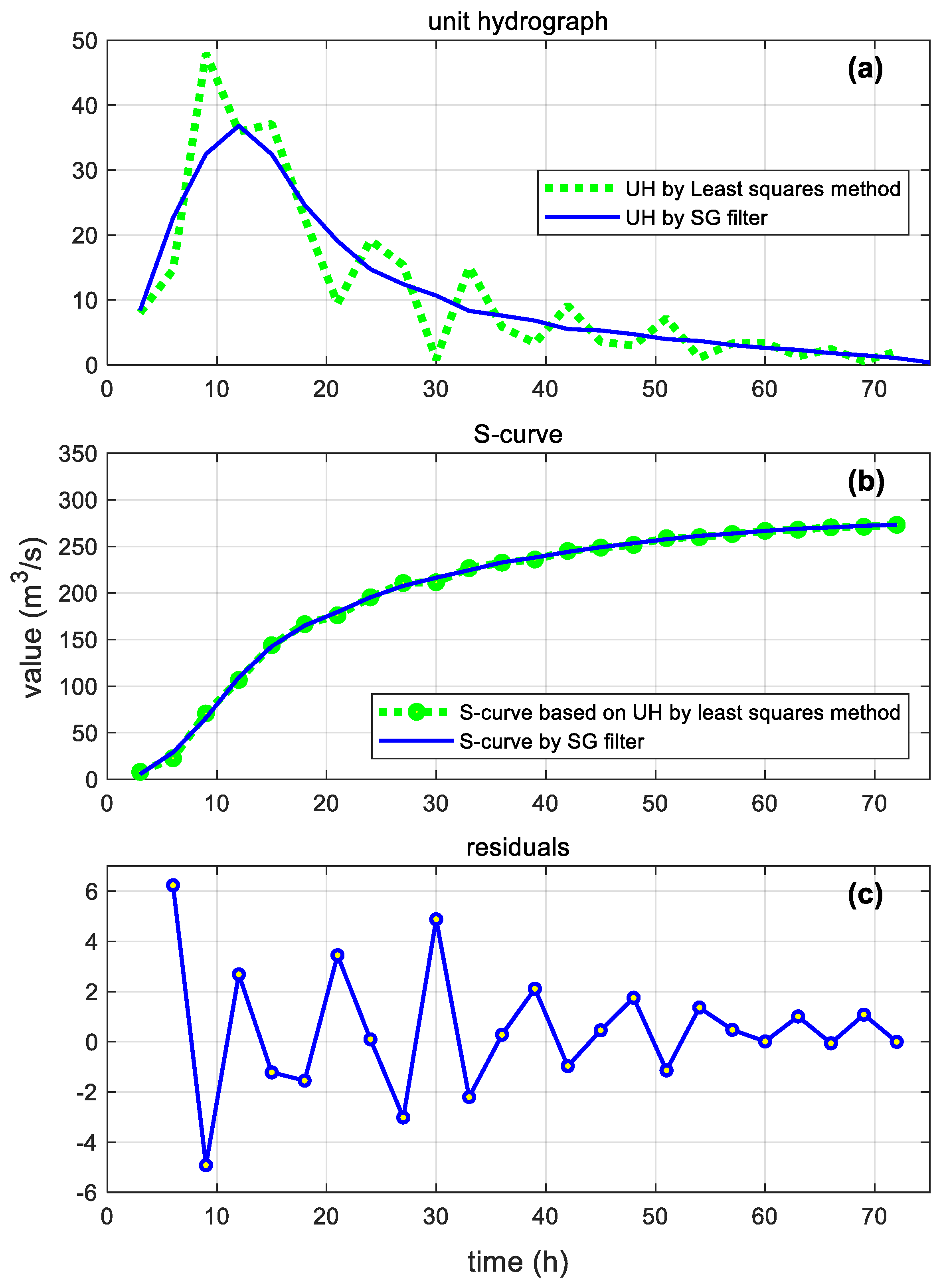
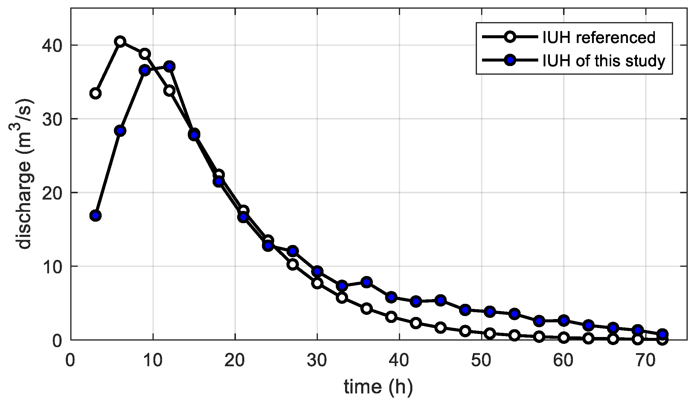
The considered storm event pertained to the Nenagh River basin (295 km²), Ireland. This event was carefully selected from 22 storm records and was identified by Event-14, in which the direct runoff hydrograph (DRH) was reported every 3 h with a peak discharge of 20.84 m³ s⁻¹. The corresponding depth of effective rainfall (ER) measured at intervals of 3 h during the event was 5.59 mm. Figure 4a plots a 3-h UH, in which a strong oscillatory UH was found when using OLS.

The 3-h conventional S-curve was developed by successively adding a series lagged by duration T = 3 h until the base time (72 h) shown in Figure 4b. The equilibrium discharge $Q_{eq}$ was 273 m³ s⁻¹. The S-curve was smoothed and differentiated using the SG filter with parameters $\left(\mu ,\pi \right)=\left(2, 2\right)$. The resulting SG filtered S-curve is compared to the S-curve obtained by a traditional method in Figure 4b. The residual between the above-mentioned two S-curves is shown in Figure 4c. It can be seen that the SG filter provided a remarkable improvement for oscillation. The resulting hydrograph $U{H}_{SG}$ based on the IUH is compared to $U{H}_{OLS}$ in Figure 4a. The UH parameters for $U{H}_{OLS}$ were determined to be $\left(t_p, q_p\right)=\left(9, 48.0\right)$, while those of $U{H}_{SG}$ $\left(t_p, q_p\right)=\left(12, 37.1\right)$.

The Nash IUH [16] could be represented as a basin IUH in the form of a gamma probability density function. The computed IUH was compared to the Nash IUH. For the same storm event, the reported parameter values were $\left(n,k\right)=\left(1.808, 2.705\right)$ [11], where n = number of linear reservoirs in series and k = reservoir storage coefficient. Figure 5 compares the obtained IUH to the Nash IUH.

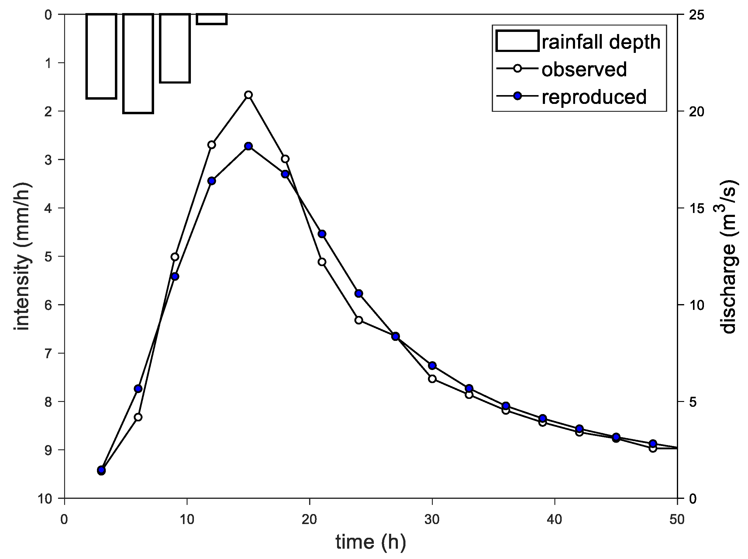
It can be seen in Figure 5 that it is likely that the IUH of this research was in practical accordance with the Nash IUH, despite the IUH of this study showing a lower and later peak. To evaluate performance indices, the runoff hydrograph was reproduced using convolution with $U{H}_{SG}$ obtained from the IUH and effective rainfall, as shown in Figure 6, to evaluate the performance indices.

The reproduced hydrograph was comparable to the observed hydrograph, with E = 97.9% but with a lower peak. QB was estimated to be 0.13, which indicated the fairly good performance of the proposed method. In view of these performance indices, the proposed method appeared to have been properly estimated the IUH.

3.3. Scale Problems for Using SG Filter

In theory, the Savitzky–Golay filter is most competent for much larger values of $\mu$ because the SG filter can accomplish only a relatively small amount of smoothing when using small values of $\mu$. Therefore, small watersheds with a short time-to-peak are likely to have a relatively poor applicability for SG filters unless the measurement interval time is short enough to increase the volume of data points. In addition, small and urbanized watersheds tend to have abrupt changes in values between the ordinates on S-curves during runoff time, since UHs of small and urbanized areas obtained by OLS frequently deviate the hydrological stability to a serious level. For this reason, one cannot expect any effect of the SG filter. Such a case is illustrated here.

The considered storm [17] pertains to the Shaol Creek watershed (11.25 km²), USA. The direct runoff hydrograph was reported at T = 0.5 h, with a peak discharge of 59.43 m³ s⁻¹. The corresponding depth of total rainfall measured at interval of 0.5 h during the event was 94.5 mm, and the value of the Φ-index was determined to be 23.6 mm h⁻¹ in this study. The S-curve was calculated and smoothed with filter parameters $\left(\mu ,\pi \right)=\left(2, 2\right)$. Figure 7 compares a reproduced S-curve to an S-curve developed by a traditional method that shows strong oscillations.

Based on the facts described above, the use of the SG filter only seems valid when the calculation time interval is narrow enough and there is no significant oscillation in the parent UH. This condition appears to be a hydrological problem concerning parent UH determination and not a problem with SG filter application.

It is accepted that the UH method should be used for basin areas smaller than 5000 km². Generally, wide watersheds have longer base times and provide sufficient runoff ordinates to the SG filter. Therefore, the analysis of a large basin was conducted in this study.

The data of rainfall runoff pertained to the North Potomac River near Cumberland, Maryland, USA (2266 km²). This event [18,19] was used to evaluate the applicability of the SG filtering method. The direct runoff hydrograph was measured at interval T = 4 h with a peak discharge of 0.356 cm h⁻¹. The corresponding depth of effective rainfall measured during the event was 7.12 cm. The 4-h $U{H}_{OLS}$ could be calculated. Figure 8 plots this parent 4-h UH, in which serious oscillation over the UH can be observed.

Here, the SG filter parameters were $\left(\mu ,\pi \right)=\left(2, 2\right)$. The resulting hydrograph $U{H}_{SG}$ is compared to $U{H}_{OLS}$ in Figure 8. The UH parameters for $U{H}_{OLS}$ were determined to be $\left(t_p, q_p\right)=\left(12, 0.061\right)$, while for $U{H}_{SG}$, $\left(t_p, q_p\right)=\left(12, 0.0495\right)$, where $t_p$ is in h and $q_p$ is in cm h⁻¹. The results of this basin showed no particular difference in UH shape from those of other watersheds. However, in Figure 8, the peak value is somewhat different, though the difference could be reduced by applying different values of SG parameters. The explanation for this is given in the next section.

4. Discussion

The oscillation of a UH is fundamentally generated by the combined effect of the intensity of the rainfall and the condition number of a covariance matrix in deconvolution formulation [10]. This covariance matrix is obtained from a rainfall matrix containing the volume of rainfall pulses. This means that the baseflow separation method affects the parameter values of the SG filter. Meanwhile, the baseflow separation method does not have a great impact on UH derivation when the baseflow is a small fraction of the flood hydrograph [15]. In this case, it can be assumed that the SG filter parameters are independent to baseflow separation. These facts indicate that the oscillation problem has not been completely resolved and emphasize the appropriateness of applying smoothing techniques [20].

The stability conditions accepted by hydrologists are that (1) a UH should not have negative ordinates, (2) a UH should be unimodal, and (3) a UH should be smooth. This study mainly considered smoothness when hydrological stability mainly depends on the error of the data. An important point about the UH obtained by OLS using error-prone data is that the shape of the UH may violate hydrological stability conditions. For this reason, the ridge least square (RLS) has been adopted to reduce the oscillation in a UH. However, the determination of ridge parameters has been subjective and difficult in hydrologic application [1]. In this study, SG filters were used for almost the same purpose as RLS. The advantage is that using the SG filter is less subjective and requires less computation than RLS. The most important role of SG filters is that the IUH can be estimated through the differentiation of the S-curve. The role of this SG filter is highly valuable because theoretical hydrology generally favors IUHs over UHs. Consequently, the use of SG filters is practically appropriate.

The idea of adopting SG filtering is to approximate or differentiate the specified S-curve within the moving window by a polynomial. It is known that SG filters are more useful for larger values of $\mu$ because filtering using small value of $\mu$ can only accomplish a relatively small amount of smoothing [21]. A quadratic or quartic order polynomial is typically used, and various combinations of parameters are possible. In this study, it was observed that the SG filter with the minimum filter size $\left(\mu ,\pi \right)=\left(2,2\right)$ was sufficient to give an acceptable performance. Similar results were obtained from the analyses of other storm events of the same watershed not reported in this research. The five-point weights of $\alpha$ used in Equations (8) and (10) for $\left(\mu ,\pi \right)=\left(2, 2\right)$ are given as fractional values in Equation (14):

$${\left({\mathit{e}}_1+{\mathit{e}}_2\right)}^T\mathit{Z}=\left[\begin{array}{ccccc}-3/35& 12/35& 17/35& 12/35& -3/35\\ -1/5& -1/10& 0& 1/10& 1/5\end{array}\right]$$

(14)

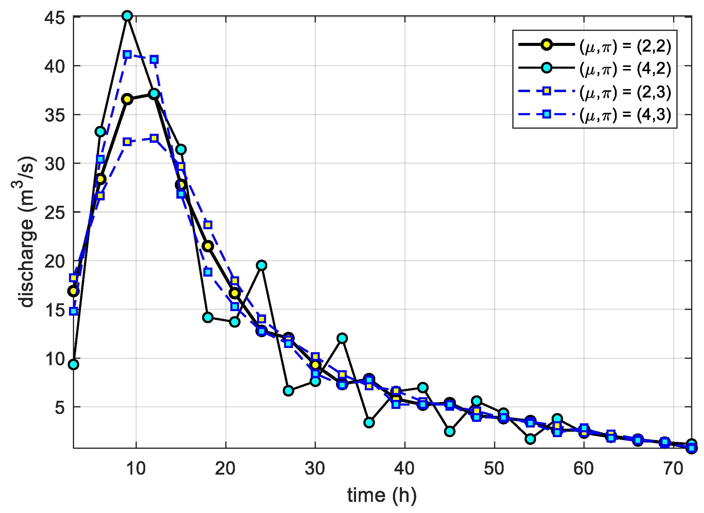
The SG filter can also employ different window sizes and polynomials of different orders to infer better values of weights. A plot comparing the IUHs for four different SG filter parameters with $\left(\mu ,\pi \right)$ = (2, 2), (2, 3), (4, 2), and (4, 3) is presented in Figure 9. It appears that lower values of $\mu$ rendered the UHs smoother but predicted a lower or later peak. In the case of $\pi$, there was no remarkable difference between $\pi =$ 2 and 3.

The performance indices of reproduced runoffs using four different parameter values are compared in

Table 1. Performance measure for selected Nenagh storm event with respect to four different parameter values of the SG filter.

Selected Parameter Values	Performance Indices
$\left(\mathit{\mu },\mathit{\pi }\right)$	E (%)	QB	NMSE
(2, 2)	97.948	0.127	1.269 × 10−9
(4, 2)	99.783	0.026	1.197 × 10−9
(2, 3)	95.037	0.203	3.094 × 10−9
(4, 3)	99.424	0.054	4.750 × 10−7

. To compare the acceptability of the SG filter model for each parameter set, the normalized mean square error (NMSE) was additionally considered. The NMSE emphasized scatter in dataset, and a smaller NMSE suggests better performance [15]. Like QB, the closer NMSE was to 0, the better the performance of the model. The values of the performance indices in Table 1 show that the SG filter performed well and showed a readily identical level of acceptability for the given range of parameters. Hence, each UH or IUH model using the SG filter can be accepted for forecasting runoff. However, since each model gives different UH or IUH shapes, it is necessary to select a well-smoothed one.

As mentioned in the considered case studies, the usefulness of SG filters depends on the window size. For the same storm event, the window size for filtering can be different depending on the computational interval. By the way, the setting of computational intervals is known to have a very important effect on peak and peak arrival time in hydrology [22]. Therefore, it is recommended that a minimum size filter be used for initial calculations in order to minimize the impact of filter, as well as that the filter parameters are adjusted to fit the observation runoff in subsequent calculations.

One important problem encountered in S-curve derivation is the oscillation near the equilibrium point. This study carefully investigated this behavior by varying the values of the SG parameters. The results revealed that the magnitude of the problem could be reduced, but the root cause remains a matter to be further investigated.

5. Conclusions

This study presented the application of digital filtering for developing and smoothing a non-parametric S-curve. For single storm event, deriving the S-curve is performed using the Savitzky–Golay filter (SG filter). The SG filter could be used to smooth S-curves and generate satisfactory IUHs from oscillatory parent UHs. The following conclusions can be drawn:

(1)

The SG filter provided a sufficiently applicable IUH. The proposed method was applied to the storm events of two basins with different areas, and the performance of the SG filter was evaluated through three different indices, the Nash–Sutcliffe model efficiency coefficient, the peak relative error, and the normalized mean square error, while considering four different parameter sets. All the considered SG filters were seen to perform similarly, with a slight advantage to the minimum size SG filter because it supported smooth enough S-curves and only required four numbers of adjacent ordinates in calculation.

(2)

Small watersheds with a short time-to-peak showed a relatively low applicability of SG filters because SG filter using a small number of data could only accomplish a relatively small amount of smoothing. However, this problem concerns the determination of the parent UH rather than SG filter application.

(3)

SG filters are effective methods for handling error-prone data, such as ridge-least square methods. Additionally, the SG filter has the advantage of less computational effort and being able to select objective parameters as compared to the ridge least squares. A quadratic polynomial based on five points of the SG filter appeared to be sufficient to reproduce runoff measured at an interval of one or three hour(s).

References

- Zhao, B.; Tung, Y.-K.; Yang, J.-C. Estimation of unit hydrograph by ridge least-squares method. J. Irrig. Drain. Eng. 1995, 121, 253–259. [Google Scholar] [CrossRef] [Green Version]
- Lattermann, A. System-Theoretical Modelling in Surface Water Hydrology; Springer: Berlin/Heidelberg, Germany, 1991. [Google Scholar]
- Ghorbani, M.A.; Singh, V.P.; Sivakumar, B.H.; Kashani, M.; Atre, A.A.; Asadi, H. Probability distribution functions for unit hydrographs with optimization using genetic algorithm. Appl. Water Sci. 2015. [Google Scholar] [CrossRef] [Green Version]
- Patil, P.R.; Mishra, S.K. Analytical approach for derivation of oscillation-free altered duration unit hydrographs. J. Hydrol. Eng. 2016, 21, 06016010. [Google Scholar] [CrossRef]
- Patil, P.R.; Mishra, S.K.; Jain, S.K.; Singh, P.K. An Analytical S-Curve Approach for SUH Derivation; Springer: Cham, Swizerland, 2021; pp. 349–360. [Google Scholar] [CrossRef]
- Yang, Z.; Han, D. Derivation of unit hydrograph using a transfer function approach. Water Resour. Res. 2006, 42, 1–9. [Google Scholar] [CrossRef] [Green Version]
- Subramanya, K. Engineering Hydrology, 4th ed.; McGraw-Hill: New Delhi, 2017. [Google Scholar]
- Ghosh, S.N. Flood Control and Drainage Engineering; CRC Press: Boca Raton, FL, USA, 2018. [Google Scholar]
- Savitzky, A.; Golay, M.J.E. Smoothing and differentiation of data by simplified least squares procedures. Anal. Chem. 1964, 36, 1627–1639. [Google Scholar] [CrossRef]
- Bree, T. The stability of parameter estimation in the general linear model. J. Hydrol. 1978, 37, 47–66. [Google Scholar] [CrossRef]
- Mohan, S.; Vijayalakshmi, D.P. Estimation of Nash’s IUH parameters using stochastic search algorithms. Hydrol. Process. 2008, 22, 3507–3522. [Google Scholar] [CrossRef]
- Orfanidis, S.J. Introduction to Signal Processing; Prentice Hall: Upper Saddle River, NJ, USA, 1996. [Google Scholar]
- Yoshimura, N.; Takayanagi, M. Chemometrics calculations with Microsoft Excel (5). J. Comput. Chem. Jpn. 2012, 11, 149–158. [Google Scholar] [CrossRef] [Green Version]
- Nash, J.E.; Sutcliffe, J.V. River flow forecasting through conceptual models part I—A discussion of principles. J. Hydrol. 1970, 10, 282–290. [Google Scholar] [CrossRef]
- Cleveland, T.G.; He, X.; Asquith, W.H.; Fang, X.; Thompson, D.B. Instantaneous unit hydrograph evaluation for rainfall-runoff modeling of small watersheds in North and South Central Texas. J. Irrig. Drain. Eng. 2006, 132, 479–485. [Google Scholar] [CrossRef]
- Nash, J.E. The form of the instantaneous unit hydrograph. Int. Assoc. Sci. Hydrol. 1957, 45, 114–121. [Google Scholar]
- Prasad, T.D.; Gupta, R.; Prakash, S. Determination of Optimal Loss Rate Parameters and Unit Hydrograph. J. Hydrol. Eng. 1999, 4, 83–87. [Google Scholar] [CrossRef]
- Bhattacharjya, R.K. Optimal design of unit hydrographs using probability distribution and genetic algorithms. Sadhana 2004, 29, 499–508. [Google Scholar] [CrossRef]
- Mays, L.W.; Coles, L. Optimization of unit hydrograph determination. J. Hydraul. Div. 1980, 106, 85–97. [Google Scholar] [CrossRef]
- Hunt, B. The meaning of oscillations in unit hydrograph S-curves. Hydrol. Sci. J. 1985, 30, 331–342. [Google Scholar] [CrossRef] [Green Version]
- Press, W.H.; Teukolsky, S.A.; Vetterling, W.T.; Flannery, B.P. Numerical Recipes in C; Cambridge University Press: Cambridge, UK, 1992. [Google Scholar]
- Kusumastuti, D.I.; Jokowinarno, D. Time step issue in unit hydrograph for improving runoff prediction in small catchments. J. Water Resour. Prot. 2012, 4, 686–693. [Google Scholar] [CrossRef] [Green Version]
Figure 1.
The scheme of the Savitzky–Golay smoothing differentiation filter using five ordinates of the S-curve.
Figure 2.
Hydrographs and S-curves by OLS and the SG filter (in the Almond and Almondell basin): (a) unit hydrographs before and after the application of the SG filter; (b) S-curves before and after the application of the SG filter; (c) difference between S-curve ordinates after the application of the SG filter.
Figure 3.
Comparison of observed hydrograph and hydrograph reproduced by the proposed procedure for selected storm (in the Almond and Almondell basin).
Figure 4.
Hydrographs and S-curves by OLS and the SG filter (in the Nenagh River basin): (a) unit hydrographs before and after the application of the SG filter; (b) S-curves before and after the application of the SG filter; (c) difference between S-curve ordinates after the application of SG filter.
Figure 5.
Comparison between IUHs derived by the Nash model and the proposed method for the selected storm.
Figure 6.
Comparison of observed hydrograph and hydrograph reproduced by the proposed procedure for selected storm (in Nenagh Basin).
Figure 7.
Comparison of S-curves before and after the application of the SG filter (in Shaol Creek watershed).
Figure 8.
Comparison of UHs before and after the application of the SG filter (in North Potomac River near Cumberland watershed).
Figure 9.
Effect on the instantaneous hydrographs due to variation of parameters of the Savitzky–Golay smoothing and differentiation filter.