Article

Hydrological Extremes and Responses to Climate Change in the Kelantan River Basin, Malaysia, Based on the CMIP6 HighResMIP Experiments

1
GeoInformatic Unit, Geography Section, School of Humanities, Universiti Sains Malaysia, Penang 11800, Malaysia
2
College of Engineering, Mathematics and Physical Sciences, University of Exeter, Exeter EX4 4QE, UK
3
Met Office, FitzRoy Road, Exeter Devon EX1 3PB, UK
4
Department of Meteorology, University of Reading, Berkshire RG6 6UR, UK
*
Author to whom correspondence should be addressed.
Water 2021, 13(11), 1472; https://doi.org/10.3390/w13111472
Submission received: 10 April 2021 / Revised: 6 May 2021 / Accepted: 20 May 2021 / Published: 24 May 2021

Abstract

:
This study introduces a hydro-climatic extremes assessment framework that combines the latest climate simulations from the Coupled Model Intercomparison Project Phase 6 (CMIP6) HighResMIP with the Soil and Water Assessment (SWAT) model, and examines the influence of the different climate model resolutions. Sixty-six hydrological and environmental flow indicators from the Indicators of Hydrologic Alteration (IHA) were computed to assess future extreme flows in the Kelantan River Basin (KRB), Malaysia, which is particularly vulnerable to flooding. Results show that the annual precipitation, streamflow, maximum and minimum temperatures are projected to increase by 6.9%, 9.9%, 0.8 °C and 0.9 °C, respectively, by the 2021–2050 period relative to the 1985–2014 baseline. Monthly precipitation and streamflow are projected to increase especially for the Southwest Monsoon (June–September) and the early phase of the Northeast Monsoon (December) periods. The magnitudes of the 1-, 3-, 7-, 30- and 90-day minima flows are projected to increase by 7.2% to 8.2% and the maxima flows by 10.4% to 28.4%, respectively. Lastly, changes in future hydro-climatic extremes are frequently quite different between the high-resolution and low-resolution models, e.g., the high-resolution models projected an increase of 11.8% in mean monthly flow in November-December-January compared to 3.2% for the low-resolution models.

1. Introduction

Climate change features pervasive global warming driven by anthropogenic emissions of greenhouse gases (GHGs), and is one of the major global threats that strongly affect the environment, ecosystems and human society. Intensification of precipitation and increases in temperature due to global warming have been observed in Asia in the past few decades [1,2,3]. These changes have a major impact on different hydrological systems and consequently increase the risk of regional water hazards such as flood and drought [4,5]. For example, damage caused by floods exceeds more than USD 10 billion a year in China [6,7]. Severe droughts can significantly reduce agricultural yields and freshwater supplies, resulting in social-economic losses [8]. Therefore, quantification of the climate change impact on precipitation extremes and subsequent extreme flows is important in developing better adaptation, more effective mitigation and greater resilience against water hazards.
The numerical modelling of the climate systems is one of the fundamental pillars in studying the changes in hydro-climatic extremes under different scenarios of anthropogenic GHG emissions. For such studies, general circulation models (GCMs) are extensively used to project scenarios of potential climate change across the earth system. Previous studies based on GCM experiments produced for the Coupled Model Intercomparison Project phase 5 (CMIP5) have projected a continuous global warming and increase in temperature extremes across the globe in the 21st century [9]. For hydrological research, outputs from the GCMs can provide useful driving data of hydrological models simulating the interaction between climate change and hydrological processes. Betts, et al. [10] applied the HadGEM3A-GA3.0, a high-resolution CMIP5 GCM (~60 km), to examine global freshwater availability under the RCP8.5 scenario. They noticed the water cycle changes are complicated and varied in different geographical regions, with mean river flow increase two times greater than the historical period in South and East Asia. A comparison of GCM resolution on a global hydrological cycle assessment was conducted by Vannière, et al. [11], who found increases in global precipitation from low to high resolutions models. However, uncertainties in the GCM simulations still require careful and more detailed consideration at basin scale.
A new generation of GCM simulations produced for Coupled Model Intercomparison Project Phase 6 (CMIP6) have been developed and released [12]. These experiments are based on state-of-the-art GCMs which are more capable of describing the complex physical processes within the climate system compared to the previous GCM versions [13]. The standard set of CMIP6 simulations are at relatively low resolutions of 100–200 km. However, the release of simulations from the High-Resolution Model Intercomparison Project (HighResMIP, Haarsma et al. [14]) for CMIP6 provides a good opportunity to study hydrological changes at unprecedented resolutions under present and future climates. Hence, application of the high resolution CMIP6 experiments in hydrological modelling at basin scale is likely to be a hotspot of hydrological research in the near future, especially for the impact assessment of hydrological extremes [15]. Previous studies based on regional climate models (RCMs) have found a considerable sensitivity of simulated basin-scale precipitation to changes in RCM model resolution, and such a resolution-dependance can have an impact on hydrological simulations [16,17]. However, considerable uncertainty remains both in RCM and GCM simulations requiring further investigation in order to understand how hydrological changes are influenced by the increase in model resolution. The availability of high-resolution GCMs from HighResMIP allows the comparison of different GCM resolutions and hydrological outputs, especially in the simulation of tropical extreme river flows, and provides a good opportunity to study the effect of model resolution on hydrological assessments. In particular HighResMIP provides simulations at resolutions similar to previous RCM based studies without the methodological uncertainties inherent in using RCMs, i.e., definition of the domain, nesting, nudging, etc.
In tropical Asia, extreme flows are sensitive to extreme climatic events, particularly in small catchments [18]. Numerous studies have investigated the impacts of climate change on extreme flows in different river basins over Southeast Asia [19,20,21], where the reported changes vary from place to place. Based on the recent Coordinated Regional Climate Downscaling Experiment—Southeast Asia (CORDEX-SEA) simulations, a drier climate condition is projected for the southern part of Southeast Asia by the end of the 21st century, while a wetter condition is mainly found in the northern region [22]. The recent study of Tan, et al. [23] introduced a SouthEast Asia HydrO-meteorological droughT (SEA-HOT) framework that integrates the RCMs simulations from CORDEX-SEA and SWAT for hydro-meteorological drought assessment in current and future climates. Although RCMs can provide useful high-resolution climate inputs for hydrological simulations, there are several known caveats. These include the lack of two-way interactions between the downscaled climate on the one-way nested grids and the external large-scale circulations [24,25]. The performance of RCMs is also strongly dependent on the selection of the driving lateral boundary conditions, e.g., Tangang, et al. [26], which can introduce considerable model uncertainties to climate simulations. Therefore, further studies are required to examine the hydrological simulations of SWAT driven by the latest high-resolution climate simulations, e.g., the CMIP6 HighResMIP experiments, which have a resolution similar to that of CORDEX-SEA.
To assess the hydrologic impacts on ecosystems, The Nature Conservancy (TNC) has developed the Indicators of Hydrologic Alteration (IHA) program, which is a software system that computes various hydrological and environmental indicators for quantifying the frequency, magnitude and duration of flows [27]. These indicators provide useful approaches to study flow behavior so as to improve the understanding of water hazards and their ecological and environmental impacts at a regional level. Several studies have combined the SWAT simulations with IHA to evaluate the impact of climate change on regional extreme flows [28,29,30]. Kiesel, et al. [31] integrated SWAT and 32 IHA indicators to evaluate future changes in extreme flows in three European catchments. Zhang et al. [32] used a similar approach to evaluate the impacts of cascade dams and climate variability on the streamflow of the Jiulong River watershed in the southeast of China. However, the simulation of SWAT combined with the analyses of IHA in tropical regions has been inadequately investigated in previous studies and requires further research, especially for Southeast Asia.
The Kelantan River Basin (KRB) is a typical tropical river basin in Peninsular Malaysia, which is frequently affected by monsoon floods during the early phase of the Northeast monsoon (NEM) season in almost every year [33]. In fact, previous major flood events in Malaysia were caused by continuous extreme precipitation episodes that were brought by the NEM associated with Madden–Julian oscillation (MJO) and the Borneo vortex [34,35]. According to Chan [36], one of the most destructive floods occurred in 1967, when more than 50% of the state’s population were affected. In 2014, the total amount of heavy precipitation from 21 to 23 December reached 1295 mm, and resulted in the highest water level of 22.7 m at the Jambatan Guillermard station [37], which is two times higher than the normal level. Tan et al. [38] evaluated the impact of climate change on water resources in the KRB based on the CMIP5 projections and found that the future annual streamflow will increase by 14.6 to 27.2%. This study also projected an increase in the monthly mean streamflow in November, December and January during the NEM season. However, these previous studies have provided limited information on the projected changes in extreme flows, which is critical for decision making in local water hazard risk management and environmental protection [39] across Kelantan. In addition, the SWAT calibration and validation of KRB have been mostly limited to monthly scale assessments. This study has further evaluated the capability of SWAT for a 30-year daily-scale simulation up to 2014.
Therefore, this study aims to introduce a framework to assess the impact of climate change on extreme flows in tropical regions through a novel approach that integrates SWAT, CMIP6 HighResMIP and the IHA indicators. The specific objectives are: (1) to evaluate the capability of CMIP6 HighResMIP at the basin scale; (2) to assess the SWAT capability in simulating long-term daily streamflow in the KRB; and (3) to quantify the hydrological extremes of the KRB in the mid-21st century period (1985–2014 vs 2021–2050) under high-resolution and low-resolution CMIP6 GCMs. The results of this study will enhance the understanding of how different HighResMIP CMIP6 GCMs resolutions influence the tropical extreme flow simulations. Besides, this study provides a comprehensive and the most up-to-date framework for assessing future hydro-climatic extremes for Southeast Asia as well as other tropical regions both in developing and less developed countries for climate adaptation and environmental protection policy formulations. Moreover, the future hydro-climatic projections can be used as a reference by the local authorities to design flood and drought related policies.

2. Materials and Methods
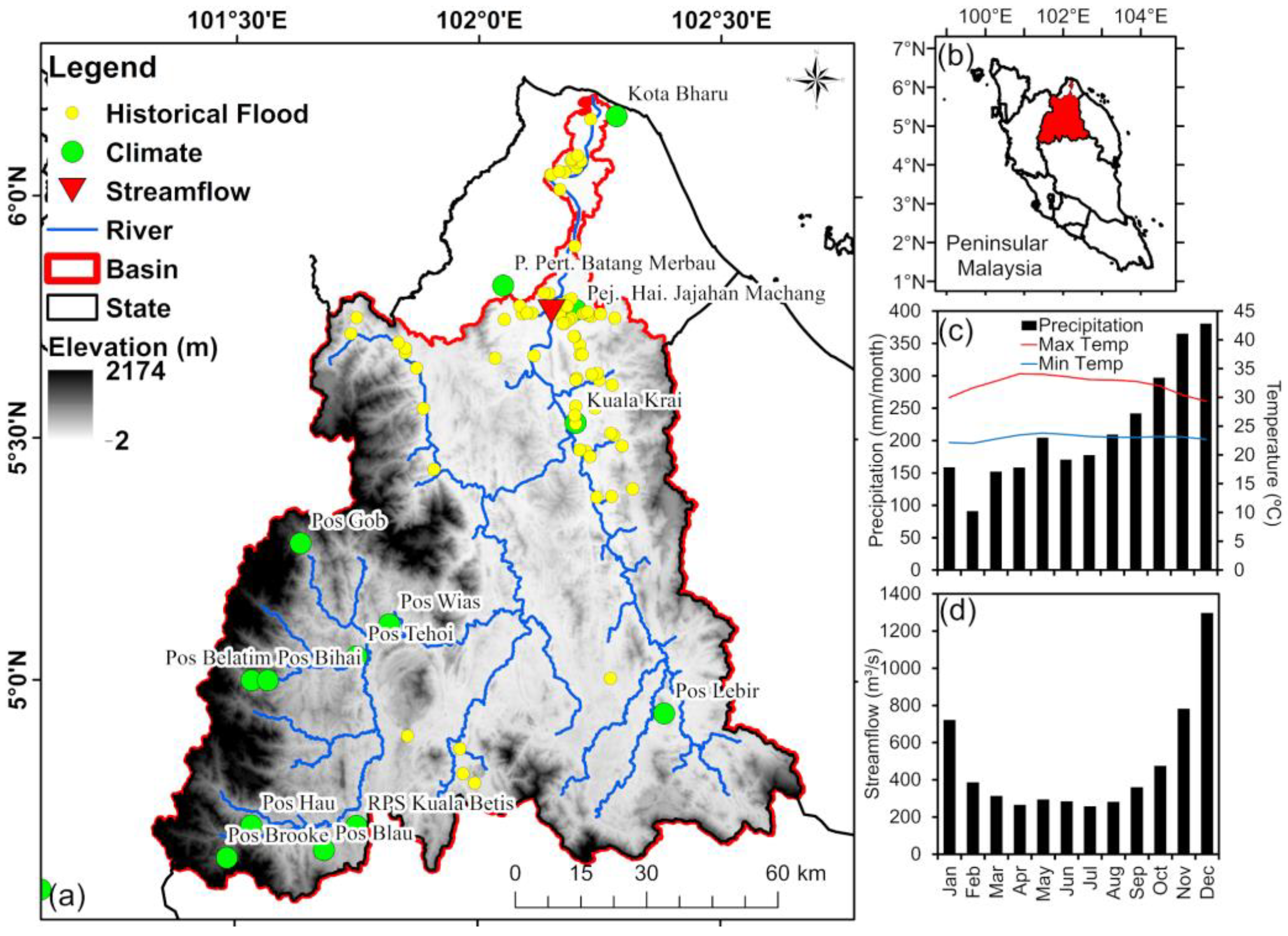
2.1. Study Area

The KRB is located in the northeast part of Peninsular Malaysia, between latitudes 4°–6° and longitudes 101°–103°, as shown in Figure 1. The Kelantan River originates from Mount Ulu Sepat. The elevation of the river basin ranges from −2 m to 2174 m. The river has a total length of 248 km and drains a basin area of 12,685 km2, covering more than 85% of Kelantan state. The outlet of this study was selected at the river mouth, so the drainage area is slightly larger than Tan et al. [38] who selected the Jambatan Guillermard streamflow station as the basin’s outlet. In 2013, the basin was dominated by forest (70.8%), followed by rubber (13.3%), oil palm (11.2%), agricultural (2.8%), paddy-fields (1.3%) and urban development (0.6%). Based on the flood reports prepared by the Department of Irrigation and Drainage Malaysia (DID), floods have normally occurred in Kuala Krai, Tanah Merah, Machang and Pasir Mas that are located in the middle and downstream parts of KRB. As reported in the DID’s 2014/2015 annual flood report, floods in Kelantan for the year 2014 resulted in the evacuation of more than 300,000 people, 14 casualties and about RM156 million total losses [40].
The KRB received an average annual precipitation of 2609.35 mm/year from 1985 to 2014, while average annual streamflow at the Jambatan Guillermard was 475.81 m3/s. Figure 1 shows the average monthly precipitation, maximum temperature, minimum temperature and streamflow for the basin from 1985 to 2014. The basin receives heavy precipitation during the early phase of the NEM season, mainly in November (365.4 mm/month) and December (380.74 mm/month). Relatively drier conditions can be found in the second phase of the NEM, where only about 91.3 mm/month precipitation is received in February. Average maximum and minimum temperatures of the basin vary from 29.3 °C to 34.1 °C and 22.0 °C to 23.8 °C, respectively. The highest temperature value is normally observed in April, the inter-monsoon period between the NEM and Southwest monsoon (SWM). The highest average monthly streamflow at Jambatan Guillermard is found in December (1296.3 m3/s), followed by November (781.9 m3/s) and January (721.3 m3/s), mainly during the flood periods in this region. As seen in Figure 1, precipitation is the dominant factor influencing the streamflow in the NEM, whereas temperature increases in the SWM raise evaporation and reduce flows. A moderate streamflow rate was found in the driest month of February, largely due to the lag of flows accumulated from the extreme high precipitation between November and January, where a similar situation was reported in other regions [41,42].

2.2. SWAT

The SWAT model is a semi-distributed and continuous hydrological model developed for water resources managers to decide the most appropriate strategy or solution by considering the impact of different management practices on streamflow and non-point source pollution [43]. SWAT has undergone continuous improvement over the past few decades [44,45] and its applicability and credibility have been verified in Southeast Asia [46]. SWAT is typically run at daily or monthly temporal resolution for a continuous period of time. The SWAT simulations can be driven by simulations of average flow climatology, while the representation of extreme flood events usually requires simulations driven at a finer (daily at least) temporal resolution. To simulate the long-term climatology of both extreme droughts and floods, a long-term climate simulation for at least 30-years at daily scale is recommended to be used as the SWAT input [15]. A review of SWAT-based hydro-climatic extremes studies has recently been reported by Tan [15]. About 47% of the studies were conducted in the United States and China. Besides that, only around 10% of the reviewed research has further evaluated both low and high flow conditions. Therefore, more studies in different geographical and climate conditions are needed to evaluate the capability of SWAT in capturing extreme flows.
The SWAT Calibration and Uncertainty Programs (SWAT-CUP), a tool designed specifically to calibrate and validate SWAT, is used in the SWAT model assessment [47,48]. The Sequential Uncertainty Fitting Version 2 (SUFI2) calibration program in the SWAT-CUP was selected to evaluate the model performance at daily and monthly scales. During the calibration, SWAT was run with 500 simulations per iteration under different parameter combinations. The Coefficient of determination (R2) and Nash-Sutcliffe Efficiency (NSE) [49] are the most commonly used statistical approaches to rate the performance of SWAT for each simulation. The R2 and NSE values range from 0 to 1 and −∞ to 1, respectively, with 1 being the optimal value for both metrics. Detailed descriptions and formulas of the two statistical approaches are available in previous SWAT studies [50]. Moriasi et al. [51] recommended that the performance of SWAT can be considered as satisfactory if NSE and R2 values are greater than 0.5 and 0.6, respectively.

2.3. CMIP6 HighResMIP Models

As an integral protocol of CMIP6, HighResMIP [14] provides high-resolution GCM ensemble simulations together with their coarse resolution versions. The HighResMIP experiments allow the assessment of the impact of model resolution on climate simulations and aim to improve the understanding of model biases and uncertainties [14]. This protocol acts as an important input to the Intergovernmental Panel on Climate Change (IPCC) sixth assessment report (AR6). The high resolution (<50-km) GCM simulations from HighResMIP also help to solve the issue of coarse model resolution in the CMIP5 GCMs [52] and are comparable to resolutions used in many RCM based studies [53,54]. In this paper, ten HighResMIP experiments for the present-day (1980–2014) and future (2015–2050) climates are chosen and the data are collected via the data platform of the Earth System Grid Federation. The future period simulations are based on the high-emission 8.5 scenario of the Shared Socioeconomic Pathways (SSPs-8.5), which is part of the new scenario framework for the latest IPCC climate change assessment. Descriptions of these models including the model developers and horizontal model resolutions are given in Table 1.
High resolution models have been demonstrated to offer greater fidelity than coarse resolution models in representing both the observed mean and extreme precipitation events over Peninsula Malaysia [55]. Nevertheless, even the high resolution models of HighResMIP inevitably show biases in their representation of extreme precipitation. Prior to applying the selected HighResMIP experiments to the simulation of SWAT and the subsequent assessment of hydrological impacts, the model biases relative to climate observations in the simulated climatic variables (i.e., daily precipitation, maximum and minimum temperatures) are corrected using a quantile mapping (QM) approach similar to Boé et al. [56] and Kim et al. [57]. QM first calculates the correction parameter (defined as the observed mean value divided by the simulated value) at different quantile levels. Corrected variables are then obtained by the product of the simulated value and the calculated correction parameter for each quantile level with an interval of 0.5 percentile rank. To correct the model bias in simulating the annual cycle of climatic variables, QM is applied to data for each month, respectively. To compare the simulations between low and high resolutions, the ensemble of the low resolution (LR) simulations from HadGEM3-LM, CNRM and FGOALS-L is analyzed and compared to the ensemble of the high resolution (Ens_HR) simulations from the other seven models.

2.4. IHA Indicators

IHA is a user-friendly tool developed by The Nature Conservancy to measure flow characteristics using 32 IHA (Table 2) and 34 Environmental Flow Component (EFC) (Table 3) indicators [27]. For example, the IHA tool can calculate the magnitude and duration of annual minima and maxima flows for specific periods, e.g., 1-day, 3-day, 7-day, 30-day, 90-day. These indicators provide useful information for policy makers, water managers, hydrologists and researchers to understand the impact of human activity, including land use and anthropogenic climate warming, on rivers and groundwater. Comparative analysis can be conducted to describe and quantify the changes of these extreme elements associated with climate change. The zero-flow day indicator is excluded in this study due to its limited suitability for tropical regions. The IHA version 7.1 is used to calculate the extreme flows based on the SWAT outputs. The computation of IHA is based on the daily streamflow data generated from the SWAT simulations.

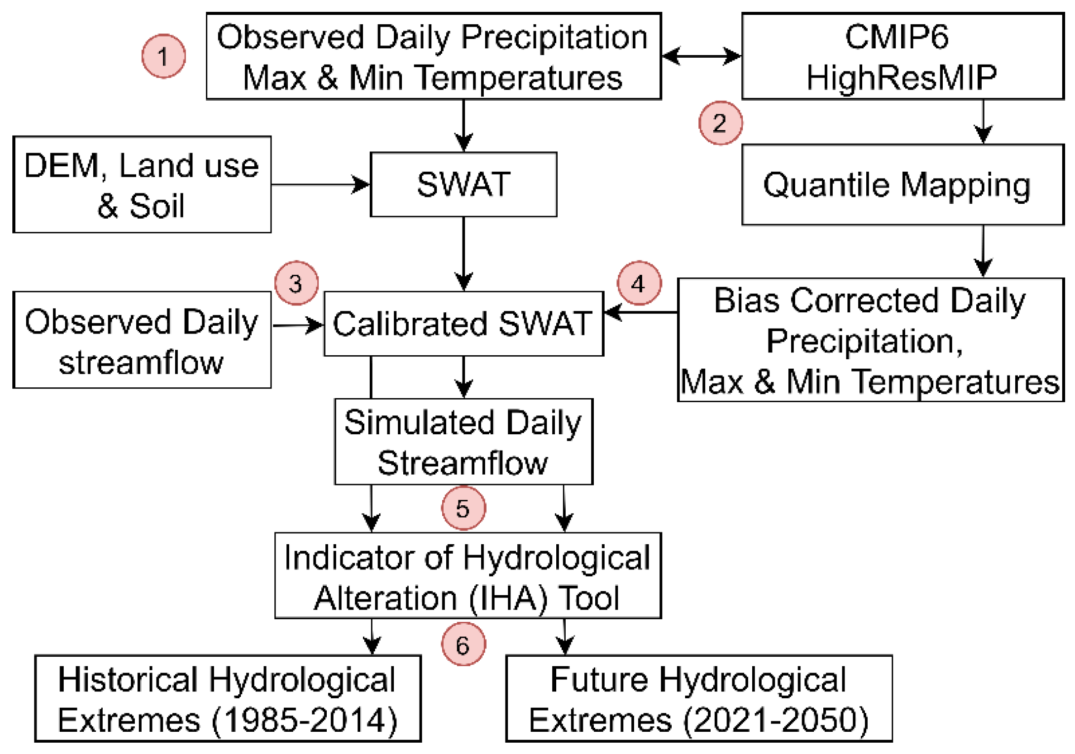
2.5. Model Setup and Input Data

The general framework of this study is shown in Figure 2 and includes the following steps: (1) SWAT input collection, (2) HighResMIP data download and bias correction; (3) SWAT calibration and validation; (4) Incorporation of the bias corrected HighResMIP into calibrated SWAT, (5) calculation of flow extremes based on the IHA indicators, and (6) comparison of the changes between future (2021–2050) and historical (1985–2014) flow extreme.
The simulation of SWAT requires three geophysical inputs, including land use, soil and elevation. The latter information was extracted from satellite-based digital elevation model data, the Shuttle Radar Topography Mission (SRTM). The land use data of 2013 is provided by the Department of Agricultural Malaysia (DOA), while the soil data is from the FAO-UNESCO soil map. The climate driving data of SWAT includes daily precipitation, daily maximum and minimum temperatures. Daily climate data from 1980 to 2014 was collected from the Malaysia Meteorological Department (MMD). To initialize the sub-basin delineation, digital river network data collected from Department of Drainage and Irrigation (DID) was used to integrate into the SRTM DEM for improving the river network formation. Lastly, the streamflow data from the same department is used to calibrate and validate the SWAT model. The minimum threshold value of 10,000 ha was used in the sub-basin delineations. Five slope classes of 0%–10%, 10%–20%, 20%–30%, 30%–40% and >40% were used in the slope definition during the model development. The next step is the formation of hydrologic response units, the smallest spatial unit of SWAT which lumps together all similar land uses, soils and slopes within each sub-basin to perform all model calculations.
SWAT has exhibited a reliable performance in simulating the climatology of monthly streamflow in Kelantan and typical cases of historical drought events [23,38]. This will apply a new configuration of SWAT, calibrated by referring to parameter ranges and sensitivity analysis from previous studies [23,38]. The calibration and validation periods are chosen as 1985–1999 and 2000–2014, respectively. As the SWAT model setup at the monthly scale has been well configured and described in previous studies [23,38], this paper focuses on the daily scale simulation, which is important for allowing the diagnoses of extreme flows.
Bias corrected HighResMIP climate projections as described in Section 2.3 are used to drive the calibrated SWAT in order to simulate the future daily streamflow from 1985 to 2050. Thus, the projected hydro-climatic changes driving the simulation of SWAT are based on multi-GCM ensemble experiments, which help to consider the climate projection uncertainties associated with the different GCM configurations and improve reliability in the assessment of hydro-climatic impacts [58,59]. The simulated streamflow will then be used to calculate the 66 extreme indicators as listed in Table 2 and Table 3. The assessment of climate change impact on flow extremes was conducted by comparing the relative differences of extreme indicators between 1985–2014 and 2021–2050. Moreover, the statistical significance of the mean difference between the future and the baseline historical periods at a 95% confidence level (p-value < 0.05) will be determined using the two-tailed Student’s t-test.

3. Results

3.1. SWAT Calibration and Validation

Table 4 indicates that the baseflow alpha-factor (ALPHA_BF), initial SCS runoff Curve Number for moisture condition II value (CN2) and effective hydraulic conductivity in main channel alluvium (CH_K2) are among the most sensitive parameters for daily streamflow calibration, which is similar to the previous monthly scale calibration in KRB [23,38]. ALPHA_BF shows the baseflow response to changes in recharge, CN2 represents a function of the soil permeability, land use and soil water condition, while CH_K2 adjusts the relationship of water exchange from groundwater to river [60,61].
The comparison between the observed and simulated streamflow in the case of Jambatan Guillermard during the calibration (1985–1999) and validation (2000–2014) periods is shown in Figure 3. In general, the simulated monthly and daily variations of streamflow are captured reasonably well with respect to the observed streamflow. However, an overestimation of baseflow is found for the period of 2010–2014, which is possibly due to increasing groundwater demand in recent years [62], as there is no accessible groundwater extraction data for the study area. Six groundwater parameters were considered in the SWAT calibration by allowing more water transfer from baseflow to surface or atmosphere so that the impact of inadequate groundwater data is minimized.
The model performance is rated as “very good” in terms of the monthly scale simulation according to the Jambatan Guillemard Bridge for both the calibration (R2 = 0.84 and NSE = 0.72) and validation (R2 = 0.84 and NSE = 0.63) periods. The performance of SWAT is rated as satisfactory at the daily scale. For the last iteration of calibration, 78% (p-value = 0.78) of the simulations were bracketed by the 95 Percent Prediction Uncertainty (95PPU) with r-value of 0.89, indicating that the calibration is acceptable. Thus, the calibrated configuration of SWAT will then be used for simulating the hydro-climatic extremes in the KRB and the results will be discussed in Section 3.3, Section 3.4 and Section 3.5.

3.2. Bias Correction of CMIP6 HighResMIP Models

The biases of the HighResMIP experiments were corrected using the QM, as discussed in Section 2.3. Figure 4 shows the climatology of monthly precipitation and maximum and minimum temperatures from 1980 to 2014 over KRB that are measured from observed data, original and bias-corrected HighResMIP models. The original HighResMIP models tend to underestimate the monthly precipitation in November and December, whereas an inconsistent pattern was found for other months. The HighResMIP models simulate the peak monthly precipitation in November, one month earlier than observed. The FGOALS-f3-L simulation exhibits a generally poorer performance than the other simulations as it significantly underestimates the precipitation amount over KRB, especially during the SWM season (June–September). We also note that the original HighResMIP models generally show a better performance in simulating the precipitation amount compared to the original regional climate model simulations from CORDEX-SEA that dramatically overestimate the observed precipitation by up to five times for certain months in the same basin [23]. As shown in Figure 4d, the QM approach reasonably corrects the biases of the models in representing the peak monthly precipitation in December and precipitation amount for all the simulations. It is also noted that the high resolution (HR) simulations exhibit less underestimation of precipitation during the NEM compared to low resolution (LR).
In general, most CMIP6 HighResMIP models reasonably capture the observed warm period in April and September in terms of the monthly mean of daily maximum and minimum temperatures (Figure 4b,c,e,f), mainly during the inter-monsoon periods. However, all the HighResMIP models underestimate the monthly maximum temperature, whereas most of the models show an overestimation in the monthly minimum temperature, except the CNRM-CM6-1-HR, EC-EARTH3P and GFDL-CM4C192 models. Minimum temperatures outperformed maximum temperatures in the climatology simulations since the ensemble mean is much closer to the observed data. Similar to precipitation, maximum and minimum temperature biases reduce significantly after applying the QM bias correction approach, as shown in Figure 4e,f, respectively. Compared to LR, the HR simulations show less overestimation of daily minimum temperature. However, no apparent improvement in simulating maximum temperature is found in HR.

3.3. Climate Change

The projected annual and monthly changes in precipitation, daily maximum and minimum temperatures over the KRB for the period 2021–2050 relative to 1985–2014 are shown in Figure 5. Annual precipitation is projected to increase significantly by 6.9%. For almost every month, the precipitation amount is projected to increase from 0.94 (October) to 15.1% (December), except for April with a reduction of 2.4%. In Figure 5a, statistically significant changes in the monthly average precipitation are seen in June, July, August and December, indicating a general increase in precipitation during the SWM and the early phase of the NEM.
The annual mean of daily maximum and minimum temperatures for the period 2021–2050 relative to 1985–2014 are projected to increase by 0.8 and 0.9 °C, respectively (Figure 5b). The equivalent warming trends are slightly higher than the historical long-term warming trends (0.1 and 0.3 °C/decade for maximum and minimum temperatures respectively) from 1985 to 2018 in Malaysia [1]. For each month, maximum and minimum temperatures are projected to increase by 0.7–1.0 °C, with higher magnitudes of warming in May and November (Figure 5b). There is also a significant difference between the future and historical temperatures in their mean values for both the annual and monthly scales (Figure 5b), supporting the literature regarding a warming situation in the next 30 years.

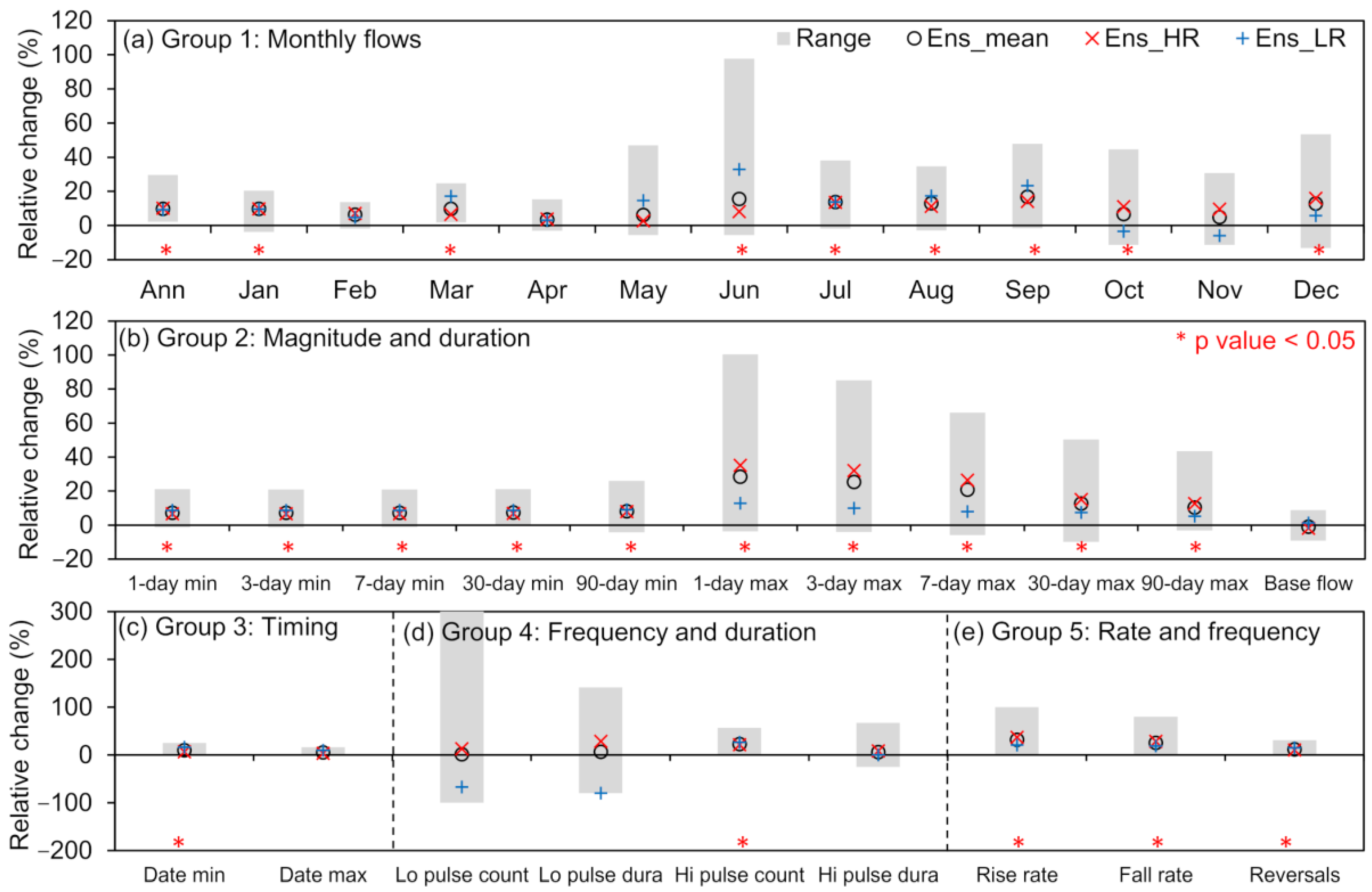
3.4. Hydrologic Extreme Changes

A comparison of the changes in hydrological extremes at the Jambatan Guillemard station between the 2021–2050 and 1985–2014 periods is shown in Figure 6. Annual and monthly streamflow are projected to increase by 9.9% and 3.5% to 16.8% in the future, respectively, as simulated from an ensemble mean of the ten HighResMIP models. A higher rate of increase of more than 10% can be found in June to August and December. Additionally, a significant difference of mean streamflow at 95% confidence level can be found at the time-scales of annual, December to January, March, and June to October, which is similar to the monthly precipitation changes. As December and January are the major flood periods in the KRB, more intense flooding impacts may occur in the future.
Next we analyze the indicators quantifying the annual streamflow extremes in terms of their magnitude for different durations, e.g., the second IHA group listed in Table 1. Figure 6b shows that the 1-, 3-, 7-, 30- and 90-day minima and maxima flows increase significantly from 7.2% to 8.2% and 10.4% to 28.4%, respectively, in the 2021–2050 period. There is a high deviation for the case of extremely high flows at 1-, 3- and 7- day maxima flow, showing that the magnitude of floods might increase in the near future. As for the baseflow index, a slight decrease of 0.9% is seen for the future period. This indicates that the future amount of water available for freshwater supply tends to remain the same as the current value. However, stress on water supply may occur if there is an increased water demand following population growth in the future.
The third IHA group indicates the streamflow extreme events in terms of the occurrence timing. A water year is defined using the Julian dates format where “day 1” refers to 1st January and “day 365” refers to 31st December. As shown in Figure 6c, the occurrence timing of the future annual minimum and maximum events that are projected by the ten models will increase by 1.0% to 25.3% (1.87 to 46.27) and 0.4% to 16.2% (0.73 to 29.67), respectively. This indicates that the future streamflow extreme events are projected to be delayed for a few days to a few weeks. The fourth IHA group shows the number and duration of extreme pulses. The results show that the number of low pulses showed no significant changes; meanwhile, the number of high pulses is projected to increase significantly by 22.7%. The duration of future low and high pulses tends to change slightly compared to the historical period, based on an ensemble mean of 3.3% and 5.9%, respectively. The last IHA group contains the rate and frequency of water condition changes. There is a significant increase in the rise rate and fall rate at the Jambatan Guillermard station by 31.9% and 25.5%, respectively, showing that a rapid increase or decrease in streamflow might happen in the future. The number of hydrological reversals will increase by 11.6% as projected by the model ensemble, which shows an increment in the number of daily streamflow increases after decreasing, and decreases after increasing.

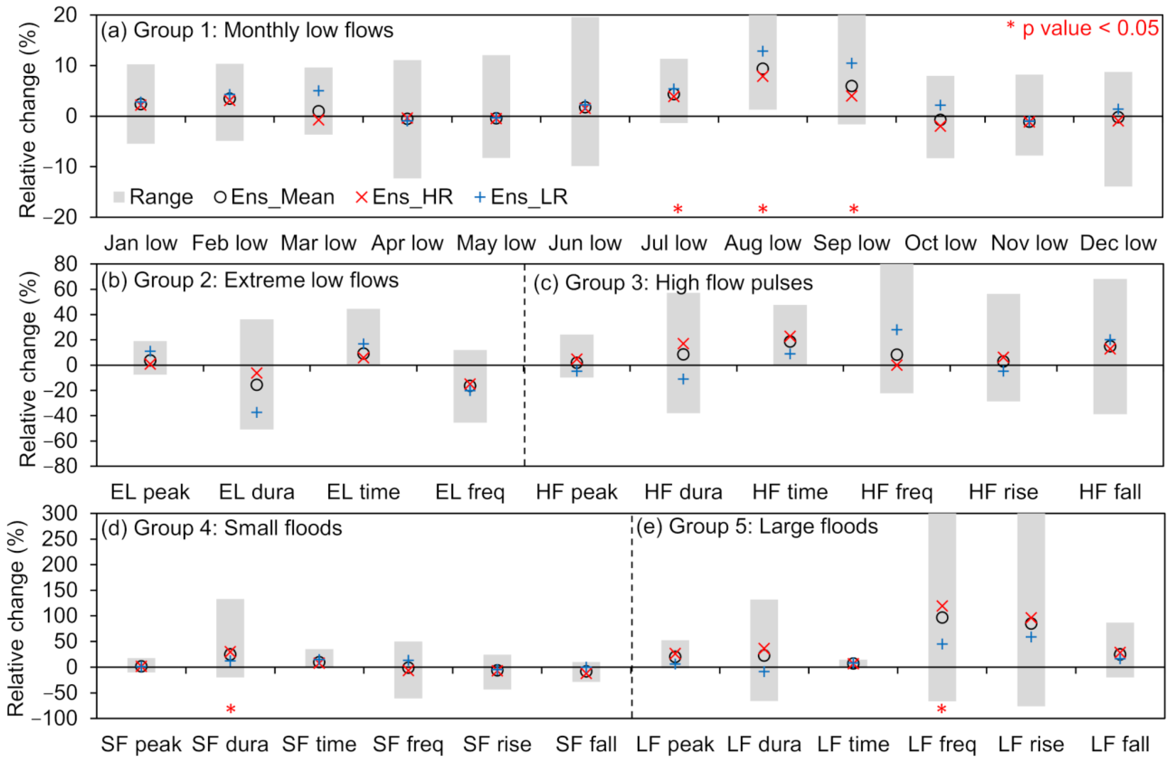
3.5. Environmental Flow Changes

The EFC indicators that divide into monthly low flows, extreme low flows, high flow pulses, small floods and large floods, were also considered in this study because this information is very important to sustain riverine ecological integrity. The first EFC group shows the monthly low flow sustained by groundwater, so any changes in these parameters can be related to groundwater availability. Basically, a slight decrease in the monthly low flow can be found in April, May and October to December by 0.2% to 1.1%, based on the ensemble mean projection as shown in Figure 7. By contrast, monthly low flows from July to September are projected to increase significantly at the 95% confidence level by 4.3 to 9.4%.

4. Discussion

Climate change is expected to have a more significant impact on hydrological extreme flows than environmental flow components, since more IHA indicators (Figure 6) were found to be significant in the 2021–2050 period than EFC indicators (Figure 7). The findings show that extreme high flows are more sensitive to climate than normal and low flows in the KRB. The situation can be highlighted by the fact of continuous heavy precipitation in the first week of January 2021, that resulted in serious flooding in five states of Peninsular Malaysia, including Kelantan. According to the Kelantan e-flood portal, https://ebanjir.kelantan.gov.my/ (accessed on 20 March 2021), water levels at the Jambatan Guillermard station exceeded the danger level of 16 m from 6th January to 9th January 2021, up to the peak level of 18.89 m. The water level is only slightly lower than the Kelantan Big Yellow Flood of 2014 that reached a peak level of 22.74 m. The alteration in extreme flows has a great influence on biodiversity and the ecological system within and surrounding the river [63].
The statistical analysis has shown that the SWAT model is acceptable for daily streamflow simulations in the KRB. In Southeast Asia, a review of SWAT application in hydro-climatic extreme studies reported that the SWAT model tended to have a better performance on monthly time scales compared to daily time scales [46]. A possible explanation for this might be insufficient rain gauges in the tropics to capture the daily-scale extreme precipitation at a better spatial coverage [64]. For example, the only rain gauge in the southeastern part of the KRB as shown in Figure 1 may miss captured extreme events in the nearby region, and therefore the extreme flows were underestimated by the SWAT model. In fact, the reported NSE and R2 values at daily time scales in previous SWAT extreme related studies commonly ranged from 0.50 to 0.79 [15]. Besides, the SWAT model tends to underestimate the peak flows which are reported in the river basins of Spain [65], Brazil [66] and Hawaii [67]. Based on Krysanova and Arnold [68], the flood-plain deposition algorithm within SWAT needs to be improved in order to increase the accuracy of SWAT in replicating peak flows. This suggestion has been taken into consideration during the SWAT+ development [69]; however, how effective the improvement is still needs further investigation.
Climate projections are always regarded as one of the major uncertainties in hydro-climatic impact modelling [15,70]. Given that the HR models have been shown to have a better fidelity in representing precipitation extreme events when compared to observations than their LR model counterparts [55], one might expect the HR models to provide a more accurate assessment of future precipitation extremes. Of the models assessed in this study, changes in future precipitation extremes are frequently quite different between the HR and LR models. The mean precipitation change is significantly higher during the November-December-January period when most flooding occurs at 9.6% for the HR models compared to 5.0% for the LR models (Figure 5). The associated mean monthly flow changes are significantly higher during the Nov-Dec-Jan period at 11.8% for the HR models compared to 3.2% for the LR models. The changes in the magnitude and duration of the 1-day to 90-day maximum flows are universally greater in the HR models than in the LR models with values for 1-day maxima increases by as much as 35.1% for HR compared to 12.8% for LR models (Figure 6). Large flood event marker changes in future climate scenarios are significantly more prevalent in the HR models than the LR models. For example, the large flood frequency increases by 119% for the HR models compared to 44.4% for the LR models (Figure 7). Similarly, Troin [71] also reported that RCM is superior than GCMs for hydro-climatic assessment, particularly in mountainous regions. Therefore, numerous high-resolution GCMs along with different downscaling techniques should be considered in future hydro-climatic modelling [72].
This intercomparison of simulations at different model resolutions suggests that the simulation results based on climate simulations at relatively low model resolutions should be interpreted with cautions. The linkage between the model performance in simulating regional precipitation and the spatial resolution of the model is complex. For example, Liang et al. [55] found that the high resolution version of HadGEM3-GC3.1 has a stronger ability to simulate the Borneo Vortices during the NEM season and their associated precipitation in Malaysia compared to the low resolution versions. This partly explains that the high-resolution simulations of MRI-S and Had-HM exhibit a better performance in capturing the high precipitation period (November and December) of the study area with respect to the low-resolution experiments, as shown in Figure 4a. We note that the application of all available climate models, or only the models with good performance in hydrological impact assessment, is still a debatable issue regarding what is the optimal choice [70], and offer a caveat that the number of models that provide LR diagnostics is limited to just three in our analyses, compared to seven for the HR models. Further model evaluations should be added as more HighResMIP model output becomes available.
Bias correction of climate model output is important for improving the quality of driving data of hydrological simulation for hydro-climatic impact modelling studies [23,73,74], and is mainly based on statistical approaches. For instance, Tan et al. [38] used a linear scaling approach to correct biases in the CMIP5 GCMs before applying them into SWAT. In this study, a statistical method based on QM is used to correct biases in the HighResMIP experiments. This method has also been used for bias corrections in the dynamical downscaling simulations over Malaysia [75] and Southeast Asia [76] from the CORDEX-SEA experiments. This study of Shrestha, et al. [77] suggested that there is no significant difference between the simple (linear scaling) and complex (QM) bias correction schemes for monthly streamflow studies. However, Luo, et al. [78] compared seven bias correction schemes to downscale precipitation and temperature in the Kaidu River Basin, China, and reported that the effect of different bias correction schemes is larger in precipitation than temperature. More studies on how the use of different approaches influence bias corrections in GCMs and how RCMs influence the daily streamflow simulations are required for the study area of the paper and the surrounding western Maritime Continent.

5. Conclusions

Extreme hydro-climatic events exert substantial impact on the environment and human society. This study incorporates the latest high-resolution GCM simulations from HighResMIP and SWAT to project possible future changes in hydrological extremes over the KRB. The SUFI-2 algorithm was applied in the SWAT sensitivity analysis, calibration and validation for improving the credibility of SWAT for simulating the long-term climatology of daily streamflow. In this process, ALPHA_BF, CN2 and CH_K2 are found to be the most sensitive parameters in the SWAT calibration, which is consistent with previous studies [23].
The original outputs of the HighResMIP experiments tend to underestimate monthly precipitation in November and December. Besides, the models are found to simulate an earlier peak (by about one month) of monthly precipitation compared to observations. Most of the HighResMIP experiments underestimate the monthly maximum temperature, while an overestimation is found for the monthly minimum temperature compared to observations. Based on future climate simulations with the model biases corrected by QM, the annual precipitation, maximum and minimum temperatures are projected to increase significantly by 6.9%, 0.8 °C and 0.9 °C, respectively, for the 2021–2050 period relative to the 1985–2014 baseline period. Monthly precipitation in the basin is expected to increase for almost every month by 0.9 to 15.1%, except for April with a decreasing signal of 2.4%. Monthly maximum and temperatures are projected to increase by 0.7–1.0 °C.
The future simulation of the annual mean streamflow for the period 2021–2050 shows a significant increase by 9.9% relative to the 1985–2014 baseline period. Meanwhile, monthly streamflow is projected to increase for all months by 3.5 to 16.8%, with significant changes mainly found in the SWM and the early NEM periods. The magnitude of 1-, 3-, 7-, 30- and 90-day minima and maxima flows are projected to increase significantly by up to 28.4%. In contrast, the baseflow index is projected to change slightly by about 0.9%. The occurrence timing of the extreme flows is expected to be delayed by a few days to a few weeks in the future. The duration of future low and high pulses shows only minor changes as compared to the baseline period. By contrast, the rise rate and fall rate exhibit a rapid increase or decrease of streamflow that may occur in the future.
For the changes in the monthly distribution of low flows for the period 2021–2050 relative to 1985–2014, slight decreases are seen in April, May, October, November and December, whereas a significant increase is found from July to September by 4.3% to 9.4%. The duration and frequency of extreme low flows are projected to decrease by 15.7% and 16.5% respectively. For the high-flow pulses, future projections show an increase by 1.8% to 18.6% compared to the baseline period. Generally, indicators for both small and large floods are projected to increase in the future. However, only changes in small flood duration and large floods’ frequency are statistically significant.
This study constructs a framework for comprehensively assessing hydro-climatic extremes by integrating hydrological modelling and state-of-the-art high-resolution climate simulations. Further studies are needed to understand the limited ability of SWAT in capturing both the peak and low flows in the KRB. Besides, future work is needed to compare SWAT with its latest version, SWAT+ [69], and investigate the potential improvement of SWAT+ in simulating peak flows in the KRB. As more simulations of CMIP6 GCMs with different model resolutions will be released to the public, a comprehensive investigation on how the horizontal and vertical resolutions of GCMs influence the SWAT simulation will be investigated in the near future. Finally, this study indicates that high- and low-resolution model resolutions resulted in quite different changes in future hydro-climatic extremes, so a more reliable climate projection quantification framework and ensembles techniques should be developed to minimize uncertainties in hydro-climatic extreme simulations.

Author Contributions

Conceptualization, M.L.T., J.L. and J.M.H.; methodology, M.L.T. and J.L.; software, M.L.T. and J.L.; validation, M.L.T. and J.L.; formal analysis, M.L.T., J.L., J.M.H. and K.H.; data curation, M.L.T. and J.L.; writing—original draft preparation, M.L.T.; writing—review and editing, J.L., N.S., N.W.C., J.M.H. and K.H.; project administration, M.L.T. and J.M.H.; funding acquisition, M.L.T. and J.M.H. All authors have read and agreed to the published version of the manuscript.

Funding

This research was funded by Ministry of Higher Education Malaysia, grant number 203.PHUMANITI.6780001” and Newton Fund of NERC, grant number NE/S002707/1 under the IMpacts of PRecipitation from Extreme StormS, Malaysia (IMPRESS-MALAYSIA) project supported by the Newton-Ungku Omar Fund. Part of the initial data collection was funded under the FRGS project 203.PHUMANITI.6711693.

Institutional Review Board Statement

Not applicable.

Informed Consent Statement

Not applicable.

Data Availability Statement

The data presented in this study are available on request from the corresponding author.

Acknowledgments

The author also knowledge the Department of Agriculture Malaysia, Department of Irrigation and Drainage Malaysia, Malaysian Meteorological Department and Malaysia Geospatial Data Infrastructure (MyGDI) for supplying the geospatial and hydro-climatic data.

Conflicts of Interest

The authors declare no conflict of interest.

References

  1. Tan, M.L.; Juneng, L.; Tangang, F.T.; Chung, J.X.; Radin Firdaus, R.B. Changes in Temperature Extremes and Their Relationship with ENSO in Malaysia from 1985 to 2018. Int. J. Climatol. 2021, 41, E2564–E2580. [Google Scholar] [CrossRef]
  2. Thoeun, H.C. Observed and projected changes in temperature and rainfall in Cambodia. Weather Clim. Extrem. 2015, 7, 61–71. [Google Scholar] [CrossRef] [Green Version]
  3. Tong, S.; Li, X.; Zhang, J.; Bao, Y.; Bao, Y.; Na, L.; Si, A. Spatial and temporal variability in extreme temperature and precipitation events in Inner Mongolia (China) during 1960–2017. Sci. Total Environ. 2019, 649, 75–89. [Google Scholar] [CrossRef] [PubMed]
  4. François, B.; Schlef, K.E.; Wi, S.; Brown, C.M. Design considerations for riverine floods in a changing climate—A review. J. Hydrol. 2019, 574, 557–573. [Google Scholar] [CrossRef]
  5. Kundzewicz, Z.W.; Kanae, S.; Seneviratne, S.I.; Handmer, J.; Nicholls, N.; Peduzzi, P.; Mechler, R.; Bouwer, L.M.; Arnell, N.; Mach, K.; et al. Flood risk and climate change: Global and regional perspectives. Hydrol. Sci. J. 2014, 59, 1–28. [Google Scholar] [CrossRef] [Green Version]
  6. Kundzewicz, Z.W.; Su, B.; Wang, Y.; Xia, J.; Huang, J.; Jiang, T. Flood risk and its reduction in China. Adv. Water Resour. 2019, 130, 37–45. [Google Scholar] [CrossRef]
  7. Kron, W.; Eichner, J.; Kundzewicz, Z.W. Reduction of flood risk in Europe—Reflections from a reinsurance perspective. J. Hydrol. 2019, 576, 197–209. [Google Scholar] [CrossRef]
  8. Balti, H.; Ben Abbes, A.; Mellouli, N.; Farah, I.R.; Sang, Y.; Lamolle, M. A review of drought monitoring with big data: Issues, methods, challenges and research directions. Ecol. Inform. 2020, 60, 101136. [Google Scholar] [CrossRef]
  9. Collins, M.; Knutti, R.; Arblaser, J.; Dufresne, J.-L.; Fichefet, T.; Friedlingstein, P.; Gao, X.; Gutowski, W.; Johns, T.; Krinner, G.; et al. Long-term Climate Change: Projections, Commitments and Irreversibility. In Climate Change 2013-The Physical Science Basis: Contribution of Working Group I to the Fifth Assessment Report of the Intergovernmental Panel on Climate Change; Cambridge University Press: Cambridge, UK, 2013; pp. 1029–1136. [Google Scholar]
  10. Betts, R.A.; Alfieri, L.; Bradshaw, C.; Caesar, J.; Feyen, L.; Friedlingstein, P.; Gohar, L.; Koutroulis, A.; Lewis, K.; Morfopoulos, C.; et al. Changes in climate extremes, fresh water availability and vulnerability to food insecurity projected at 1.5 °C and 2 °C global warming with a higher-resolution global climate model. Philos. Trans. R. Soc. A Math. Phys. Eng. Sci. 2018, 376, 20160452. [Google Scholar] [CrossRef]
  11. Vannière, B.; Demory, M.-E.; Vidale, P.L.; Schiemann, R.; Roberts, M.J.; Roberts, C.D.; Matsueda, M.; Terray, L.; Koenigk, T.; Senan, R. Multi-model evaluation of the sensitivity of the global energy budget and hydrological cycle to resolution. Clim. Dyn. 2019, 52, 6817–6846. [Google Scholar] [CrossRef] [Green Version]
  12. Eyring, V.; Bony, S.; Meehl, G.A.; Senior, C.A.; Stevens, B.; Stouffer, R.J.; Taylor, K.E. Overview of the Coupled Model Intercomparison Project Phase 6 (CMIP6) experimental design and organization. Geosci. Model Dev. 2016, 9, 1937–1958. [Google Scholar] [CrossRef] [Green Version]
  13. Kim, Y.-H.; Min, S.-K.; Zhang, X.; Sillmann, J.; Sandstad, M. Evaluation of the CMIP6 multi-model ensemble for climate extreme indices. Weather Clim. Extrem. 2020, 29, 100269. [Google Scholar] [CrossRef]
  14. Haarsma, R.J.; Roberts, M.J.; Vidale, P.L.; Senior, C.A.; Bellucci, A.; Bao, Q.; Chang, P.; Corti, S.; Fučkar, N.S.; Guemas, V.; et al. High Resolution Model Intercomparison Project (HighResMIP v1.0) for CMIP6. Geosci. Model Dev. 2016, 9, 4185–4208. [Google Scholar] [CrossRef] [Green Version]
  15. Tan, M.L.; Gassman, P.; Yang, X.; Haywood, J. A Review of SWAT Applications, Performance and Future Needs for Simulation of Hydro-Climatic Extremes. Adv. Water Resour. 2020, 143, 103662. [Google Scholar] [CrossRef]
  16. Mendoza, P.A.; Mizukami, N.; Ikeda, K.; Clark, M.P.; Gutmann, E.D.; Arnold, J.R.; Brekke, L.D.; Rajagopalan, B. Effects of different regional climate model resolution and forcing scales on projected hydrologic changes. J. Hydrol. 2016, 541, 1003–1019. [Google Scholar] [CrossRef] [Green Version]
  17. Pastén-Zapata, E.; Jones, J.M.; Moggridge, H.; Widmann, M. Evaluation of the performance of Euro-CORDEX Regional Climate Models for assessing hydrological climate change impacts in Great Britain: A comparison of different spatial resolutions and quantile mapping bias correction methods. J. Hydrol. 2020, 584, 124653. [Google Scholar] [CrossRef] [Green Version]
  18. Ghausi, S.A.; Ghosh, S. Diametrically Opposite Scaling of Extreme Precipitation and Streamflow to Temperature in South and Central Asia. Geophys. Res. Lett. 2020, 47, e2020GL089386. [Google Scholar] [CrossRef]
  19. Okwala, T.; Shrestha, S.; Ghimire, S.; Mohanasundaram, S.; Datta, A. Assessment of climate change impacts on water balance and hydrological extremes in Bang Pakong-Prachin Buri river basin, Thailand. Environ. Res. 2020, 186, 109544. [Google Scholar] [CrossRef] [PubMed]
  20. Hoang, L.P.; van Vliet, M.T.H.; Kummu, M.; Lauri, H.; Koponen, J.; Supit, I.; Leemans, R.; Kabat, P.; Ludwig, F. The Mekong’s future flows under multiple drivers: How climate change, hydropower developments and irrigation expansions drive hydrological changes. Sci. Total Environ. 2019, 649, 601–609. [Google Scholar] [CrossRef]
  21. Raghavan, S.V.; Tue, V.M.; Shie-Yui, L. Impact of climate change on future stream flow in the Dakbla river basin. J. Hydroinform. 2013, 16, 231–244. [Google Scholar] [CrossRef] [Green Version]
  22. Supari; Tangang, F.; Juneng, L.; Cruz, F.; Chung, J.X.; Ngai, S.T.; Salimun, E.; Mohd, M.S.F.; Santisirisomboon, J.; Singhruck, P.; et al. Multi-model projections of precipitation extremes in Southeast Asia based on CORDEX-Southeast Asia simulations. Environ. Res. 2020, 184, 109350. [Google Scholar] [CrossRef]
  23. Tan, M.L.; Juneng, L.; Tangang, F.T.; Samat, N.; Chan, N.W.; Yusop, Z.; Ngai, S.T. SouthEast Asia HydrO-meteorological droughT (SEA-HOT) framework: A case study in the Kelantan River Basin, Malaysia. Atmos. Res. 2020, 246, 105155. [Google Scholar] [CrossRef]
  24. Harris, L.M.; Durran, D.R. An Idealized Comparison of One-Way and Two-Way Grid Nesting. Mon. Weather Rev. 2010, 138, 2174–2187. [Google Scholar] [CrossRef] [Green Version]
  25. Bowden, J.H.; Otte, T.L.; Nolte, C.G.; Otte, M.J. Examining Interior Grid Nudging Techniques Using Two-Way Nesting in the WRF Model for Regional Climate Modeling. J. Clim. 2012, 25, 2805–2823. [Google Scholar] [CrossRef]
  26. Tangang, F.; Chung, J.X.; Juneng, L.; Supari; Salimun, E.; Ngai, S.T.; Jamaluddin, A.F.; Mohd, M.S.F.; Cruz, F.; Narisma, G.; et al. Projected future changes in rainfall in Southeast Asia based on CORDEX–SEA multi-model simulations. Clim. Dyn. 2020, 55, 1247–1267. [Google Scholar] [CrossRef]
  27. Richter, B.D.; Baumgartner, J.V.; Powell, J.; Braun, D.P. A Method for Assessing Hydrologic Alteration within Ecosystems. Conserv. Biol. 1996, 10, 1163–1174. [Google Scholar] [CrossRef] [Green Version]
  28. Chen, Q.; Chen, H.; Wang, J.; Zhao, Y.; Chen, J.; Xu, C. Impacts of Climate Change and Land-Use Change on Hydrological Extremes in the Jinsha River Basin. Water 2019, 11, 1398. [Google Scholar] [CrossRef] [Green Version]
  29. López-Ballesteros, A.; Senent-Aparicio, J.; Martínez, C.; Pérez-Sánchez, J. Assessment of future hydrologic alteration due to climate change in the Aracthos River basin (NW Greece). Sci. Total Environ. 2020, 733, 139299. [Google Scholar] [CrossRef]
  30. Vu, T.T.; Kiesel, J.; Guse, B.; Fohrer, N. Analysis of the occurrence, robustness and characteristics of abrupt changes in streamflow time series under future climate change. Clim. Risk Manag. 2019, 26, 100198. [Google Scholar] [CrossRef]
  31. Kiesel, J.; Gericke, A.; Rathjens, H.; Wetzig, A.; Kakouei, K.; Jähnig, S.C.; Fohrer, N. Climate change impacts on ecologically relevant hydrological indicators in three catchments in three European ecoregions. Ecol. Eng. 2019, 127, 404–416. [Google Scholar] [CrossRef]
  32. Zhang, Z.; Liu, J.; Huang, J. Hydrologic impacts of cascade dams in a small headwater watershed under climate variability. J. Hydrol. 2020, 590, 125426. [Google Scholar] [CrossRef]
  33. Tan, M.L.; Ramli, H.P.; Tam, T.H. Effect of DEM Resolution, Source, Resampling Technique and Area Threshold on SWAT Outputs. Water Resour. Manag. 2018, 32, 4591–4606. [Google Scholar] [CrossRef]
  34. Tangang, F.T.; Juneng, L.; Salimun, E.; Vinayachandran, P.N.; Seng, Y.K.; Reason, C.J.C.; Behera, S.K.; Yasunari, T. On the roles of the northeast cold surge, the Borneo vortex, the Madden-Julian Oscillation, and the Indian Ocean Dipole during the extreme 2006/2007 flood in southern Peninsular Malaysia. Geophys. Res. Lett. 2008, 35. [Google Scholar] [CrossRef]
  35. Hai, O.S.; Samah, A.A.; Chenoli, S.N.; Subramaniam, K.; Ahmad Mazuki, M.Y. Extreme Rainstorms that Caused Devastating Flooding across the East Coast of Peninsular Malaysia during November and December 2014. Weather Forecast. 2017, 32, 849–872. [Google Scholar] [CrossRef]
  36. Chan, N.W. Flood disaster management in Malaysia: An evaluation of the effectiveness of government resettlement schemes. Disaster Prev. Manag. Int. J. 1995, 4, 22–29. [Google Scholar] [CrossRef]
  37. Baharuddin, K.A.; Abdull Wahab, S.F.; Nik Ab Rahman, N.H.; Nik Mohamad, N.A.; Tuan Kamauzaman, T.H.; Md Noh, A.Y.; Abdul Majod, M.R. The Record-Setting Flood of 2014 in Kelantan: Challenges and Recommendations from an Emergency Medicine Perspective and Why the Medical Campus Stood Dry. Malays. J. Med. Sci. 2015, 22, 1–7. [Google Scholar] [PubMed]
  38. Tan, M.L.; Ibrahim, A.L.; Yusop, Z.; Chua, V.P.; Chan, N.W. Climate change impacts under CMIP5 RCP scenarios on water resources of the Kelantan River Basin, Malaysia. Atmos. Res. 2017, 189, 1–10. [Google Scholar] [CrossRef]
  39. Stefanidis, K.; Panagopoulos, Y.; Mimikou, M. Response of a multi-stressed Mediterranean river to future climate and socio-economic scenarios. Sci. Total Environ. 2018, 627, 756–769. [Google Scholar] [CrossRef] [PubMed]
  40. Department of Irrigation and Drainage Malaysia. Summary of the 2014/2015 Floods; 2015. Available online: https://info.water.gov.my/index.php/databank/view_contribution/18/3967 (accessed on 20 May 2021).
  41. Sazib, N.; Bolten, J.; Mladenova, I. Exploring Spatiotemporal Relations between Soil Moisture, Precipitation, and Streamflow for a Large Set of Watersheds Using Google Earth Engine. Water 2020, 12, 1371. [Google Scholar] [CrossRef]
  42. Mohseni, O.; Stefan, H.G. A monthly streamflow model. Water Resour. Res. 1998, 34, 1287–1298. [Google Scholar] [CrossRef]
  43. Arnold, J.G.; Srinivasan, R.; Muttiah, R.S.; Williams, J.R. Large area hydrologic modeling and assessment part I: Model development. JAWRA J. Am. Water Resour. Assoc. 1998, 34, 73–89. [Google Scholar] [CrossRef]
  44. Arnold, J.G.; Moriasi, D.N.; Gassman, P.W.; Abbaspour, K.C.; White, M.J.; Srinivasan, R.; Santhi, C.; Harmel, R.D.; Van Griensven, A.; Van Liew, M.W.; et al. SWAT: Model use, calibration, and validation. Trans. ASABE 2012, 55, 1491–1508. [Google Scholar] [CrossRef]
  45. Gassman, P.W.; Reyes, M.R.; Green, C.H.; Arnold, J.G. The Soil and Water Assessment Tool: Historical Development, Applications, and Future Research Directions. Trans. ASABE 2007, 50, 1211–1250. [Google Scholar] [CrossRef] [Green Version]
  46. Tan, M.L.; Gassman, P.W.; Srinivasan, R.; Arnold, J.G.; Yang, X. A Review of SWAT Studies in Southeast Asia: Applications, Challenges and Future Directions. Water 2019, 11, 914. [Google Scholar] [CrossRef] [Green Version]
  47. Abbaspour, K.C.; Vaghefi, S.A.; Srinivasan, R. A Guideline for Successful Calibration and Uncertainty Analysis for Soil and Water Assessment: A Review of Papers from the 2016 International SWAT Conference. Water 2018, 10, 18. [Google Scholar] [CrossRef] [Green Version]
  48. Abbaspour, K.C.; Vejdani, M.; Haghighat, S. SWAT-CUP calibration and uncertainty programs for SWAT. In Modsim International Congress on Modelling & Simulation Land Water & Environmental Management Integrated Systems for Sustainability; Modelling and Simulation Society of Australia and New Zealand: Wageningen, New Zealand, 2007; Volume 364, pp. 1596–1602. [Google Scholar]
  49. Nash, J.E.; Sutcliffe, J.V. River flow forecasting through conceptual models part I—A discussion of principles. J. Hydrol. 1970, 10, 282–290. [Google Scholar] [CrossRef]
  50. Zhang, H.; Wang, B.; Liu, D.L.; Zhang, M.; Leslie, L.M.; Yu, Q. Using an improved SWAT model to simulate hydrological responses to land use change: A case study of a catchment in tropical Australia. J. Hydrol. 2020, 585, 124822. [Google Scholar] [CrossRef]
  51. Moriasi, D.N.; Gitau, M.W.; Pai, N.; Daggupati, P. Hydrologic and water quality models: Performance measures and evaluation criteria. Trans. ASABE 2015, 58, 1763–1785. [Google Scholar] [CrossRef] [Green Version]
  52. Forsythe, N.; Archer, D.R.; Pritchard, D.; Fowler, H. Chapter 7—A Hydrological Perspective on Interpretation of Available Climate Projections for the Upper Indus Basin. In Indus River Basin; Khan, S.I., Adams, T.E., Eds.; Elsevier: Amsterdam, The Netherlands, 2019; pp. 159–179. [Google Scholar]
  53. Musie, M.; Sen, S.; Srivastava, P. Application of CORDEX-AFRICA and NEX-GDDP datasets for hydrologic projections under climate change in Lake Ziway sub-basin, Ethiopia. J. Hydrol. Reg. Stud. 2020, 31, 100721. [Google Scholar] [CrossRef]
  54. Tessema, N.; Kebede, A.; Yadeta, D. Modelling the effects of climate change on streamflow using climate and hydrological models: The case of the Kesem sub-basin of the Awash River basin, Ethiopia. Int. J. River Basin Manag. 2020, 1–12. [Google Scholar] [CrossRef]
  55. Liang, J.; Catto, J.L.; Hawcroft, M.; Hodges, K.I.; Tan, M.L.; Haywood, J.M. Climatology of Borneo Vortices in the HadGEM3-GC3.1 General Circulation Model. J. Clim. 2021, 34, 3401–3419. [Google Scholar] [CrossRef]
  56. Boé, J.; Terray, L.; Habets, F.; Martin, E. Statistical and dynamical downscaling of the Seine basin climate for hydro-meteorological studies. Int. J. Climatol. 2007, 27, 1643–1655. [Google Scholar] [CrossRef]
  57. Kim, M.-K.; Kim, S.; Kim, J.; Heo, J.; Park, J.-S.; Kwon, W.-T.; Suh, M.-S. Statistical downscaling for daily precipitation in Korea using combined PRISM, RCM, and quantile mapping: Part 1, methodology and evaluation in historical simulation. Asia-Pac. J. Atmos. Sci. 2016, 52, 79–89. [Google Scholar] [CrossRef]
  58. Reshmidevi, T.V.; Nagesh Kumar, D.; Mehrotra, R.; Sharma, A. Estimation of the climate change impact on a catchment water balance using an ensemble of GCMs. J. Hydrol. 2018, 556, 1192–1204. [Google Scholar] [CrossRef] [Green Version]
  59. Pesce, M.; Critto, A.; Torresan, S.; Giubilato, E.; Pizzol, L.; Marcomini, A. Assessing uncertainty of hydrological and ecological parameters originating from the application of an ensemble of ten global-regional climate model projections in a coastal ecosystem of the lagoon of Venice, Italy. Ecol. Eng. 2019, 133, 121–136. [Google Scholar] [CrossRef]
  60. Neitsch, S.L.; Arnold, J.G.; Kiniry, J.R.; Grassland, J.R.W. Soil and Water Assessment Tool Theoretical Documentation Version 2009; Agricultural Research Service Blackland Research Center: Temple, TX, USA, 2011. [Google Scholar]
  61. Arnold, J.G.; Kiniry, J.R.; Srinivasan, R.; Williams, J.R.; Haney, E.B.; Neitsch, S.L. Soil and Water Assessment Tool Input/Output File Documentation: Version 2012 (Texas Water Resources Institute TR-439); USDA-ARS, Grassland, Soil and Water Research Laboratory, and Texas AgriLife Research, Blackland Research and Extension Center: Temple, TX, USA, 2012.
  62. Hussin, N.H.; Yusoff, I.; Raksmey, M. Comparison of Applications to Evaluate Groundwater Recharge at Lower Kelantan River Basin, Malaysia. Geosciences 2020, 10, 289. [Google Scholar] [CrossRef]
  63. Poff, N.L.; Zimmerman, J.K.H. Ecological responses to altered flow regimes: A literature review to inform the science and management of environmental flows. Freshw. Biol. 2010, 55, 194–205. [Google Scholar] [CrossRef]
  64. Bador, M.; Alexander, L.V.; Contractor, S.; Roca, R. Diverse estimates of annual maxima daily precipitation in 22 state-of-the-art quasi-global land observation datasets. Environ. Res. Lett. 2020, 15, 035005. [Google Scholar] [CrossRef]
  65. Jimeno-Sáez, P.; Senent-Aparicio, J.; Pérez-Sánchez, J.; Pulido-Velazquez, D. A Comparison of SWAT and ANN Models for Daily Runoff Simulation in Different Climatic Zones of Peninsular Spain. Water 2018, 10, 192. [Google Scholar] [CrossRef] [Green Version]
  66. Pereira, D.D.R.; Martinez, M.A.; Pruski, F.F.; da Silva, D.D. Hydrological simulation in a basin of typical tropical climate and soil using the SWAT model part I: Calibration and validation tests. J. Hydrol. Reg. Stud. 2016, 7, 14–37. [Google Scholar] [CrossRef] [Green Version]
  67. Leta, O.T.; El-Kadi, A.I.; Dulai, H.; Ghazal, K.A. Assessment of climate change impacts on water balance components of Heeia watershed in Hawaii. J. Hydrol. Reg. Stud. 2016, 8, 182–197. [Google Scholar] [CrossRef] [Green Version]
  68. Krysanova, V.; Arnold, J.G. Advances in ecohydrological modelling with SWAT-a review. Hydrol. Sci. J. 2008, 53, 939–947. [Google Scholar] [CrossRef]
  69. Bieger, K.; Arnold, J.G.; Rathjens, H.; White, M.J.; Bosch, D.D.; Allen, P.M.; Volk, M.; Srinivasan, R. Introduction to SWAT+, A Completely Restructured Version of the Soil and Water Assessment Tool. JAWRA J. Am. Water Resour. Assoc. 2017, 53, 115–130. [Google Scholar] [CrossRef]
  70. Kundzewicz, Z.W.; Krysanova, V.; Benestad, R.E.; Hov, Ø.; Piniewski, M.; Otto, I.M. Uncertainty in climate change impacts on water resources. Environ. Sci. Policy 2018, 79, 1–8. [Google Scholar] [CrossRef]
  71. Troin, M.; Caya, D.; Velázquez, J.A.; Brissette, F. Hydrological response to dynamical downscaling of climate model outputs: A case study for western and eastern snowmelt-dominated Canada catchments. J. Hydrol. Reg. Stud. 2015, 4, 595–610. [Google Scholar] [CrossRef] [Green Version]
  72. Duan, W.; He, B.; Takara, K.; Luo, P.; Nover, D.; Hu, M. Impacts of climate change on the hydro-climatology of the upper Ishikari river basin, Japan. Environ. Earth Sci. 2017, 76, 490. [Google Scholar] [CrossRef]
  73. Tan, M.L.; Ficklin, D.; Ibrahim, A.L.; Yusop, Z. Impacts and uncertainties of climate change on streamflow of the Johor River Basin, Malaysia using a CMIP5 General Circulation Model ensemble. J. Water Clim. Chang. 2014, 5, 676–695. [Google Scholar] [CrossRef]
  74. Wang, D.; Hejazi, M.; Cai, X.; Valocchi, A.J. Climate change impact on meteorological, agricultural, and hydrological drought in central Illinois. Water Resour. Res. 2011, 47. [Google Scholar] [CrossRef] [Green Version]
  75. Ngai, S.T.; Juneng, L.; Tangang, F.; Chung, J.X.; Salimun, E.; Tan, M.L.; Amalia, S. Future projections of Malaysia daily precipitation characteristics using bias correction technique. Atmos. Res. 2020, 104926. [Google Scholar] [CrossRef]
  76. Ngai, S.T.; Tangang, F.; Juneng, L. Bias correction of global and regional simulated daily precipitation and surface mean temperature over Southeast Asia using quantile mapping method. Glob. Planet. Chang. 2017, 149, 79–90. [Google Scholar] [CrossRef] [Green Version]
  77. Shrestha, M.; Acharya, S.C.; Shrestha, P.K. Bias correction of climate models for hydrological modelling—Are simple methods still useful? Meteorol. Appl. 2017, 24, 531–539. [Google Scholar] [CrossRef] [Green Version]
  78. Luo, M.; Liu, T.; Meng, F.; Duan, Y.; Frankl, A.; Bao, A.; De Maeyer, P. Comparing Bias Correction Methods Used in Downscaling Precipitation and Temperature from Regional Climate Models: A Case Study from the Kaidu River Basin in Western China. Water 2018, 10, 1046. [Google Scholar] [CrossRef] [Green Version]
Figure 1. (a) Topography, (b) location, (c) monthly average climate and (d) monthly average streamflow of the Kelantan River Basin, Malaysia.
Water 13 01472 g001
Figure 2. Flow chart of this study.
Water 13 01472 g002
Figure 3. Observed and simulated daily streamflow at Jambatan Guillermard from 1985 to 2014.
Water 13 01472 g003
Figure 4. The annual cycles of monthly precipitation amount (a,d), monthly mean daily maximum (b,e) and minimum temperature (c,f) for the ten CMIP6 HighResMIP experiments, compared to the MMD observations during the period 1980~2014: (ac) original; (df) bias-corrected for the Kelantan River Basin, Malaysia.
Water 13 01472 g004
Figure 5. Projected changes of (a) precipitation, (b) maximum and (c) minimum temperatures between 1985–2014 and 2021–2050 in the Kelantan River Basin, Malaysia.
Water 13 01472 g005
Figure 6. Projected changes in hydrological extremes as indicated by 32 IHA parameters of (a) monthly flows, (b) magnitude and duration, (c) timing, (d) frequency and duration and (e) rate and frequency between 1985–2014 and 2021–2050 at the Jambatan Guillermard station.
Water 13 01472 g006
Figure 7. Projected changes in hydrological extremes as indicated by 32 EFC parameters of (a) monthly low flows, (b) extreme low flows, (c) high flow pulses, (d) small floods and (e) large floods between 1985–2014 and 2021–2050 at the Jambatan Guillermard station.
Water 13 01472 g007
Table 1. Summary of the GCMs used in the CMIP6 HighResMIP experiments.
No.Modeling OrganizationsModel NameVertical Resolution (Layers)Horizontal Resolution (Longitude × Latitude)Label
1The UK Met Office Hadley Centre for Climate ChangeHadGEM3-GC31851.875° × 1.25°HadGEM3-LM
20.83° × 0.56°HadGEM3-MM
30.35° × 0.23°HadGEM3-HM
4French National Centre for Meteorological ResearchCNRM-CM6-1911.406° × 1.406°CNRM
50.5° × 0.5°CNRM-HR
627 institutes in Europe (Haarsma et al., 2020)EC-Earth3P910.703° × 0.703°EC-Earth
7Meteorological Research Institute (Japan)MRI-AGCM3-2600.563° × 0.563°MRI-H
80.188° × 0.188°MRI-S
9Institute of Atmospheric Physics/Chinese Academy of SciencesFGOALS-f3321.25° × 1°FGOALS-L
10Geophysical Fluid Dynamics Laboratory/ NOAA (U.S.)GFDL-CM4C192330.625° × 0.5°GFDL
Table 2. List of 32 IHA parameters adopted in this study.
Hydrologic ParametersSymbol
1. Magnitude of monthly water condition (12 parameters)
Mean value for each calendar monthJanuary–December
2. Magnitude and duration of annual extreme water conditions (11 parameters)
Annual minima, 1-day mean1-day min
Annual minima, 3-day means3-day min
Annual minima, 7-day means7-day min
Annual minima, 30-day means30-day min
Annual minima, 90-day means90-day mom
Annual maxima, 1-day mean1-day max
Annual maxima, 3-day means3-day max
Annual maxima, 7-day means7-day max
Annual maxima, 30-day means30-day max
Annual maxima, 90-day means90-day max
Base flow index: 7-day minimum flow/mean flow for yearBase flow
3. Timing of annual extreme water conditions (2 parameters)
Julian date of each annual 1-day maximumDate min
Julian date of each annual 1-day minimumDate max
4. Frequency and duration of high and low pulses (4 parameters)
Number of low pulses within each water yearLo pulse count
Mean or median duration of low pulses (days)Lo pulse dura
Number of high pulses within each water yearHi pulse count
Mean or median duration of high pulses (days)Hi Pulse dura
5. Rate and frequency of water condition changes (3 parameters)
Rise rates: Mean of all positive differences between consecutive daily valuesRise rate
Fall rates: Mean of all negative differences between consecutive daily valuesFall rate
Number of hydrologic reversalsReversals
Table 3. List of 34 Environmental Flow Component (EFC) parameters that adopted in this study.
Environmental Flow Components ParametersSymbol
1. Monthly low flows (12 parameters)
Mean values of low flows during each calendar monthJanuary low–December low
2. Extreme low flows (4 parameters)
Peak flow (minimum flow during event)EL peak
Duration of extreme low flows (days)EL duration
Timing of extreme low flowsEL time
Frequency of extreme low flowsEL freq
3. High flow pulses (6 parameters)
Peak flow (maximum flow during event)HF peak
Duration of high flow pulse event (days)HF duration
Timing of high flow pulse event (Julian date of peak flow)HF time
Frequency of high flow pulse eventHF freq
Rise rate of high flow pulse eventHF rise
Fall rate of high flow pulse eventHF fall
4. Small floods (6 parameters)
Peak flow of small flood event (maximum flow during event)SF peak
Duration of small flood event (days)SF duration
Timing of slow flood event (Julian date of peak flow)SF time
Frequency of small flood eventSF freq
Rise rate of small flood eventSF Rise
Fall rate of small flood eventSF Fall
5. Large floods (6 parameters)
Peak flow of large flood event (maximum flow during event)LF peak
Duration of large flood event (days)LF duration
Timing of large flood event (Julian date of peak flow)LF time
Frequency large flood eventLF freq
Rise rate of large flood eventLF Rise
Fall rate of large flood eventLF Fall
Table 4. Final SWAT performance rating as recommended by Moriasi [51].
NoNameFirst IterationLast IterationFitted
1v__ALPHA_BF.gw0.001.000.00
2v__CH_K2.rte0.00500.00350.00
3r__CN2.mgt−0.500.50−0.45
4v__GW_DELAY.gw0.00500.000.00
5r__SOL_AWC().sol−0.500.50−1.00
6v__GW_REVAP.gw0.020.200.10
7v__RCHRG_DP.gw0.001.000.00
8v__GWQMN.gw0.005000.001500.00
9r__CH_N2.rte−0.500.50−1.00
10v__REVAPMN.gw0.00500.00128.00
11v__SURLAG.bsn0.0524.002.00
12v__ESCO.bsn0.001.000.05
v_ indicates that the original parameter value is replaced with the given value; R indicates that the parameter value is multiplied with 1 + the given value.
Publisher’s Note: MDPI stays neutral with regard to jurisdictional claims in published maps and institutional affiliations.

