
Hydrological Functioning of Maize Crops in Southwest France Using Eddy Covariance Measurements and a Land Surface Model

 ,
,  , ,
, ,  ,
,
Abstract
:1. Introduction
- Assessing the ability of an SVAT model to reproduce the different terms of the energy and water budget over six maize seasons. To this objective, the original version of the SVAT model named interactions between the soil–biosphere–atmosphere (ISBA) [27] that solves a single energy budget is compared with the new multi-energy balance version (ISBA-MEB). ISBA-MEB provides a good environment to compare single- and dual-source representations of irrigated maize as all other processes are parameterized in the same way in both versions of the model.
- Investigating the year-to-year variability of the different terms of an irrigated maize with a special emphasis on the water losses for the plant (drainage and soil evaporation).
2. Materials and Methods
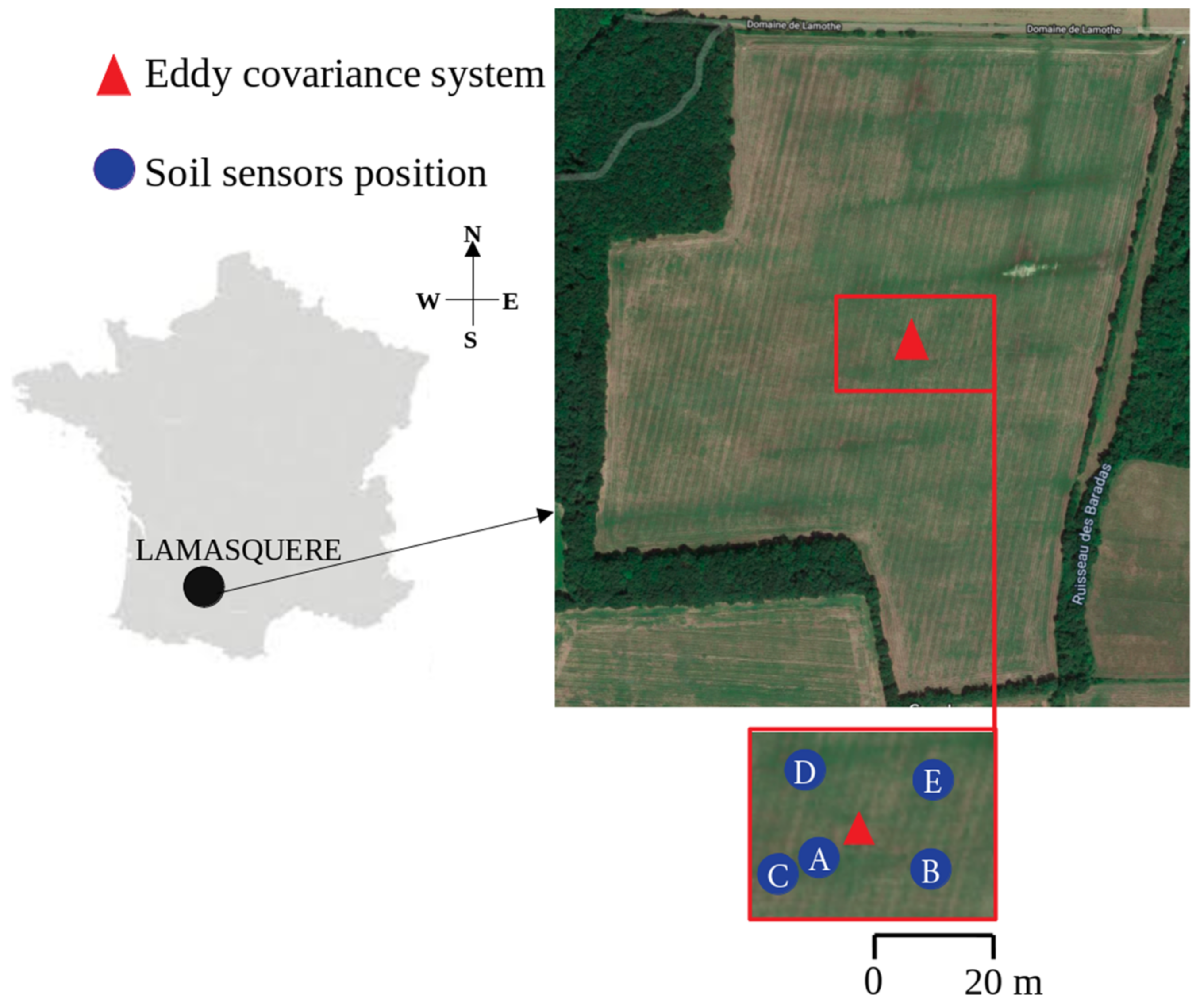
2.1. Experimental Site
2.2. Data Set Description
2.2.1. Eddy Covariance and Meteorological Measurements
2.2.2. Ground Heat Flux
2.2.3. Sap Flow Measurements
2.2.4. Vegetation Characteristics and Irrigation Water Amounts
2.2.5. Water Storage Calculation
2.2.6. Definition of Metrics
- (i)
- RMSE: Represents the root mean square deviation between the measured and the simulated variable.
- (ii)
- R2: Expresses the proportion of variance in the simulated variable that is predicted from the observed.
- (iii)
- MAE: The average magnitude of errors between the observation and the simulated datasets.
3. Model Description and Implementation
3.1. Model Description
3.2. Model Implementation
Forcing Parameter and Data
4. Results and Discussion
4.1. Experimental Data Analysis
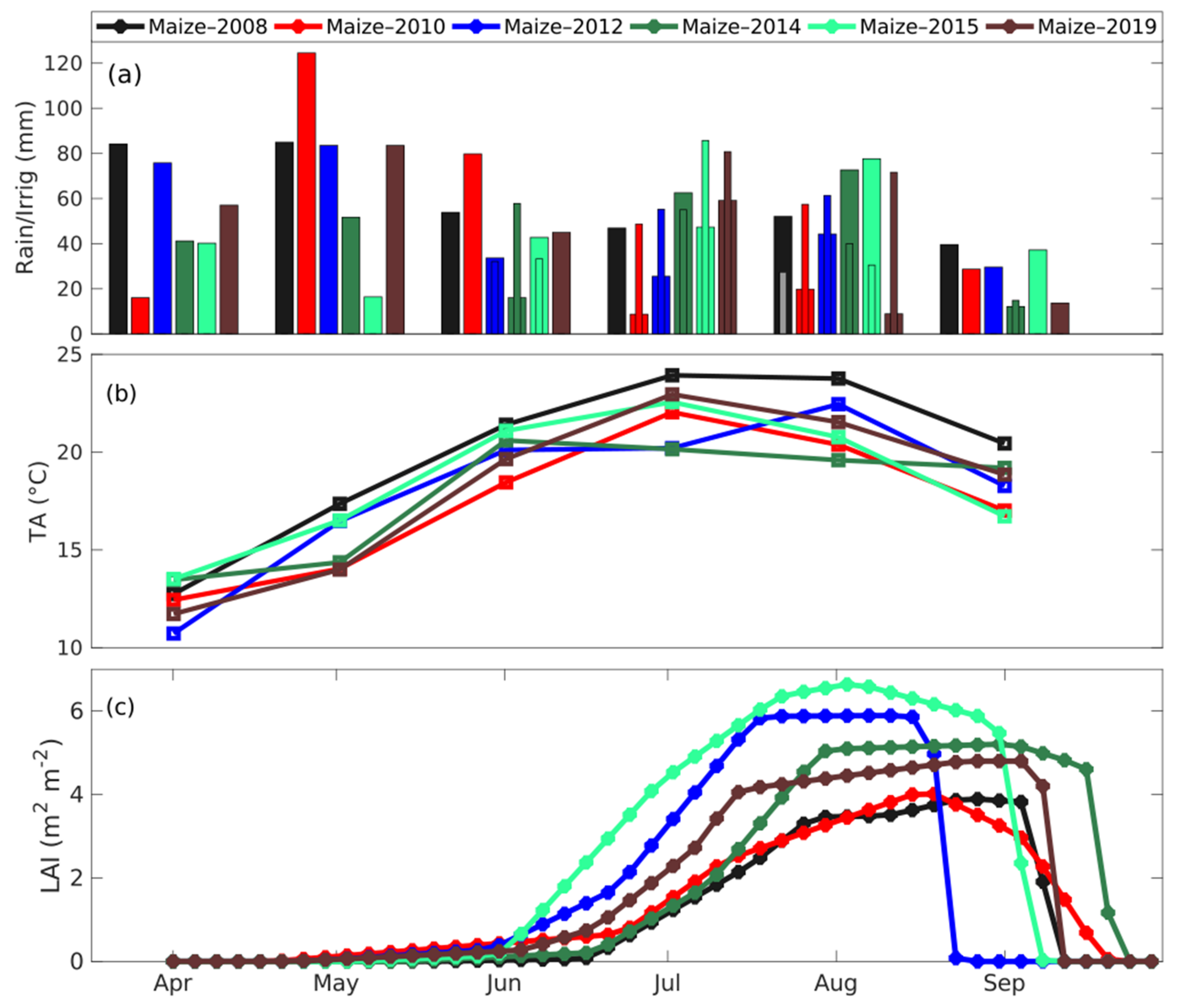
4.1.1. Meteorological Conditions and Vegetation Characteristics
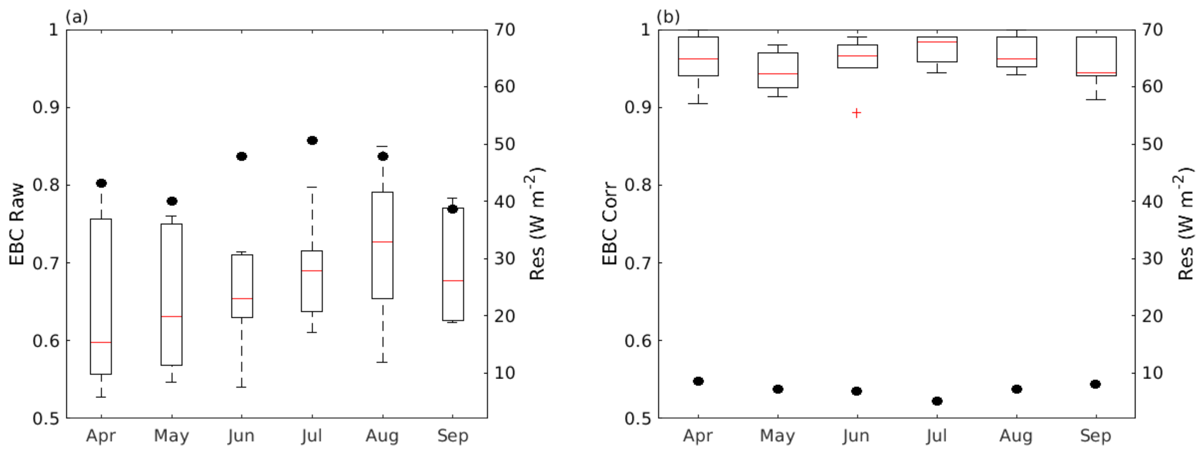
4.1.2. Energy Balance Closure
4.2. Assessment of the ISBA and ISBA-MEB Models
4.2.1. Energy Budget
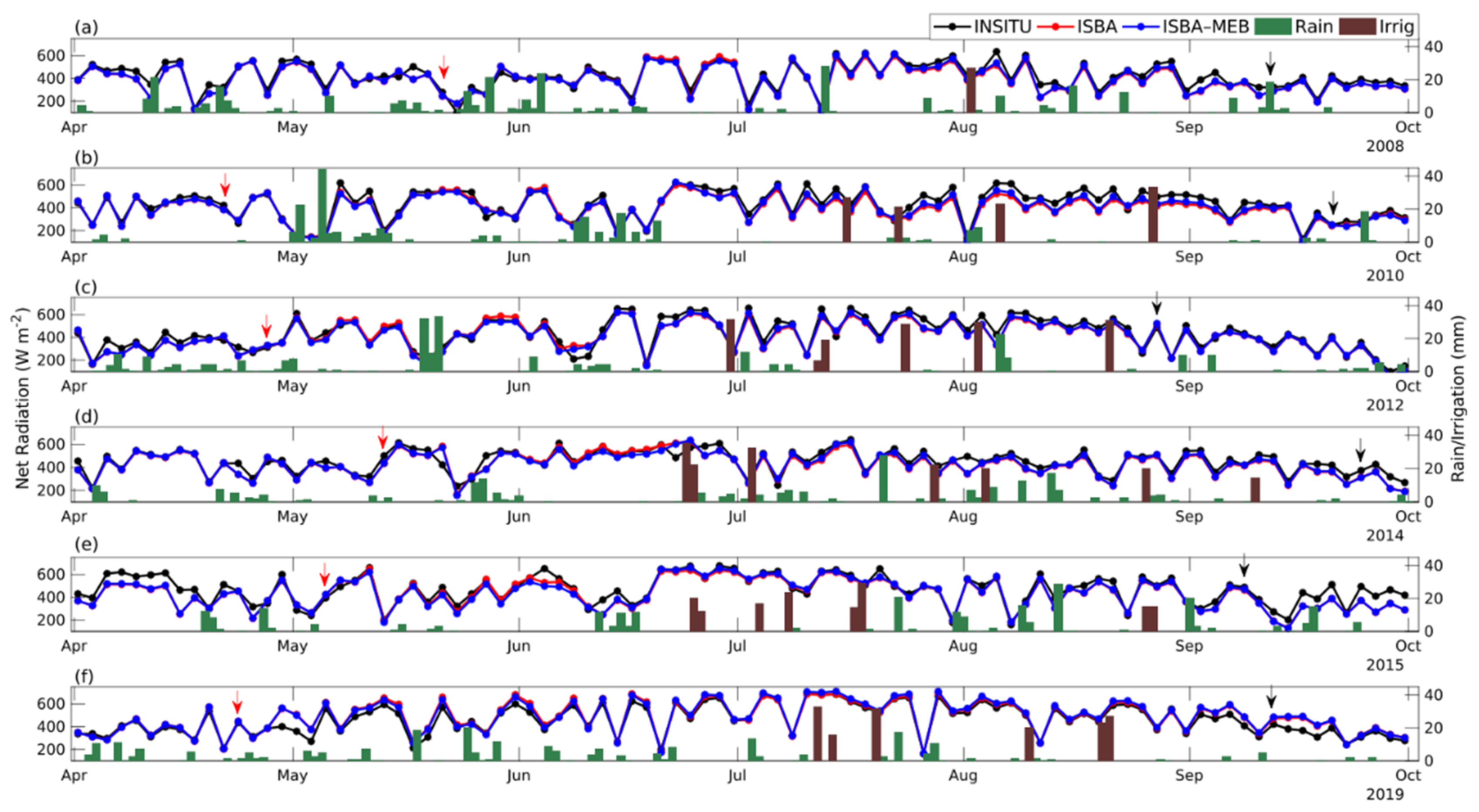
- Net radiation
- 2.
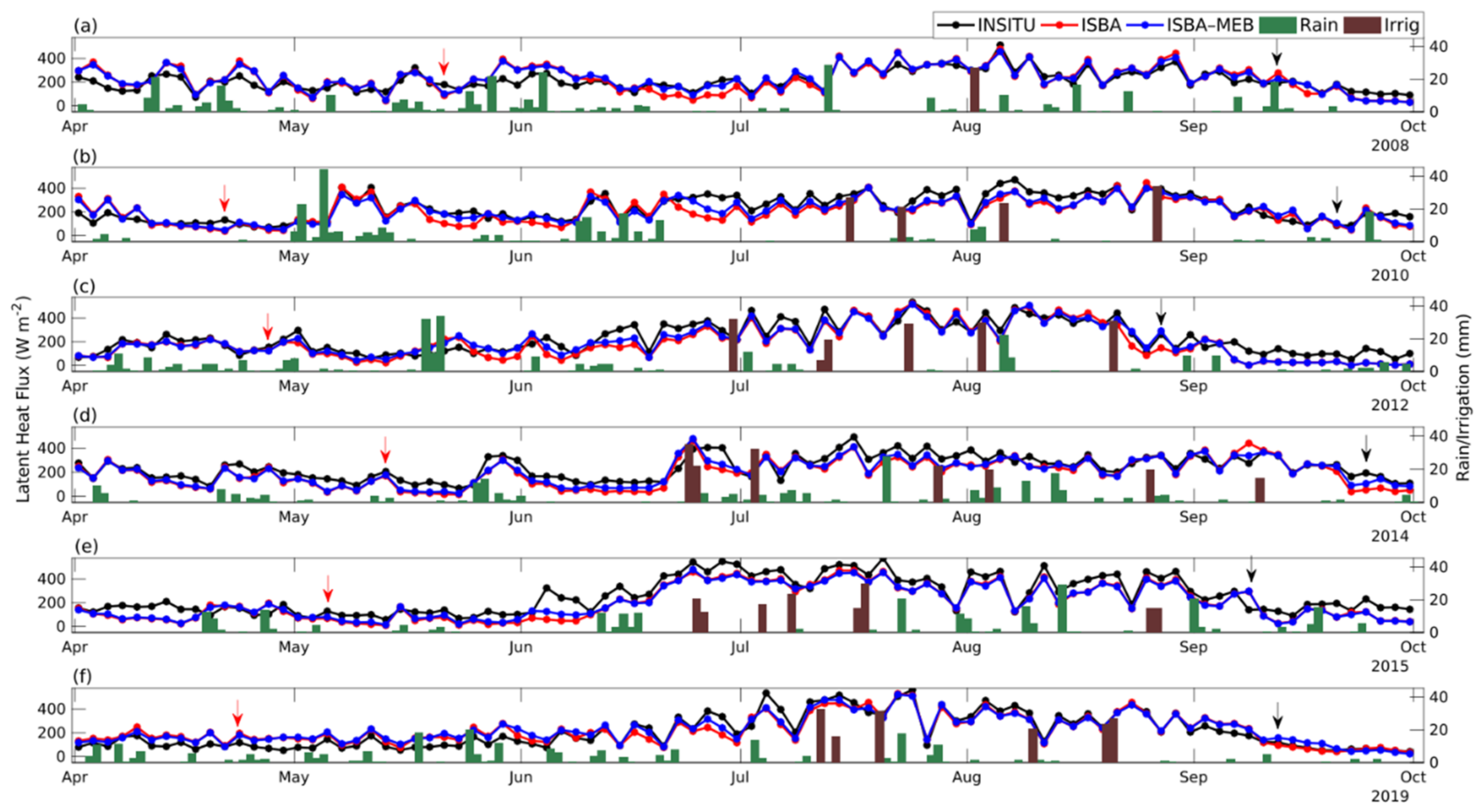
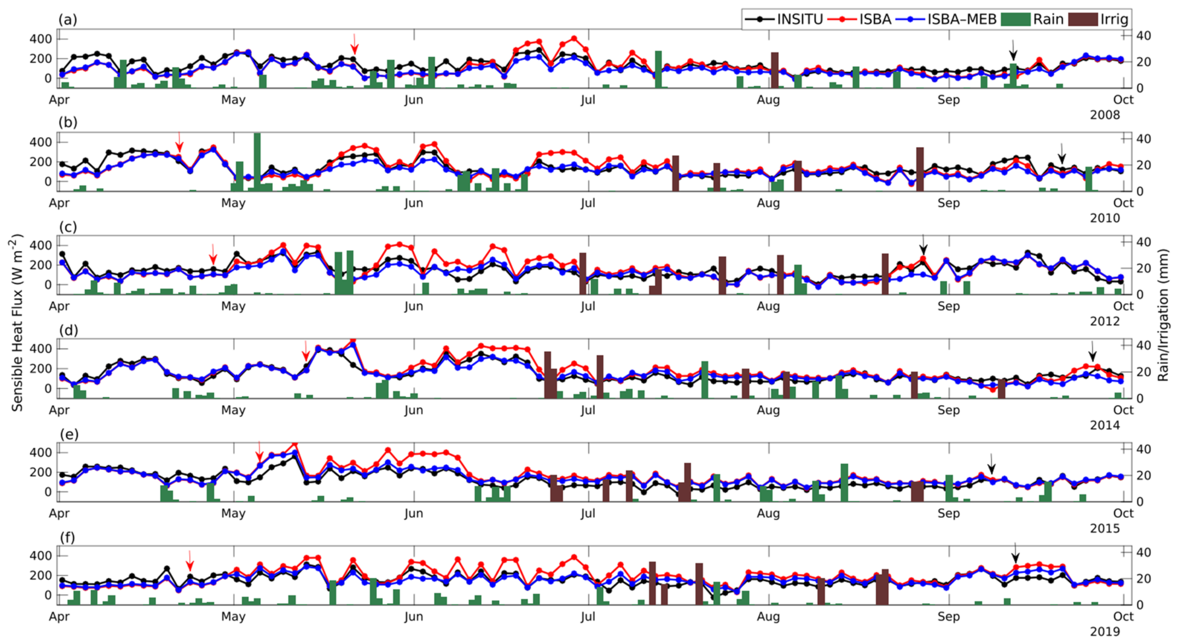
- Latent heat and sensible heat flux
- 3.
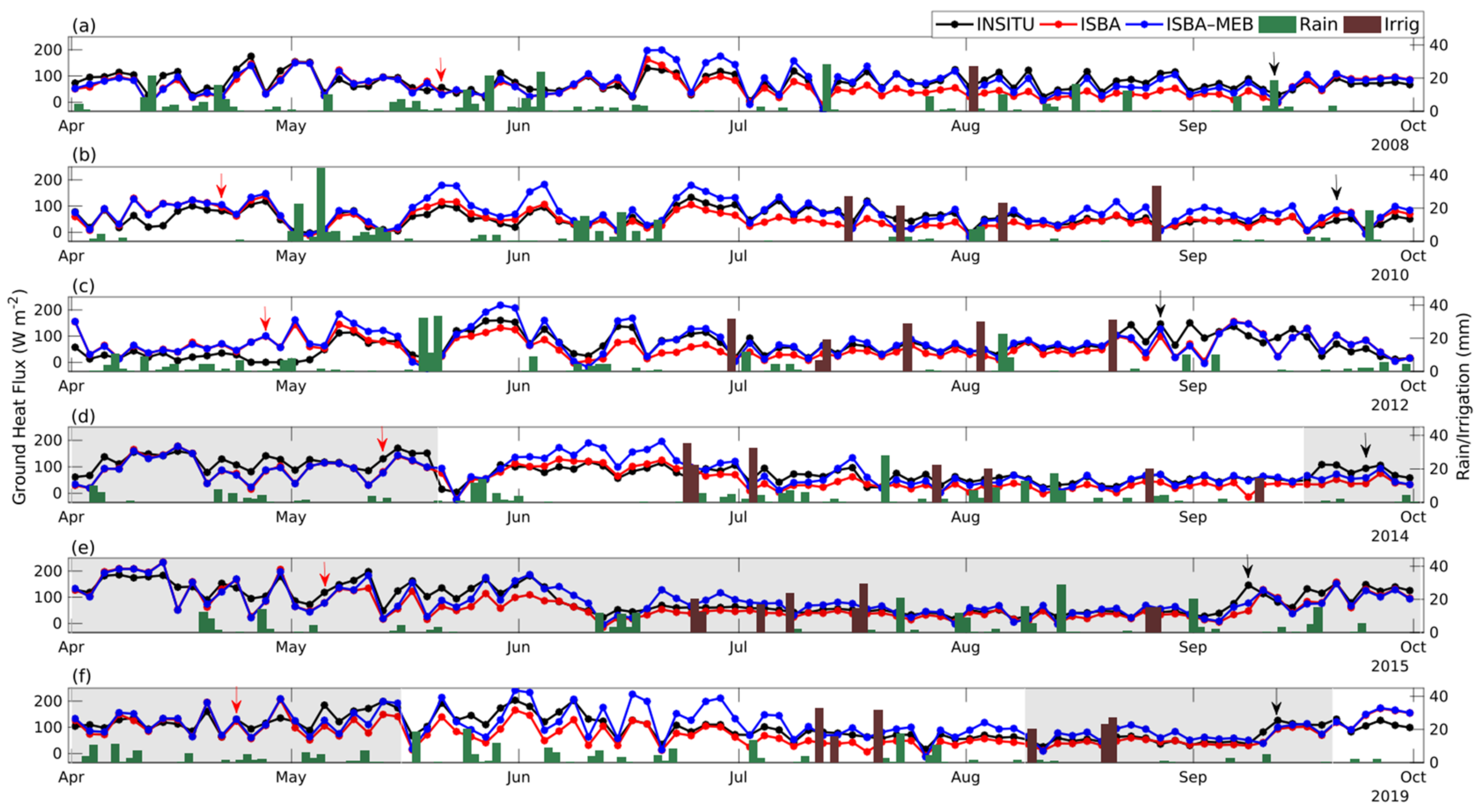
- Ground heat flux
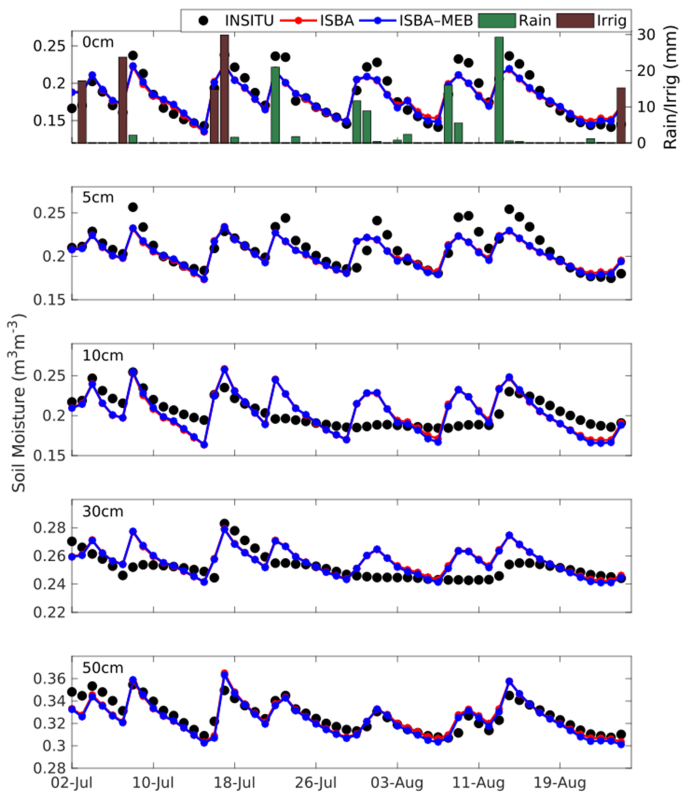
4.2.2. Soil Moisture Time Series
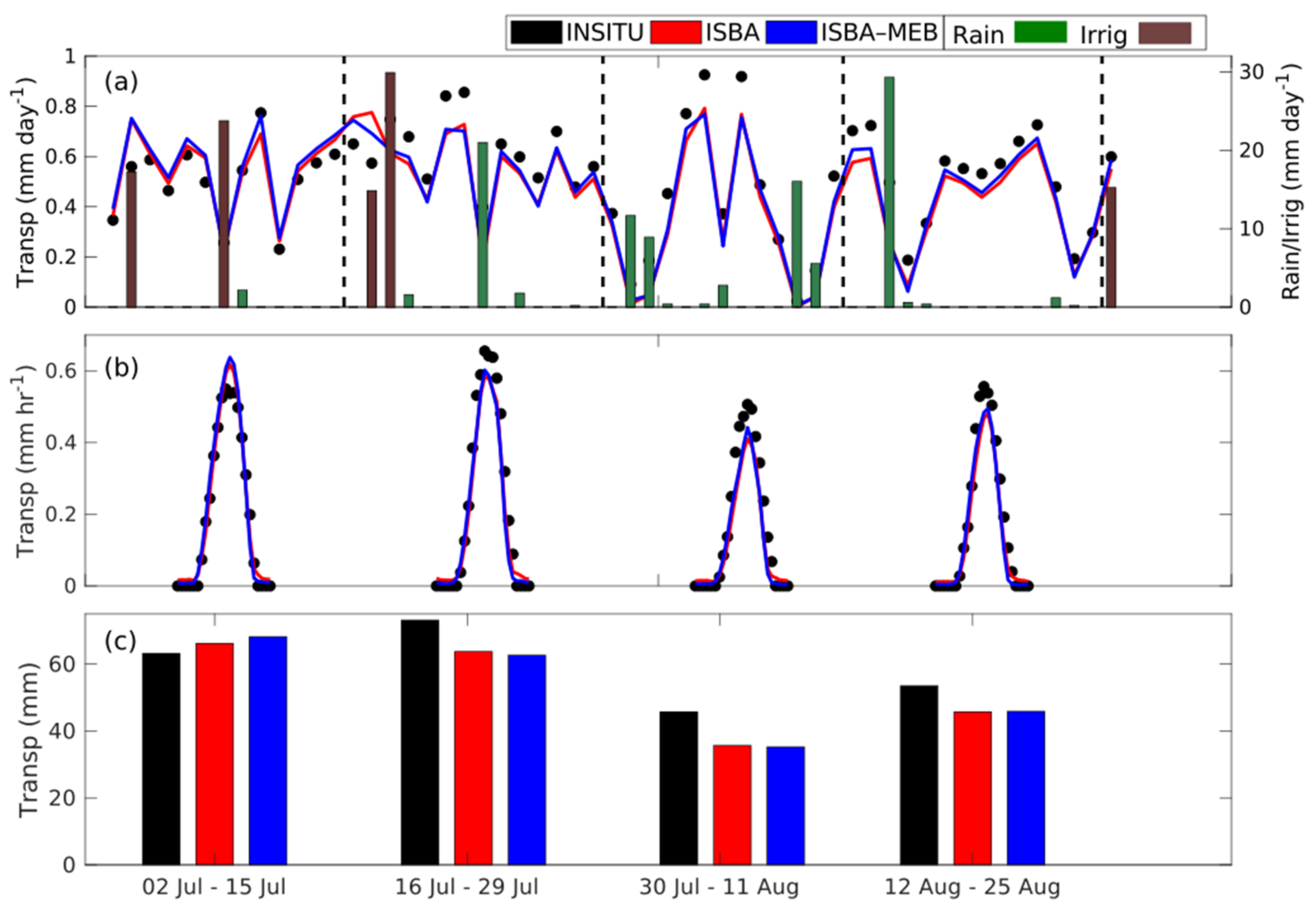
4.2.3. Transpiration
4.3. Inter-Annual Variability of Maize Water Budgets
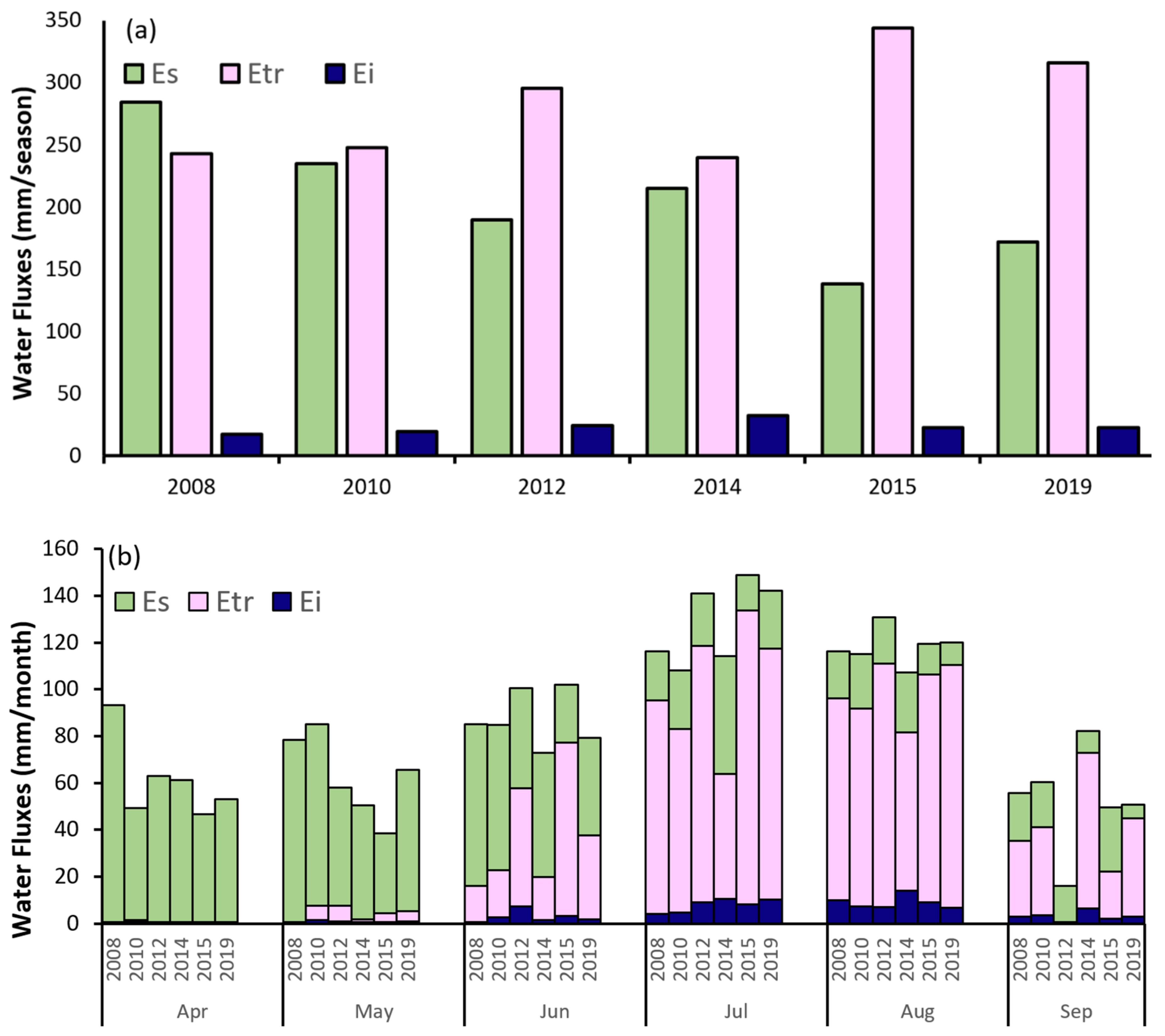
4.3.1. Evapotranspiration Partitioning
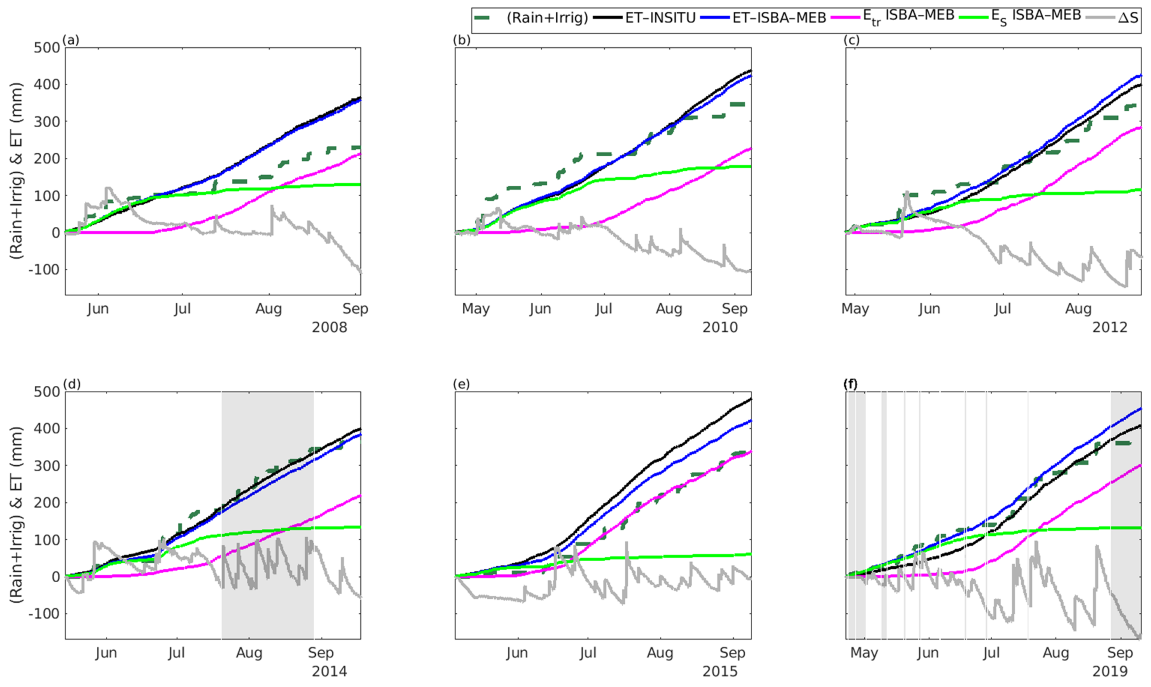
4.3.2. Maize Water Budget
5. Conclusions
- ISBA-MEB provided better estimations of the energy budget components during all the growing seasons, and the main added value of this model was in the prediction of H and to a lesser extent LE during the growth stages when the site is heterogeneous with sparse vegetation. This means that for the future projection of the hydrological functioning and water consumption of maize, a multi-energy balance approach should be preferred to single-source models.
- Concerning the evapotranspiration partition, both ISBA and ISBA-MEB showed good ability to reproduce the observed transpiration derived from sap flow measurements. Nevertheless, the campaign of these measurements took place when the canopy was fully developed, with homogeneous cover.
- On average, transpiration accounted for a large percentage of ET for most of the years: about 60% for the wet years (2012, 2014, 2015, and 2019) and 46% for the drier years (2008 and 2010). Nevertheless, the partitioning of the ET exhibited a strong year-to-year variability that was closely related to crop development measured by the LAI in this study.
- Another striking feature is that all years behave closely in terms of balance between water inputs and ET; (P + Irrig) was consistently lower than ET except in 2019, a very specific year characterized by a long period of drought in July. This is attributed to very specific conditions on our study site characterized by an existing impervious layer at around 60 cm depth that limits drainage fluxes. This impervious layer, coupled with the good irrigation practice of the farmer, precludes this study from offering recommendations on irrigation scheduling.
Supplementary Materials
Author Contributions
Funding
Data Availability Statement
Acknowledgments
Conflicts of Interest
References
- Ait-Mouheb, N.; Bahri, A.; Thayer, B.B.; Benyahia, B.; Bourrié, G.; Cherki, B.; Condom, N.; Declercq, R.; Gunes, A.; Héran, M.; et al. Mediterranean land systems under global change: Current state and future challenges. Reg. Environ. Chang. 2018, 18, 619–622. [Google Scholar] [CrossRef]
- Thornton, P.; Whitbread, A.; Baedeker, T.; Cairns, J.; Claessens, L.; Baethgen, W.; Keating, B. A framework for priority-setting in climate smart agriculture research. Agric. Syst. 2018, 167, 161–175. [Google Scholar] [CrossRef]
- Ferris, R.; Wheeler, T.R.; Ellis, R.H.; Hadley, P. Seed yield after environmental stress in soybean grown under elevated CO2. Crop Sci. 1999, 39, 710–718. [Google Scholar] [CrossRef]
- Koutroulis, A.G.; Papadimitriou, L.V.; Grillakis, M.G.; Tsanis, I.K.; Warren, R.; Betts, R.A. Global water availability under high-end climate change: A vulnerability based assessment. Glob. Planet. Chang. 2019, 175, 52–63. [Google Scholar] [CrossRef]
- Schewe, J.; Heinke, J.; Gerten, D.; Haddeland, I.; Arnell, N.W.; Clark, D.B.; Dankers, R.; Eisner, S.; Fekete, B.M.; Colón-González, F.J.; et al. Multimodel assessment of water scarcity under climate change. Proc. Natl. Acad. Sci. USA 2014, 111, 3245–3250. [Google Scholar] [CrossRef] [PubMed] [Green Version]
- Bodirsky, B.L.; Rolinski, S.; Biewald, A.; Weindl, I.; Popp, A.; Lotze-Campen, H. Global food demand scenarios for the 21st century. PLoS ONE 2015, 10, e0139201. [Google Scholar] [CrossRef] [PubMed]
- Battude, M.; Al Bitar, A.; Brut, A.; Tallec, T.; Huc, M.; Cros, J.; Weber, J.; Lhuissier, L.; Simonneaux, V.; Demarez, V. Modeling water needs and total irrigation depths of maize crop in the south west of France using high spatial and temporal resolution satellite imagery. Agric. Water Manag. 2017, 189, 123–136. [Google Scholar] [CrossRef]
- Liang, X.; Lettenmaier, D.P.; Wood, E.F.; Burges, S.J. A simple hydrologically based model of land surface water and energy fluxes for general circulation models. J. Geophys. Res. 1994, 99, 14415–14428. [Google Scholar] [CrossRef]
- Koster, R.D.; Suarez, M.J. Energy and water balance calculations in the Mosaic LSM. NASA Tech. Memorandum. 1996, 104606, 60. [Google Scholar]
- Srivastava, A.; Sahoo, B.; Raghuwanshi, N.; Chatterjee, C. Modelling the dynamics of evapotranspiration using Variable Infiltration Capacity model and regionally calibrated Hargreaves approach. Irrig. Sci. 2018, 36, 289–300. [Google Scholar] [CrossRef]
- Allen, R.G.; Pereira, L.S.; Raes, D.; Smith, M. Crop evapotranspiration—Guidelines for computing crop water requirements—FAO Irrigation and drainage paper 56. Irrig. Drain. 1998, 34, 144–152. [Google Scholar] [CrossRef]
- Duchemin, B.; Hadria, R.; Erraki, S.; Boulet, G.; Maisongrande, P.; Chehbouni, A.; Escadafal, R.; Ezzahar, J.; Hoedjes, J.C.B.; Kharrou, M.H.; et al. Monitoring wheat phenology and irrigation in Central Morocco: On the use of relationships between evapotranspiration, crops coefficients, leaf area index and remotely-sensed vegetation indices. Agric. Water Manag. 2006, 79, 1–27. [Google Scholar] [CrossRef]
- Er-Raki, S.; Chehbouni, A.; Guemouria, N.; Duchemin, B.; Ezzahar, J.; Hadria, R. Combining FAO-56 model and ground-based remote sensing to estimate water consumptions of wheat crops in a semi-arid region. Agric. Water Manag. 2007, 87, 41–54. [Google Scholar] [CrossRef] [Green Version]
- Cid, P.; Taghvaeian, S.; Hansen, N.C. Evaluation of the Fao-56 Methodology for Estimating Maize Water Requirements Under Deficit and Full Irrigation Regimes in Semiarid Northeastern Colorado. Irrig. Drain. 2018, 67, 605–614. [Google Scholar] [CrossRef]
- Le Page, M.; Berjamy, B.; Fakir, Y.; Bourgin, F.; Jarlan, L.; Abourida, A.; Benrhanem, M.; Jacob, G.; Huber, M.; Sghrer, F.; et al. An Integrated DSS for Groundwater Management Based on Remote Sensing. The Case of a Semi-Arid Aquifer in Morocco. Water Resour. Manag. 2012, 26, 3209–3230. [Google Scholar] [CrossRef] [Green Version]
- Le Page, M.; Toumi, J.; Khabba, S.; Hagolle, O.; Tavernier, A.; Kharrou, M.; Er-Raki, S.; Huc, M.; Kasbani, M.; Moutamanni, A.; et al. A Life-Size and Near Real-Time Test of Irrigation Scheduling with a Sentinel-2 Like Time Series (SPOT4-Take5) in Morocco. Remote Sens. 2014, 6, 11182–11203. [Google Scholar] [CrossRef] [Green Version]
- Tramblay, Y.; Jarlan, L.; Hanich, L.; Somot, S. Future Scenarios of Surface Water Resources Availability in North African Dams. Water Resour. Manag. 2017, 32, 1291–1306. [Google Scholar] [CrossRef]
- Kalma, J.D.; McVicar, T.R.; McCabe, M.F. Estimating Land Surface Evaporation: A Review of Methods Using Remotely Sensed Surface Temperature Data. Surv. Geophys. 2008, 29, 421–469. [Google Scholar] [CrossRef]
- Norman, J.M.; Kustas, W.P.; Humes, K.S. Two Source approach for estimating soil and vegetation energy fluxes in observations of directional radiometric surface temperature. Agric. For. Meteorol. 1995, 77, 263–293. [Google Scholar] [CrossRef]
- Timmermans, W.J.; Kustas, W.P.; Anderson, M.C.; French, A.N. An intercomparison of the Surface Energy Balance Algorithm for Land (SEBAL) and the Two-Source Energy Balance (TSEB) modeling schemes. Rem. Sens. Environ. 2007, 108, 369–384. [Google Scholar] [CrossRef]
- Boulet, G.; Mougenot, B.; Lhomme, J.P.; Fanise, P.; Lili-Chabaane, Z.; Olioso, A.; Bahir, M.; Rivalland, V.; Jarlan, L.; Merlin, O.; et al. The SPARSE model for the prediction of water stress and evapotranspiration components from thermal infra-red data and its evaluation over irrigated and rainfed wheat. Hydrol. Earth Syst. Sci. 2015, 19, 4653–4672. [Google Scholar] [CrossRef] [Green Version]
- Chirouze, J.; Boulet, G.; Jarlan, L.; Fieuzal, R.; Rodriguez, J.C.; Ezzahar, J.; Er-Raki, S.; Bigeard, G.; Merlin, O.; Garatuza-Payan, J.; et al. Intercomparison of four remote-sensing-based energy balance methods to retrieve surface evapotranspiration and water stress of irrigated fields in semi-arid climate. Hydrol. Earth Syst. Sci. 2014, 18, 1165–1188. [Google Scholar] [CrossRef] [Green Version]
- Diarra, A.; Jarlan, L.; Er-Raki, S.; Le Page, M.; Aouade, G.; Tavernier, A.; Boulet, G.; Ezzahar, J.; Merlin, O.; Khabba, S. Performance of the two-source energy budget (TSEB) model for the monitoring of evapotranspiration over irrigated annual crops in North Africa. Agric. Water Manag. 2017, 193, 71–88. [Google Scholar] [CrossRef]
- Delogu, E.; Boulet, G.; Olioso, A.; Coudert, B.; Chirouze, J.; Ceschia, E.; Le Dantec, V.; Marloie, O.; Chehbouni, G.; Lagouarde, J.P. Reconstruction of temporal variations of evapotranspiration using instantaneous estimates at the time of satellite overpass. Hydrol. Earth Syst. Sci. 2012, 16, 2995–3010. [Google Scholar] [CrossRef] [Green Version]
- Coudert, B.; Ottlé, C.; Boudevillain, B.; Demarty, J.; Guillevic, P. Contribution of Thermal Infrared Remote Sensing Data in Multiobjective Calibration of a Dual-Source SVAT Model. J. Hydrometeorol. 2006, 7, 404–420. [Google Scholar] [CrossRef]
- Hurk, B.V.D.; Best, M.; Dirmeyer, P.; Pitman, A.; Polcher, J.; Santanello, J. Acceleration of land surface model development over a decade of GLASS. Am. Meteorol. Soc. 2011, 92, 1593–1600. [Google Scholar] [CrossRef] [Green Version]
- Noilhan, J.; Planton, S. A Simple Parameterization of Land Surface Processes for Meteorological Models. Mon. Weather Rev. 1989, 117, 536–549. [Google Scholar] [CrossRef]
- Sellers, P.J.; Tucker, C.J.; Collatz, G.J.; Los, S.O.; Justice, C.O.; Dazlich, D.A.; Randall, D.A. A Revised Land Surface Parameterization (SiB2) for Atmospheric GCMS. Part II: The Generation of Global Fields of Terrestrial Biophysical Parameters from Satellite Data. J. Clim. 1996, 9, 706–737. [Google Scholar] [CrossRef] [Green Version]
- Blyth, E.; Clark, D.B.; Ellis, R.; Huntingford, C.; Los, S.; Pryor, M.; Best, M.; Sitch, S. A comprehensive set of benchmark tests for a land surface model of simultaneous fluxes of water and carbon at both the global and seasonal scale. Geosci. Model Dev. 2011, 4, 255–269. [Google Scholar] [CrossRef] [Green Version]
- Blyth, E.; Gash, J.; Lloyd, A.; Pryor, M.; Weedon, G.P.; Shuttleworth, J. Evaluating the JULES land surface model energy fluxes using FLUXNET data. J. Hydrometeorol. 2010, 11, 509–519. [Google Scholar] [CrossRef] [Green Version]
- Boone, A.; De Rosnay, P.; Balsamo, G.; Beljaars, A.; Chopin, F.; Decharme, B.; Delire, C.; Ducharne, A.; Gascoin, S.; Grippa, M.; et al. The AMMA land surface model intercomparison project (ALMIP). Bull. Am. Meteorol. Soc. 2009, 90, 1865–1880. [Google Scholar] [CrossRef]
- Aouade, G.; Jarlan, L.; Ezzahar, J.; Er-raki, S.; Napoly, A.; Benkaddour, A.; Khabba, S.; Boulet, G.; Garrigues, S.; Chehbouni, A.; et al. Evapotranspiration partition using the multiple energy balance version of the ISBA-A-gs; land surface model over two irrigated crops in a semi-arid Mediterranean region (Marrakech, Morocco). Hydrol. Earth Syst. Sci. 2019, 24, 3789–3814. [Google Scholar] [CrossRef]
- Garrigues, S.; Olioso, A.; Calvet, J.C.; Martin, E.; Lafont, S.; Moulin, S.; Chanzy, A.; Marloie, O.; Buis, S.; Desfonds, V.; et al. Evaluation of land surface model simulations of evapotranspiration over a 12-year crop succession: Impact of soil hydraulic and vegetation properties. Hydrol. Earth Syst. Sci. 2015, 19, 3109–3131. [Google Scholar] [CrossRef] [Green Version]
- Novick, K.; Biederman, J.; Desai, A.; Litvak, M.; Moore, D.; Scott, R.; Torn, M. The AmeriFlux network: A coalition of the willing. Agric. For. Meteorol. 2017, 249, 444–456. [Google Scholar] [CrossRef] [Green Version]
- Beringer, J.; Hutley, L.B.; McHugh, I.; Arndt, S.K.; Campbell, D.; Cleugh, H.A.; Cleverly, J.; Resco de Dios, V.; Eamus, D.; Evans, B.; et al. An introduction to the Australian and New Zealand flux tower network–OzFlux. Biogeosciences 2016, 13, 5895–5916. [Google Scholar] [CrossRef] [Green Version]
- Baldocchi, D.; Falge, E.; Gu, L.; Olson, R.; Hollinger, D.; Running, S.; Anthoni, P.; Bernhofer, C.; Davis, K.; Evans, R. FLUXNET: A new tool to study the temporal and spatial variability of ecosystem-scale carbon dioxide, water vapor, and energy flux densities. Bull. Amer. Meteor. Soc. 2001, 82, 2415–2434. [Google Scholar] [CrossRef]
- McDermid, S.S.; Mearns, L.O.; Ruane, A.C. Representing agriculture in Earth System Models: Approaches and priorities for development. J. Adv. Model. Earth Syst. 2017, 9, 2230–2265. [Google Scholar] [CrossRef]
- Pitman, A.J. The evolution of, and revolution in, land surface schemes designed for climate models. Int. J. Climatol. 2003, 23, 479–510. [Google Scholar] [CrossRef]
- Viterbo, P. A Review of Parametrization Schemes for Land Surface Processes. Meteorol. Train. Course Lect. Ser., 49.Eur Cent. For Med.-Range Weather Forecasts, Reading, U.K. 2002. Available online: http://www.dca.ufcg.edu.br/mna/Anexo-MNA-modulo03d.pdf (accessed on 23 May 2021).
- Blyth, E.M.; Harding, R.J. Application of aggregation models to surface heat flux from the Sahelian tiger bush. Agric. For. Meteorol. 1995, 72, 213–235. [Google Scholar] [CrossRef]
- Boulet, G.; Chehbouni, A.; Braud, I.; Vauclin, M. Mosaic versus dual source approaches for modelling the surface energy balance of a semi-arid land. Hydrol. Earth Syst. Sci. 1999, 3, 247–258. [Google Scholar] [CrossRef]
- Balsamo, G.; Pappenberger, F.; Dutra, E.; Viterbo, P.; Van den Hurk, B. A revised land hydrology in the ECMWF model: A step towards daily water flux prediction in a fully-closed water cycle. Hydrol. Process. 2011, 25, 1046–1054. [Google Scholar] [CrossRef]
- Van Hurk, B.J.J.M.D.; Verhoef, A.; Van Berg, A.R.D.; De Bruin, H.A.R. An intercomparison of three vegetation/soil models for a sparse vineyard canopy. Q. J. R. Meteorol. Soc. 1995, 121, 1867–1889. [Google Scholar] [CrossRef]
- Boone, A.; Samuelsson, P.; Gollvik, S.; Napoly, A.; Jarlan, L.; Brun, E.; Decharme, B. The interactions between soil-biosphere-atmosphere land surface model with a multi-energy balance (ISBA–MEB) option in SURFEXv8-Part 1: Model description. Geosci. Model Dev. 2017, 10, 843–872. [Google Scholar] [CrossRef] [Green Version]
- Sellers, P.J.; Mintz, Y.; Sud, Y.C.; Dalcher, A. A Simple Biosphere Model (SIB) for Use within General Circulation Models. J. Atmos. Sci. 1986, 43, 505–531. [Google Scholar] [CrossRef] [Green Version]
- Gaillardet, J.I.; Braud, F.; Hankard, S.; Anquetin, O.B.; Bour, O.; Dorfliger, N.; De Dreuzy, J.R.; Galle, S.; Galy, C.; Gogo, S.; et al. OZCAR: The French Network of Critical Zone Observatories. Vadose Zone. J. Soil Sci. Soc. Am. J. 2018, 17, 1–24. [Google Scholar] [CrossRef] [Green Version]
- Tallec, T.; Brut, A.; Joly, L.; DumeliÃc, N.; Serça, D.; Mordelet, P.; Le Dantec, V. N2O flux measurements over an irrigated maize crop: A comparison of three methods. Agric. For. Meteorol. 2019, 264, 56–72. [Google Scholar] [CrossRef]
- Béziat, P.; Rivalland, V.; Tallec, T.; Jarosz, N.; Boulet, G.; Gentine, P.; Ceschia, E. Evaluation of a simple approach for crop evapotranspiration partitioning and analysis of the water budget distribution for several crop species. Agric. For. Meteorol. 2013, 177, 46–56. [Google Scholar] [CrossRef] [Green Version]
- Falge, E.; Baldocchi, D.; Olson, R.; Anthoni, P.; Aubinet, M.; Bernhofer, C.; Burba, G.; Ceulemans, R.; Clement, R.; Dolman, H.; et al. Gap filling strategies for long term energy flux data sets. Agric. For. Meteorol. 2001, 107, 71–77. [Google Scholar] [CrossRef] [Green Version]
- Moffat, A.M.; Papale, D.; Reichstein, M.; Hollinger, D.Y.; Richardson, A.D.; Barr, A.G.; Beckstein, C.; Braswell, B.H.; Churkina, G.; Desai, A.R.; et al. Comprehensive comparison of gap-filling techniques for eddy covariance net carbon fluxes. Agric. For. Meteorol. 2007, 147, 209–232. [Google Scholar] [CrossRef]
- Mauder, M.; Foken, T.; Clement, R.; Elbers, J.A.; Eugster, W.; Grünwald, T.; Heusinkveld, B.; Kolle, O. Quality control of CarboEurope flux data—Part 2: Inter-comparison of eddy-covariance software. Biogeosciences 2008, 5, 451–462. [Google Scholar] [CrossRef] [Green Version]
- Meyers, T.; Hollinger, S. An assessment of storage terms in the surface energy balance of maize and soybean. Agric. For. Meteorol. 2004, 125, 105–115. [Google Scholar] [CrossRef]
- Miralles, D.G.; Holmes, T.R.H.; De Jeu, R.A.M.; Gash, J.H.; Meesters, A.G.C.A.; Dolman, A.J. Global land-surface evapotranspiration estimated from satellite-based observations. Hydrol. Earth Syst. Sci. 2011, 15, 453–469. [Google Scholar] [CrossRef] [Green Version]
- Tasumi, M. Progress in Operational Estimation of Regional Evapotranspiration Using Satellite Imagery. Ph.D. Thesis, University of Idaho, Moscow, ID, USA, 2003. [Google Scholar]
- Choudhury, B.J.; Idso, S.B.; Reginato, R.J. Analysis of an empirical model for soil heat flux under a growing wheat crop for estimating evaporation by an infrared-temperature based energy balance equation. Agric. For. Meteorol. 1987, 39, 283–297. [Google Scholar] [CrossRef]
- Sakuratani, J.; Abe, T. A heat balance method for measuring water flow rate in stems of intact plants and its application to sugarcane plants. JARQ Jpn. Agric. Res. Q. 1985, 37, 9–17. [Google Scholar] [CrossRef]
- Baker, J.M.; Van Bavel, C.H.M. Measurement of mass flow of water in the stems of herbaceous plants. Plant Cell Environ. 1987, 10, 777–782. [Google Scholar] [CrossRef]
- Claverie, M.; Demarez, V.; Duchemin, B.; Hagolle, O.; Ducrot, D.; Sicre, C.; Dejoux, J.F.; Huc, M.; Keravec, P.; Béziat, P.; et al. Maize and sunflower biomass estimation in southwest France using high spatial and temporal resolution remote sensing data. Remote Sens. Environ. 2012, 124, 844–857. [Google Scholar] [CrossRef]
- Lu, N.; Chen, S.; Wilske, B.; Sun, G.; Chen, J. Evapotranspiration and soil water relationships in a range of disturbed and undisturbed ecosystems in the semi-arid Inner Mongolia, China. J. Plant Ecol. 2011, 4, 49–60. [Google Scholar] [CrossRef] [Green Version]
- Farré, I.; Faci, J.M. Comparative response of maize (Zea mays L.) and sorghum (Sorghum bicolor L. Moench) to deficit irrigation in a Mediterranean environment. Agric. Water Mgmt. 2006, 83, 135–143. [Google Scholar] [CrossRef]
- Le Moigne, P. SURFEX Scientific Documentation. Note de Centre (CNRM/GMME); Météo-France: Toulouse, France, 2009; Volume 87, 211p. [Google Scholar]
- Calvet, J.C.; Noilhan, J.; Roujean, J.L.; Bessemoulin, P.; Cabelguenne, M.; Olioso, A.; Wigneron, J.P. An interactive vegetation SVAT model tested against data from six contrasting sites. Agric. For. Meteorol. 1998, 92, 73–95. [Google Scholar] [CrossRef]
- Calvet, J.C. Investigating soil and atmospheric plant water stress using physiological and micrometeorological data. Agric. For. Meteorol. 2000, 103, 229–247. [Google Scholar] [CrossRef]
- Jacobs, C.M.J. Direct Impact of Atmospheric CO2 Enrichment on Regional Transpiration. PhD. Thesis, Agricultural University, Wageningen, The Netherlands, 1994. [Google Scholar]
- Jacobs, C.M.J.; Van den Hurk, B.J.J.M.; De Bruin, H.A.R. Stomatal behaviour and photosynthetic rate of unstressed grapevines in semi-arid conditions. Agric. For. Meteorol. 1996, 80, 111–134. [Google Scholar] [CrossRef]
- Decharme, B.; Boone, A.; Delire, C.; Noilhan, J. Local evaluation of the Interaction between Soil-Biosphere-Atmosphere soil multilayer diffusion scheme using four pedotransfer functions. J. Geophys. Res. 2011, 116, D20. [Google Scholar] [CrossRef]
- Decharme, B.; Martin, E.; Faroux, S. Reconciling soil thermal and hydrological lower boundary conditions in land surface models. J. Geophys. Res. Atmos. 2013, 118, 7819–7834. [Google Scholar] [CrossRef]
- Deardorff, J.W. Efficient Prediction of Ground Surface Temperature and Moisture, with Inclusion of a Layer of Vegetation. J. Geophys. Res. 1978, 83, 1889–1903. [Google Scholar] [CrossRef] [Green Version]
- Garrigues, S.; Olioso, A.; Carrer, D.; Decharme, B.; Calvet, J.-C.; Martin, E.; Moulin, S.; Marloie, O. Impact of climate, vegetation, soil and crop management variables on multi-year isba-a-gs simulations of evapotranspiration over a mediterranean crop site. Geosci. Model Dev. 2015, 8, 3033–3053. [Google Scholar] [CrossRef] [Green Version]
- Napoly, A.; Boone, A.; Samuelsson, P.; Gollvik, S.; Martin, E.; Séférian, R.; Carrer, D.; Decharme, B.; Jarlan, L. The interactions between soil-biosphere-atmosphere (ISBA) land surface model multi-energy balance (MEB) option in SURFEXv8-Part 2: Introduction of a litter formulation and model evaluation for local-scale forest sites. Geosci. Model Dev. 2017, 10, 1621–1644. [Google Scholar] [CrossRef] [Green Version]
- Choudhury, B.J.; Monteith, J.L. A four-layer model for the heat budget of homogeneous land surfaces. Q. J. R. Meteorol. Soc. 1988, 114, 373–398. [Google Scholar] [CrossRef]
- Faroux, S.; Kaptué Tchuenté, A.T.; Roujean, J.L.; Masson, V.; Martin, E.; Le Moigne, P. Ecoclimap-II/Europe: A twofold database of ecosystems and surface parameters at 1 km resolution based on satellite information for use in land surface, meteorological and climate models. Geosci. Model Dev. 2013, 6, 563–582. [Google Scholar] [CrossRef] [Green Version]
- Gibelin, A.L.; Calvet, J.C.; Roujean, J.L.; Jarlan, L.; Los, S.O. Ability of the land surface model ISBA-A-gs to simulate leaf area index at the global scale: Comparison with satellites products. J. Geophys. Res. 2006, 111, D18102. [Google Scholar] [CrossRef]
- Kalma, J.D.; Stanhill, G. The radiation climate of an irrigated orange plantation. Sol. Energy 1969, 12, 491–508. [Google Scholar] [CrossRef]
- Brooks, R.H.; Corey, A.T. Properties of porous media affecting fluid flow. J. Irrig. Drain. Div. Am. Soc. Civ. Eng. 1966, 6, 61. [Google Scholar] [CrossRef]
- Clapp, R.B.; Hornberger, G.M. Empirical equations for some soil hydraulic properties. Water Resour. Res. 1978, 14, 601–604. [Google Scholar] [CrossRef] [Green Version]
- Decharme, B.; Delire, C.; Minvielle, M.; Colin, J.; Vergnes, J.P.; Alias, A.; Saint-Martin, D.; Séférian, R.; Sénési, S.; Voldoire, A. Recent changes in the ISBA-CTRIP land surface system for use in the CNRM CM6 climate model and in global offline hydrological applications. J. Adv. Model Earth Syst. 2019, 11, 1207–1252. [Google Scholar] [CrossRef]
- Anguela, T.P.; Zribi, M.; Hasenauer, S.; Habets, F.; Loumagne, C. Analysis of surface and root-zone soil moisture dynamics with ERS scatterometer and the hydrometeorological model SAFRAN-ISBA-MODCOU at Grand Morin watershed (France). Hydrol. Earth Syst. Sci. 2008, 12, 1415–1424. [Google Scholar] [CrossRef] [Green Version]
- Jackson, R.B.; Canadell, J.; Ehleringer, J.R.; Mooney, H.S.O.; Schulze, E.A. Global Analysis of Root Distributions for Terrestrial Biome. Oecologia 1996, 108, 389–411. [Google Scholar] [CrossRef]
- Culf, A.D.; Foken, T.; Gash, J.H.C. The energy balance closure problem, in vegetation, water, humans and the climate. In Vegetation, Water, Humans and the Climate: A New Perspective on an Internactive System; Kabat, P., Claussen, M., Dirmeyer, P.A., Eds.; Springer: Berlin/Heidelberg, Germany, 2004; pp. 159–166. [Google Scholar]
- Dare-Idowu, O.; Brut, A.; Cuxart, J.; Tallec, T.; Rivalland, V.; Zawilski, B.; Ceschia, E.; Jarlan, L. Surface energy balance and flux partitioning of annual crops in southwestern France. Agric. For. Meteorol 2021. under review. [Google Scholar]
- Eshonkulov, R.; Poyda, A.; Ingwersen, J.; Wizemann, H.; Weber, T.; Kremer, P.; Högy, P.; Pulatov, A.; Streck, T. Evaluating multi-year, multi-site data on the energy balance closure of eddy-covariance flux measurements at cropland sites in southwestern Germany. Biogeosciences 2019, 16, 521–540. [Google Scholar] [CrossRef] [Green Version]
- Masseroni, D.; Corbari, C.; Mancini, M. Limitations and improvements of the energy balance closure with reference to experimental data measured over a maize field. Atmósfera 2014, 27, 335–352. [Google Scholar] [CrossRef] [Green Version]
- Teixeira, A.H.; Bastiaanssen, W.G.M. Five methods to interpret field measurements of energy fluxes over a micro-sprinkler-irrigated mango orchard. Irrig. Sci. 2012, 30, 13–28. [Google Scholar] [CrossRef] [Green Version]
- Chebbi, W.; Boulet, G.; Le Dantec, V.; Chabaane, Z.; Fanise, P.; Mougenot, B.; Ayari, H. Analysis of evapotranspiration components of a rainfed olive orchard during three contrasting years in a semi-arid climate. Agric. For. Meteorol. 2018, 256, 159–178. [Google Scholar] [CrossRef]
- Ding, R.S.; Kang, S.Z.; Zhang, Y.Q.; Hao, X.M.; Tong, L.; Du, T.S. Partitioning evapotranspiration into soil evaporation and transpiration using a modified dual crop coefficient model in irrigated maize field with ground-mulching. Agric. Water Manag. 2013, 127, 85–96. [Google Scholar] [CrossRef]
- Zhou, S.; Liu, W.; Lin, W. The ratio of transpiration to evapotranspiration in a rainfed maize field on the Loess Plateau of China. Water Supply 2017, 17, 221–228. [Google Scholar] [CrossRef] [Green Version]
- Serra-Wittling, C.; Molle, B.; Chevron, B. Modernization of irrigation systems in France: What potential water savings at plot level? Revue Sci. Eaux Territ. 2020, 34, 46–53. [Google Scholar] [CrossRef]
- Nielsen, D.C.; Vigil, M.F. Soil Water Extraction for Several Dryland Crops. Agron. J. 2018, 110, 2447–2455. [Google Scholar] [CrossRef] [Green Version]


| Crop Season | Rain (mm) | Irrig (mm) | Sowing Date | Harvest Date | Max LAI (m2 m−2) |
|---|---|---|---|---|---|
| 01/04/2008–30/09/2008 | 361.6 | 27.3 | 20/05/2008 | 12/09/2008 | 3.89 |
| 01/04/2010–30/09/2010 | 277.6 | 106.1 | 21/04/2010 | 20/09/2010 | 4.01 |
| 01/04/2012–30/09/2012 | 292.5 | 148.7 | 27/04/2012 | 27/08/2012 | 5.89 |
| 01/04/2014–30/09/2014 | 256.2 | 167.7 | 14/05/2014 | 24/09/2014 | 5.21 |
| 01/04/2015–30/09/2015 | 261.5 | 149.5 | 05/05/2015 | 08/09/2015 | 6.64 |
| 01/04/2019–30/09/2019 | 267.4 | 152.4 | 22/04/2019 | 12/09/2019 | 4.8 |
| Symbol | Description | Range | Unit | References |
|---|---|---|---|---|
| fc | Vegetation fraction cover | 0–1.0 | - | Estimated |
| LAI | Leaf area index | 0–6.6 | m2 m−2 | Measured |
| hveg | Vegetation height | 0–3.3 | m | measured |
| Emissoil | Soil emissivity | 0.90 | - | - |
| Emisveg | Vegetation emissivity | 0.97 | - | - |
| albsoil | Soil albedo | 0.12–0.16 | - | Derived from measurement |
| albveg | Vegetation albedo | 0.17–0.28 | - | Derived from measurement |
| Cl | Sand fraction | 0.10–0.12 | - | measured |
| Sd | Clay fraction | 0.48–0.53 | - | measured |
| gm | Mesophyll conductance | 0.0020 | m s−1 | [63]; Table 1 |
| Γ | Coefficient for the calculation of the surface stomatal resistance | 0.02 | [63]; Table 1 | |
| Wrmax | Coefficient for maximum interception water storage capacity | 0.2 | [27]; Equation (24) | |
| Cv | Thermal coefficient for the vegetation canopy | 0.00005 | K m2 J−1 | [27]; Equation (8) |
| gc | Cuticular conductance | 0.0004 | m s−1 | [73] |
| Θc | Critical normalized soil water content for stress parameterization | 0.334 | - | [63]; Equation (9) |
| Dmax | Maximum air saturation deficit | 0.065 | kg kg−1 | [63]; Equation (A3) |
| Layer (cm) | Clay (%) | Sand (%) | CONDSAT | MPOTSAT | BCOEF | WP (m3 m−3) | FC (m3 m−3) | SAT (m3 m−3) |
|---|---|---|---|---|---|---|---|---|
| 0 | 51 | 12 | 0.0000001081 | −0.5551 | 10.488 | 0.1052 | 0.2520 | 0.2913 |
| 5 | 52 | 11 | 0.0000001067 | −0.5665 | 10.625 | 0.1062 | 0.2550 | 0.2924 |
| 10 | 53 | 10 | 0.0000001057 | −0.5781 | 10.762 | 0.1152 | 0.2556 | 0.2933 |
| 30 | 50 | 11 | 0.0000001088 | −0.5665 | 10.351 | 0.1045 | 0.2420 | 0.2933 |
| 50 | 48 | 11 | 0.0000001120 | −0.5665 | 10.077 | 0.1033 | 0.2289 | 0.4222 |
| Maize Year | Model | Indicator | Rn | LE | H | G |
|---|---|---|---|---|---|---|
| 2008 | ISBA | R2 | 0.97 | 0.81 | 0.67 | 0.75 |
| RMSE | 34.0 | 56.0 | 42.9 | 37.1 | ||
| MAE | 25.0 | 33.9 | 27.5 | 26.6 | ||
| ISBA-MEB | R2 | 0.98 | 0.83 | 0.73 | 0.81 | |
| RMSE | 33.5 | 50.7 | 30.2 | 32.1 | ||
| MAE | 27.5 | 31.7 | 25.9 | 27.1 | ||
| 2010 | ISBA | R2 | 0.98 | 0.81 | 0.73 | 0.81 |
| RMSE | 33.4 | 46.9 | 45.1 | 28.8 | ||
| MAE | 22.1 | 31.8 | 29.9 | 21.5 | ||
| ISBA-MEB | R2 | 0.98 | 0.84 | 0.77 | 0.89 | |
| RMSE | 32.2 | 42.2 | 31.2 | 21.7 | ||
| MAE | 22.6 | 29.7 | 27.1 | 26.9 | ||
| 2012 | ISBA | R2 | 0.96 | 0.77 | 0.66 | 0.74 |
| RMSE | 42.7 | 58.9 | 58.5 | 26.7 | ||
| MAE | 27.5 | 36.1 | 39.3 | 34.7 | ||
| ISBA-MEB | R2 | 0.96 | 0.80 | 0.68 | 0.86 | |
| RMSE | 41.7 | 53.2 | 43.3 | 19.8 | ||
| MAE | 28.2 | 34.0 | 34.3 | 43.2 | ||
| 2014 | ISBA | R2 | 0.96 | 0.79 | 0.78 | 0.73 |
| RMSE | 46.6 | 50.9 | 47.4 | 38.1 | ||
| MAE | 28.3 | 31.5 | 34.5 | 29.7 | ||
| ISBA-MEB | R2 | 0.96 | 0.85 | 0.80 | 0.79 | |
| RMSE | 46.7 | 42.7 | 37.6 | 41.1 | ||
| MAE | 29.4 | 28.1 | 30.6 | 32.9 | ||
| 2015 | ISBA | R2 | 0.97 | 0.87 | 0.70 | 0.76 |
| RMSE | 40.6 | 43.1 | 51.8 | 41.9 | ||
| MAE | 29.5 | 34.1 | 45.8 | 39.7 | ||
| ISBA-MEB | R2 | 0.97 | 0.88 | 0.72 | 0.79 | |
| RMSE | 39.7 | 39.6 | 41.8 | 44.8 | ||
| MAE | 29.9 | 33.0 | 40.9 | 48.5 | ||
| 2019 | ISBA | R2 | 0.96 | 0.85 | 0.76 | 0.76 |
| RMSE | 44.2 | 44.3 | 47.6 | 37.4 | ||
| MAE | 30.1 | 26.7 | 33.7 | 36.7 | ||
| ISBA-MEB | R2 | 0.96 | 0.88 | 0.78 | 0.82 | |
| RMSE | 43.0 | 38.9 | 34.2 | 41.5 | ||
| MAE | 31.7 | 26.3 | 28.1 | 48.3 |
| Year | Indicator | Model | 0 cm | 5 cm | 10 cm | 30 cm | 50 cm | 100 cm |
|---|---|---|---|---|---|---|---|---|
| 2008 | R2 | ISBA | - | 0.77 | 0.80 | 0.71 | - | 0.30 |
| ISBA-MEB | - | 0.77 | 0.79 | 0.75 | - | 0.30 | ||
| RMSE | ISBA | - | 0.024 | 0.021 | 0.019 | - | 0.029 | |
| ISBA-MEB | - | 0.026 | 0.023 | 0.019 | - | 0.032 | ||
| MAE | ISBA | - | 0.026 | 0.032 | 0.053 | - | 0.060 | |
| ISBA-MEB | - | 0.029 | 0.037 | 0.056 | - | 0.062 | ||
| 2010 | R2 | ISBA | - | 0.60 | 0.71 | 0.46 | - | 0.40 |
| ISBA-MEB | - | 0.59 | 0.76 | 0.51 | - | 0.39 | ||
| RMSE | ISBA | - | 0.033 | 0.024 | 0.022 | - | 0.022 | |
| ISBA-MEB | - | 0.035 | 0.024 | 0.023 | - | 0.025 | ||
| MAE | ISBA | - | 0.027 | 0.019 | 0.037 | - | 0.035 | |
| ISBA-MEB | - | 0.029 | 0.020 | 0.038 | - | 0.037 | ||
| 2012 | R2 | ISBA | 0.40 | 0.59 | 0.40 | 0.30 | 0.91 | 0.32 |
| ISBA-MEB | 0.40 | 0.63 | 0.49 | 0.30 | 0.89 | 0.31 | ||
| RMSE | ISBA | 0.060 | 0.032 | 0.032 | 0.025 | 0.019 | 0.027 | |
| ISBA-MEB | 0.062 | 0.034 | 0.034 | 0.025 | 0.023 | 0.033 | ||
| MAE | ISBA | 0.059 | 0.031 | 0.039 | 0.025 | 0.065 | 0.045 | |
| ISBA-MEB | 0.064 | 0.033 | 0.04 | 0.025 | 0.079 | 0.052 | ||
| 2014 | R2 | ISBA | 0.42 | 0.42 | 0.68 | 0.33 | 0.73 | 0.38 |
| ISBA-MEB | 0.46 | 0.40 | 0.76 | 0.36 | 0.77 | 0.47 | ||
| RMSE | ISBA | 0.046 | 0.018 | 0.024 | 0.015 | 0.011 | 0.008 | |
| ISBA-MEB | 0.049 | 0.019 | 0.023 | 0.015 | 0.012 | 0.008 | ||
| MAE | ISBA | 0.037 | 0.027 | 0.024 | 0.022 | 0.027 | 0.016 | |
| ISBA-MEB | 0.039 | 0.026 | 0.025 | 0.022 | 0.032 | 0.019 | ||
| 2015 | R2 | ISBA | 0.65 | 0.57 | 0.30 | 0.30 | 0.48 | 0.69 |
| ISBA-MEB | 0.71 | 0.64 | 0.30 | 0.26 | 0.51 | 0.69 | ||
| RMSE | ISBA | 0.031 | 0.021 | 0.031 | 0.017 | 0.013 | 0.007 | |
| ISBA-MEB | 0.023 | 0.022 | 0.032 | 0.029 | 0.016 | 0.010 | ||
| MAE | ISBA | 0.027 | 0.017 | 0.045 | 0.033 | 0.011 | 0.013 | |
| ISBA-MEB | 0.036 | 0.018 | 0.043 | 0.030 | 0.015 | 0.017 | ||
| 2019 | R2 | ISBA | 0.31 | 0.46 | 0.53 | 0.41 | 0.62 | 0.58 |
| ISBA-MEB | 0.30 | 0.45 | 0.54 | 0.41 | 0.67 | 0.57 | ||
| RMSE | ISBA | 0.043 | 0.036 | 0.014 | 0.023 | 0.023 | 0.012 | |
| ISBA-MEB | 0.045 | 0.038 | 0.017 | 0.026 | 0.043 | 0.016 | ||
| MAE | ISBA | 0.046 | 0.033 | 0.026 | 0.023 | 0.034 | 0.031 | |
| ISBA-MEB | 0.051 | 0.036 | 0.024 | 0.025 | 0.036 | 0.036 |
| Model | R2 | RMSE (mm h−1) | MAE (mm h−1) |
|---|---|---|---|
| ISBA | 0.90 | 0.074 | 0.052 |
| ISBA-MEB | 0.91 | 0.071 | 0.048 |
| Year | 2008 | 2010 | 2012 | 2014 | 2015 | 2019 |
|---|---|---|---|---|---|---|
| P + Irrig | 229.1 | 347.9 | 343.9 | 362.7 | 333.8 | 368.1 |
| ETINSITU | 366.2 | 439.2 | 399.7 | 400.8 | 477.5 | 408.5 |
| EtrISBA-MEB | 214.1 | 227.5 | 288.8 | 220.4 | 342.5 | 302.0 |
| ESISBA-MEB | 129.7 | 180.1 | 116.8 | 134.1 | 60.9 | 131.9 |
| ΔS | 109.2 | 103.8 | 68.2 | 58.3 | 61.5 | 136.2 |
| D | −27.9 | 12.5 | 11.4 | 20.2 | −82.2 | 95. |
Publisher’s Note: MDPI stays neutral with regard to jurisdictional claims in published maps and institutional affiliations. |
© 2021 by the authors. Licensee MDPI, Basel, Switzerland. This article is an open access article distributed under the terms and conditions of the Creative Commons Attribution (CC BY) license (https://creativecommons.org/licenses/by/4.0/).
Share and Cite
Dare-Idowu, O.; Jarlan, L.; Le-Dantec, V.; Rivalland, V.; Ceschia, E.; Boone, A.; Brut, A. Hydrological Functioning of Maize Crops in Southwest France Using Eddy Covariance Measurements and a Land Surface Model. Water 2021, 13, 1481. https://doi.org/10.3390/w13111481
Dare-Idowu O, Jarlan L, Le-Dantec V, Rivalland V, Ceschia E, Boone A, Brut A. Hydrological Functioning of Maize Crops in Southwest France Using Eddy Covariance Measurements and a Land Surface Model. Water. 2021; 13(11):1481. https://doi.org/10.3390/w13111481
Chicago/Turabian StyleDare-Idowu, Oluwakemi, Lionel Jarlan, Valerie Le-Dantec, Vincent Rivalland, Eric Ceschia, Aaron Boone, and Aurore Brut. 2021. "Hydrological Functioning of Maize Crops in Southwest France Using Eddy Covariance Measurements and a Land Surface Model" Water 13, no. 11: 1481. https://doi.org/10.3390/w13111481