
A GIS-Based Hydrological Modeling Approach for Rapid Urban Flood Hazard Assessment
by
 , ,
, ,
Qianqian Zhou
1,* ,
,
Jiongheng Su
2,
Karsten Arnbjerg-Nielsen
3,
Yi Ren
4,
Jinhua Luo
1,
Zijian Ye
1 and
Junman Feng
1 1
School of Civil and Transportation Engineering, Guangdong University of Technology, Waihuan Xi Road, Guangzhou 510006, China
2
Guangdong Urban & Rural Planning and Design Institute, No.483 Nanzhou Road, Guangzhou 510290, China
3
Department of Environmental Engineering (DTU Environment), Technical University of Denmark, Miljøvej, Building 113, DK-2800 Lyngby, Denmark
4
China Water Resources Pearl River Planning Surveying & Designing Co., Ltd., No. 19 Zhanyizhi Street, Tianshou Road, Guangzhou 510610, China
*
Author to whom correspondence should be addressed.
Water 2021, 13(11), 1483; https://doi.org/10.3390/w13111483
Submission received: 15 April 2021
/
Revised: 19 May 2021
/
Accepted: 20 May 2021
/
Published: 25 May 2021
(This article belongs to the Special Issue GIS Application: Flood Risk Management)
Abstract
:Urban floods are detrimental to societies, and flood mapping techniques provide essential support for decision-making on the better management of flood risks. This study presents a GIS-based flood characterization methodology for the rapid and efficient identification of urban flood-prone areas, which is especially relevant for large-scale flood hazards and emergency assessments for data-scarce studies. The results suggested that optimal flood mapping was achieved by adopting the median values of the thresholds for local depression extraction, the topographic wetness index (TWI) and aggregation analyses. This study showed the constraints of the depression extraction and TWI methods and proposed a methodology to improve the performance. A new performance indicator was further introduced to improve the evaluation ability of hazard mapping. It was shown that the developed methodology has a much lower demand on the data and computation efforts in comparison to the traditional two-dimensional models and, meanwhile, provides relatively accurate and robust assessments of flood hazards.
1. Introduction
Urban flooding is one of the most frequent and severe natural disasters, exerting tremendous impacts on the economy, society and environment [1,2,3]. In recent years, climate change has greatly affected the hydrological cycle and patterns of precipitation and has led to increasing amounts of surface runoffs and urban floods [4,5]. On the other hand, rapid urbanization contributes to increasing impervious surfaces and has impacts on both flood hazards and vulnerability due to changes in the population, wealth and infrastructure [6,7]. Flood risks in many regions are rising and result in great damages [8,9]. During 1995–2015, 2.3 billion people were affected by floods, with total damage losses of $662 billion worldwide [10]. A flood hazard assessment can provide important information for decision-makers to better understand the flood risk and, further, strategically reduce flood losses [11,12,13,14,15].
The flood hazard assessment tools mainly include Geographic Information System (GIS)-based hydrological analysis models [16,17], one-dimensional (1D) hydrodynamic models [18,19], dual one-dimensional (1D/1D) models [20,21] and 1D/2D-coupled models [22,23]. GIS-based models can be employed to quickly capture the local depressions, main flow paths and overland discharge/accumulations. However, basic GIS tools are often associated with low accuracy and fail to take into account the interactions between sewer systems and surface runoffs [24]. The 1D models have the advantages of a high calculation efficiency and reliability for pipe network analysis; however, they are incapable of performing surface inundation calculations [25,26]. The coupled 1D/2D models can realize the surface routing calculation and simulate the interactions between the sewer and surface, with advantages in the simulation accuracy and dynamic process description. Nevertheless, the 2D calculations require huge effort on both the data processing and computational demands [26,27]. In recent years, the 1D/1D models have been developed as they pursue a balance between efficiency and accuracy, which are preferable under the circumstances of an emergency assessment and data insufficiency [28,29]. It should be noted that, for the dual 1D model, the characterization quality of the surface can have an impact on the precision of flood simulation. There is also a high demand on data to interpret 2D flow into a 1D simulation [30].
Despite the advances in flood hazard mapping tools and computational resources, high-quality flood mapping remains challenging for studies with a large analysis scale, limited evaluation time and scarce data conditions. An increasing number of scholars have explored ways of rapid hazard mapping. Chen et al. [31] adopted a multilayered approach for flood mapping to improve the accuracy of coarse grid modeling with an insignificant increase on the computing cost. Ghimire et al. [32] presented a cellular automata (CA) approach using regular grid cells and generic rules to simulate the spatiotemporal evolution of pluvial flooding, which greatly reduced the computation time. Zhang and Pan [33] developed an urban storm-inundation simulation method (USISM) using GIS-based simplified distributed hydrological models with DEM inputs. Jamali et al. [34] presented an urban pluvial flood model by integrating a 1D hydraulic drainage network model and GIS technology for rapid estimation of the flood extent, depth and the associated damage. The previous studies provided valuable means for flood hazard mapping; however, most of them are complex and difficult to build, which is especially challenging for users without expert knowledge/experience on programming, statistics and algorithms. Usually, these users are inclined to adopt the basic/simple tools/functionality of GIS or the relevant technologies in the literature.
This study developed a methodology to quickly identify urban flood-prone areas based on the customized design and development of basic GIS functionality without high demands on data conditions and user knowledge on programming and statistics. By combining a series of GIS-based hydrological analyses, this approach aims for a more accurate and efficient surface inundation characterization. In comparison to the 1D/1D and 1D/2D modeling, the proposed method significantly decreases the requirements on data collection and processing, model construction and computational setting. This is essential and applicable for early planning and warning systems to describe flood hazard conditions with limited data and time. The results of this study are aimed to help decision makers better evaluate, respond and manage the effects of urban floods.
2. Methodology and Case Study
2.1. Methodology
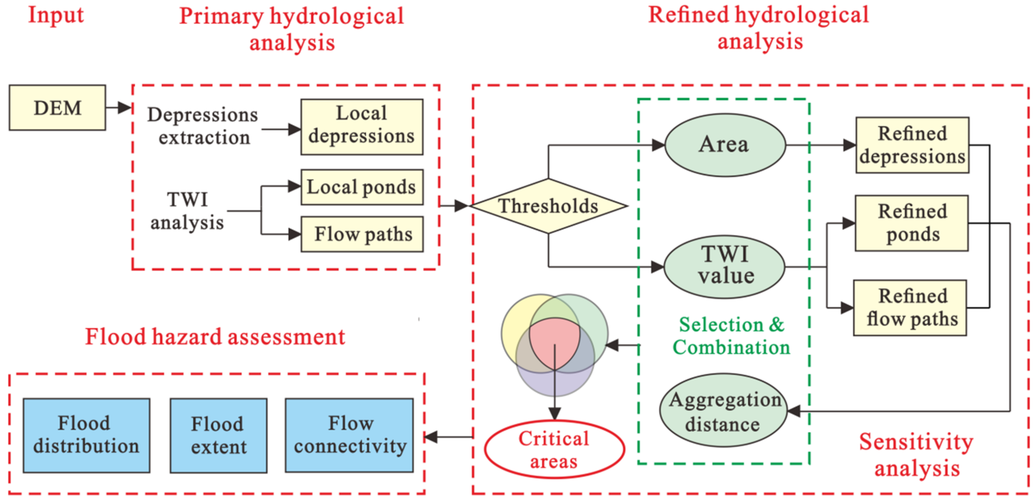
Figure 1 shows the flow chart of the GIS-based hydrological modeling approach with inputs of the regional Digital Elevation Model (DEM). Two stages of analysis were adopted to identify flood-prone areas, including information on their distributions, extents and flow paths. The primary hydrological analysis included depression extraction (DE) and topographic wetness index (TWI) [35,36] assessments. Specifically, the depressions were regarded as the basic inundated area in the terrain [33,34]. The TWI combined the information of the upstream contributing area and slope to estimate the surface flow directions and spatial distributions of the accumulated flows with a description of the topographic data [37]. The local depressions are characterized using the Fill and Cutfill functions, and the TWI analysis captures the local ponds and flow paths concurrently by adopting an integration of the GIS functions of the flow direction, flow accumulation, slope and raster calculator.
The refined hydrological analysis aims to take full advantage of the DE and TWI analyses and optimize the identification of flood depressions and flow paths by strategically aggregating their outputs with proper threshold selection/criterion. Three types of thresholds were adopted—namely, the depression area of DE, TWI value and the aggregation distance for the spatial capturing and aggregation of refined ponds and flow paths. The total number of combinations can be assessed given the number of thresholds considered (i.e., TA, TTWI and TAD refer to the numbers of thresholds used for areas, TWI values and aggregation distances, respectively). That means, in total, there are TA × TTWI × TAD kinds of combination options to be considered. The next step is to compare each option with a baseline model/flood map to assess the performance of the refined hydrological analysis. We then identified the threshold combinations that can best characterize the flood-prone areas. In doing so, it provides guidance on the proper threshold criterion for similar types of studies and, thus, can save a large amount of time by eliminating the work on estimating the refined hydrological analysis for the full set of combination options.
2.2. Performance Indicators
There are two types of performance evaluations. The first one is the visual comparison that shows the flow paths and local depressions captured spatially by different scenarios in comparison to the outputs from the baseline model. More importantly, the second measure is the quantitative assessments of the model performance. A binary coding method was applied to the raster of the GIS flooding maps by labeling the flooded and dry raster cells with a value of 1 and 0, respectively. On the basis of that, two types of indicators that are commonly acknowledged and used in the literature—namely, F1 and F2, shown in Equations (1) and (2)—were adopted in this study. The F1 indicator is reported to be a relatively unbiased measure that equitably discriminates between underpredictions and overprediction. (i.e., misses and false alarms) [34,38,39,40,41,42,43]. However, as the penalization for overprediction is quite weak, it is likely to result in overestimated outputs. The F2 indicator was proposed to penalize the tendency of overprediction [38,40,42]; nevertheless, the intensity of penalization seems heavy and can easily lead to underestimated predictions and, thus, needs to be further discussed and altered.
In this study, to better moderate the penalization of the over- and underpredictions formulated in the aforementioned two types of indicators, a new performance indicator F3 is proposed; see Equation (3). Note that we lightened the penalization intensity in this indicator in comparison to the F2. The physical reason for the F3 indicator is that displacements occur, and they are penalized significantly in the standard formulation.
where Hits are the number of cells that are both flooded in our model and the baseline model (see the explanations in Table 1) [38,39,40]; False alarms are outputs that are flooded in our model but dry in the baseline model and vice versa. Misses are outputs that are dry in our model but flooded in the baseline model; Correct Negatives refers to the number of cells that floods are both absent in the two models. Noted that the higher the quality of the model, the more hits and correct negatives, and simultaneously, less false alarms and misses [39]. In addition, high values of the false alarms and misses represent the possible tendencies of overprediction and underprediction in the tested model [38,39].
F1 = Hits/(Hits + False alarms + Misses)
F2 = (Hits − False alarms))/(Hits + False alarms + Misses)
F3 = (Hits − (False alarms)/2)/(Hits + False alarms + Misses)
2.3. Case Study
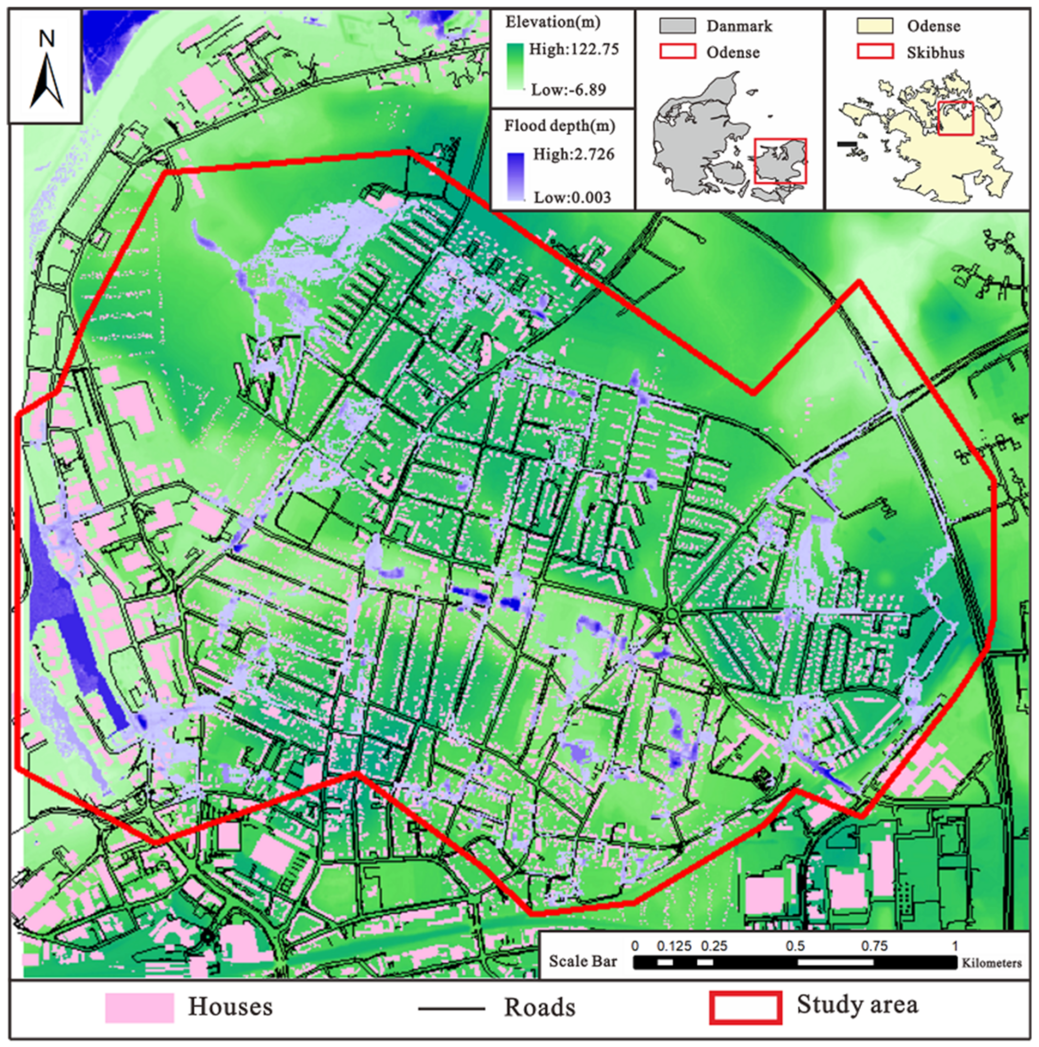
The city of Skibhus located in the north center of Odense, Denmark was adopted for the case study (see Figure 2). The area is 389 ha, and the main land use is residential, with a transportation network and a small amount of commercial and industrial activities. The coordination system of Denmark is WGS 1984 UTM ZONE 32N. The regional Digital Elevation Model (DEM) was obtained based on LIDAR technology and has a resolution of 5.0 × 5.0 m. The elevation ranges from −6.89 to 122.75 m. The baseline model is a combined 1D/2D model simulated using Mike Urban and Mike Flood [44]. The 1D sewer system is a combined drainage that conveys water from east to west towards the outlets near Odense Harbor. The key model parameters, such as surface imperviousness and time of concentration, were calibrated to obtain reasonable model simulations of flows in several key manholes in the sewer system against observed rainfall events. The model quality is reasonably good and has been used for multiple studies in flood analyses and risk management [44,45]. As a result, the baseline scenario describes the distributions and extents of flood-prone areas under extreme precipitation events. It is shown that a larger extent of the flood-prone area lies in the center and northwest part of the area, and most of the rest spreads along the road network. Certainly, it is noted that, despite the high-resolution mapping by the 1D/2D model, uncertainties are inherently associated with the baseline scenario.
3. Results and Discussion
3.1. Depressions Extraction (DE) Analysis
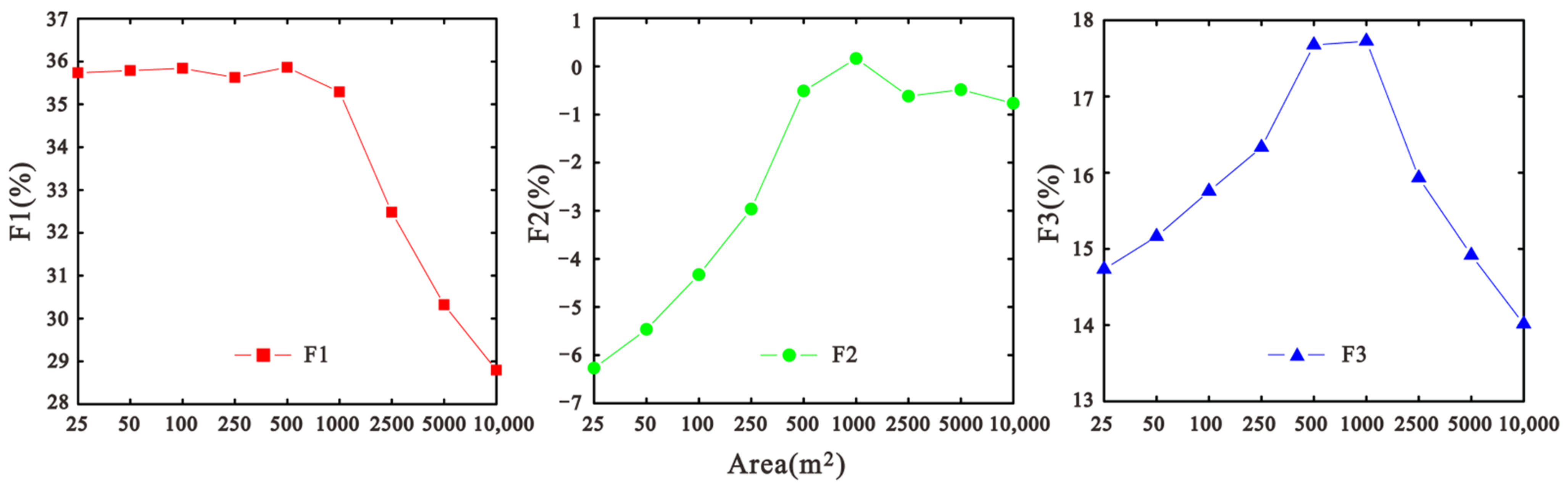
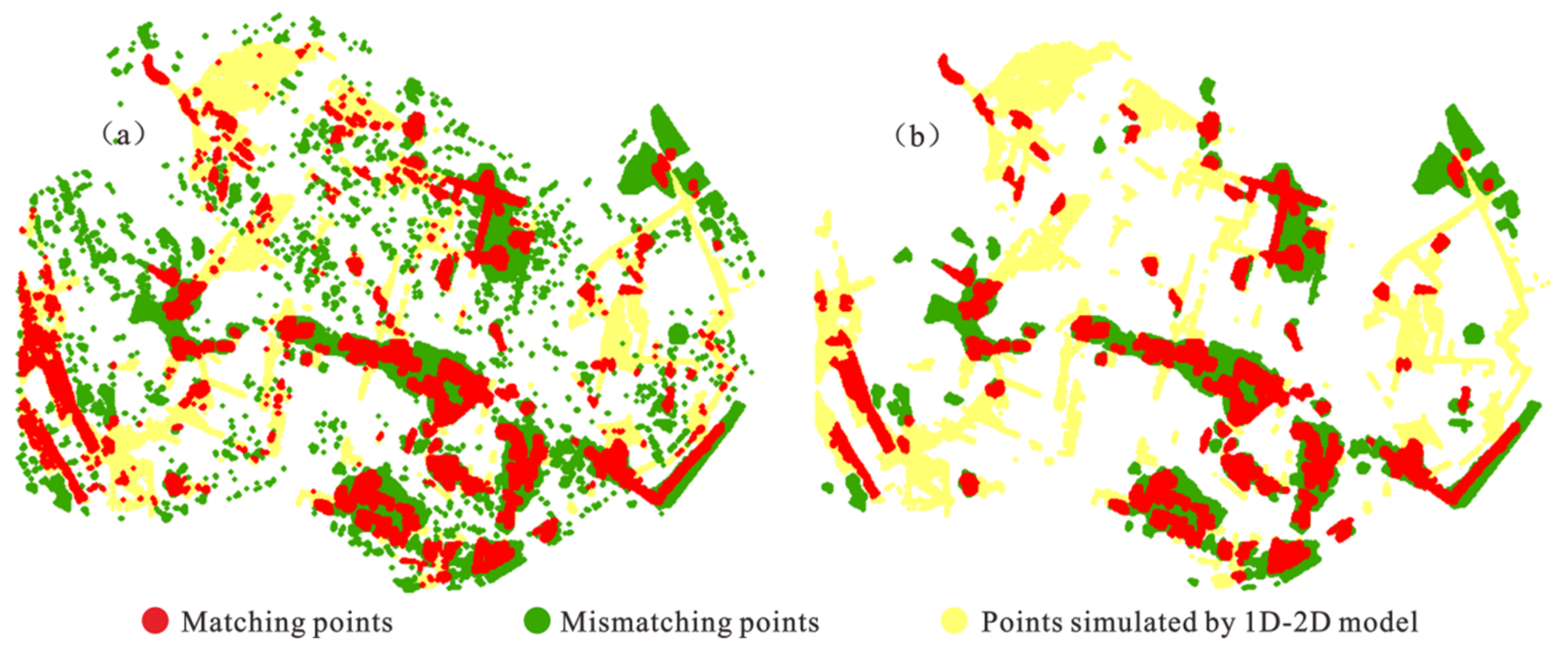
Figure 3 shows the calculated three types of indicators as a function of the extraction area (i.e., the size of the depressions) for the DE method. A general tendency is that all the three curves rise at first and then decline with the increasing extraction area. Note that all peaks fall around the median thresholds (i.e., between 500 and 1000 m2) despite the achieved values that differ for the three types of indicators. This indicates that, for local depression identification, mid-values of the thresholds (i.e., extraction area) are generally suggested to achieve a refined DE analysis. Figure 4 shows the difference between the flood maps by the conventional and refined DE methods, respectively. As the conventional DE often uses the lower bound of the threshold (i.e., a small extraction area) and, thus, all sizes of depressions are captured, which can easily result in a large number of invalid locations of flood-prone areas (Figure 4a). In contrast, the refined DE with the mid-value of the threshold manages to find larger depressions with actual impacts on the floods, and thus, the flood-prone area mapping is improved. Nevertheless, it is noteworthy that the ability of the DE analysis in capturing the local flow paths (e.g., runoffs on the road network and open channels) is weak (Figure 4b).
3.2. TWI Analysis
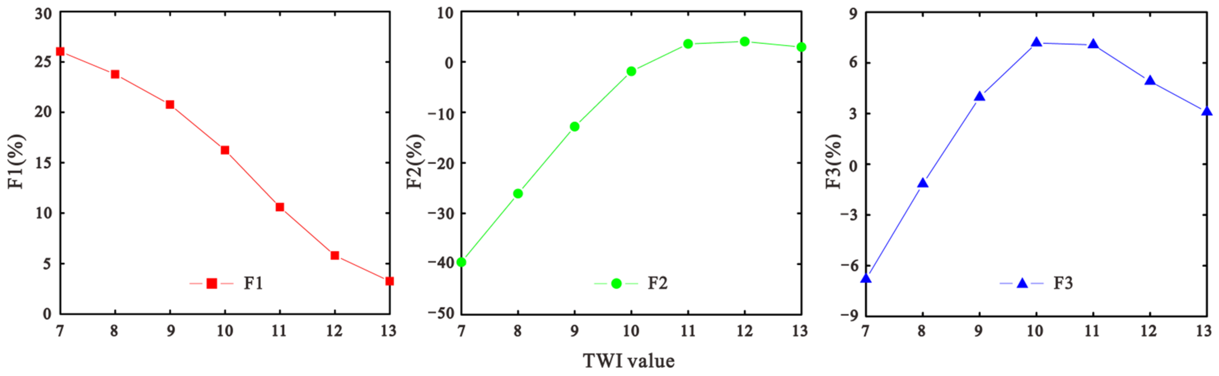
Figure 5 shows that distinct results were obtained for the three types of indicators as a function of the calculated TWI values. The F1 indicator continued to decline with the increase in the TWI threshold. As a result, the minimum value of the threshold leads to the best model performance. As for F2, it first increases swiftly and then decreases along with the increasing threshold. The best output is obtained near the end of the curve (i.e., at the value of 12). A similar tendency is shown in the F3 curve, whereas the peak value occurs around the mid-value of the threshold (i.e., at the value of 10).
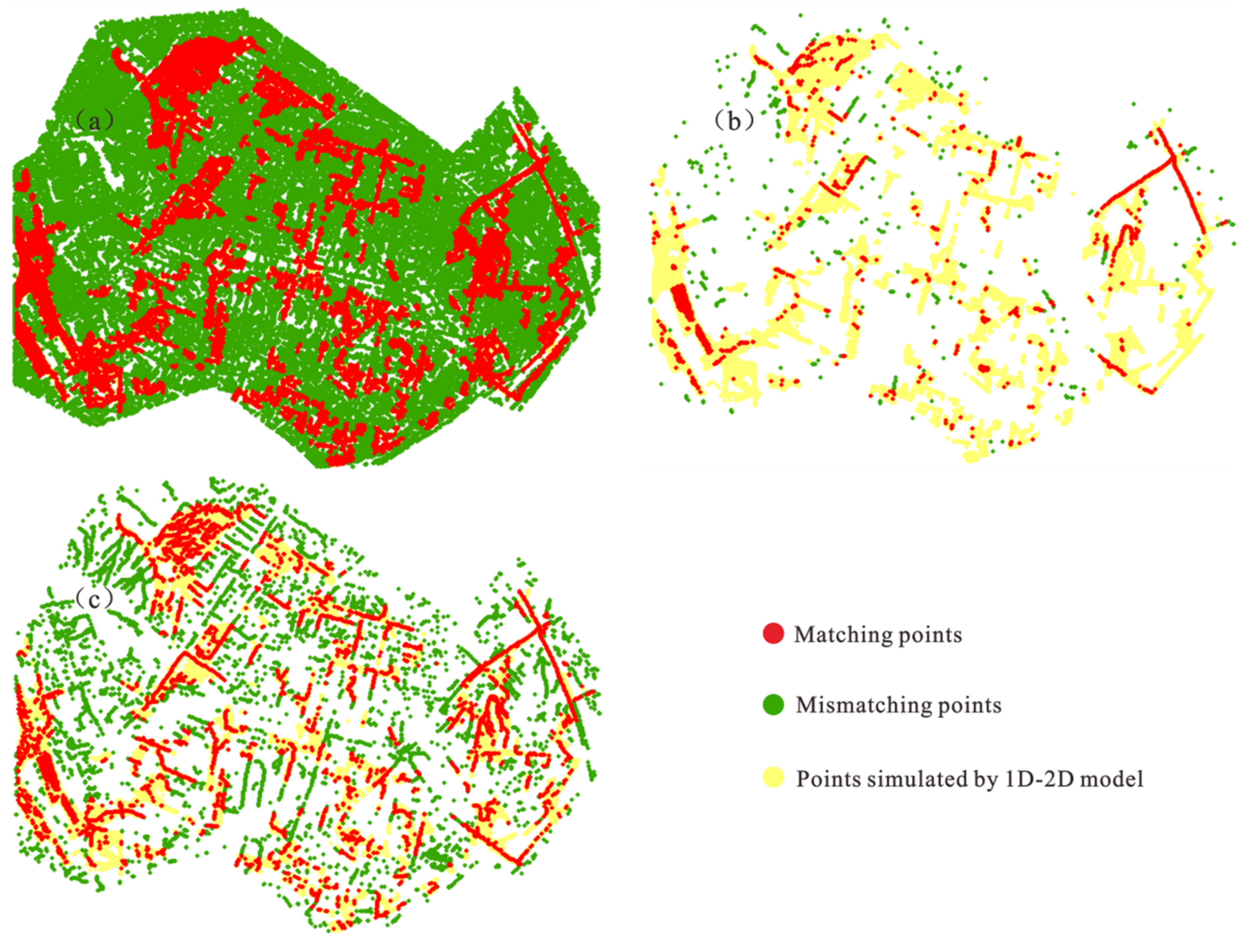
In terms of visual quality, the spatial illustrations of the optimal results achieved based on the three types of indicators are shown in Figure 6. It is seen that the flood extent is seriously overestimated, using the F1 indicator, and a large amount of useless information is present. The mismatching points cover almost the entire region, and it is almost impossible to identify the actual flood-prone areas (Figure 6a). On the contrary, there is too little information to support the flood characterization based on the F2 indicator (Figure 6b). This clearly illustrates the constraints of the first two types of indicators. F1 proposes too-light penalization for overprediction, whereas F2 is too heavy. As for F3, more effective information for flood mapping is captured (Figure 6c). Nevertheless, the refined TWI method still showed a trend of overestimation of the flood ponds and flow paths and a failure of characterizing large inundation areas.
3.3. Aggregation of DE and TWI Outputs
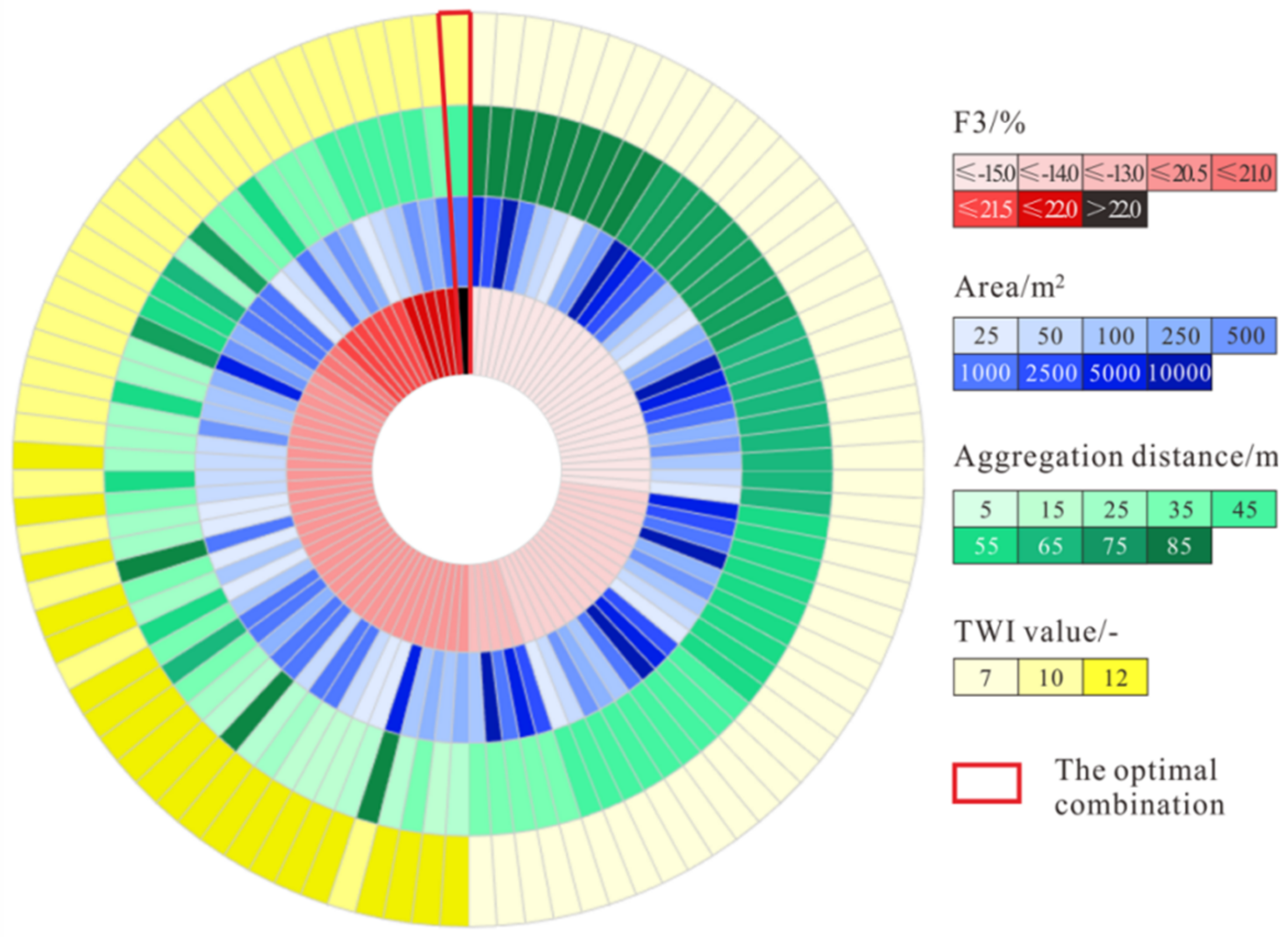
As F3 showed a higher adaptability in evaluating the DE and TWI methods, it was adopted as the performance indicator in the aggregation analysis. We sorted all the combination options (i.e., 567 options) according to the calculated F3 values and selected 100 options (i.e., top 50 and bottom 50 ones) as representative samples to illustrate the impacts of the three types of thresholds on the hazard mapping performance (see Figure 7). To be specific, the innermost circle of the compass plot shows the obtained F3 value for the specific threshold options. The outer three circles describe the corresponding thresholds (i.e., DE area, TWI value and aggregation distance between the extracted DE and TWI features) used to characterize the flood-prone areas, respectively. The optimal option is highlighted by the red fan.
It is found that the optimal option is achieved by adopting the mid-values of all the thresholds. This information is important to further guide a refined hydrological analysis as the practitioners do not need to repeat the full set of the combination options but are suggested to use the optimal thresholds directly for flood-prone area mapping. By doing so, it can significantly reduce the computation time and improve the modeling efficiency, which is especially essential for rapid flood mapping. Further, it is noted that the impacts of the DE area on the flood mapping performance are less significant in comparison to the TWI values and aggregation distance. For the top five options, the adopted TWI value is constant (i.e., the median value, TWI = 10). The aggregation distances vary between 35 and 45 m, which are also located near the middle position of the threshold boundaries. The values of the extraction area differ to a larger extent; however, they mainly contain smaller values of the thresholds. The results indicate that the TWI threshold is most important because that is the most consistent indicator when selecting the best options. Given its great impacts on flood mapping, priority should be given to the TWI threshold selections in order to improve their ability in hydrological characterization.
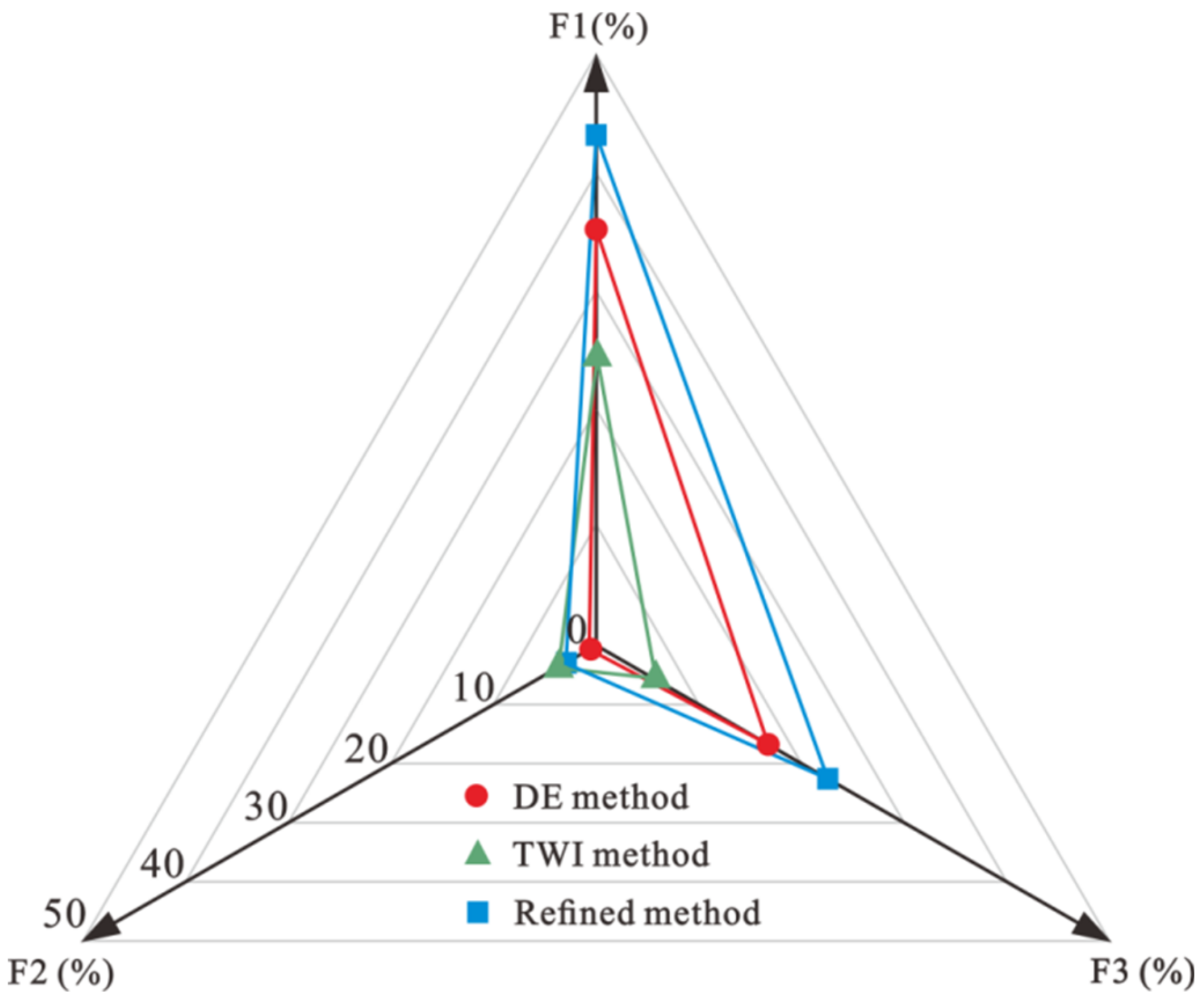
Figure 8 shows that the refined hydrological approach outperforms the DE and TWI methods according to all three indicators. Specifically, F1 and F2 increased by 8% (i.e., from 36% to 44%) and 3% (from 0.16% to 3%) by adopting the refined method instead of the DE method, respectively. As for F3, the values obtained are 18%, 7% and 23% using the DE, TWI and refined methods, respectively. The spatial illustrations of the three types of methods with their optimal thresholds are shown in Figure 9. It is clear that the DE and TWI methods have the constraints of capturing too little and too much information. The DE method mainly identifies the flood-prone areas located in large low depressions; however, it fails to capture the floods along the flow pathways (e.g., transportation network). In contrast, the TWI method mainly extracts small-scale flood-prone areas and, thus, presents many invalid locations for flood mapping. The refine method with optimized thresholds manages to take full advantage of both methods and achieves a more effective flood mapping performance.
3.4. Testing Case Study
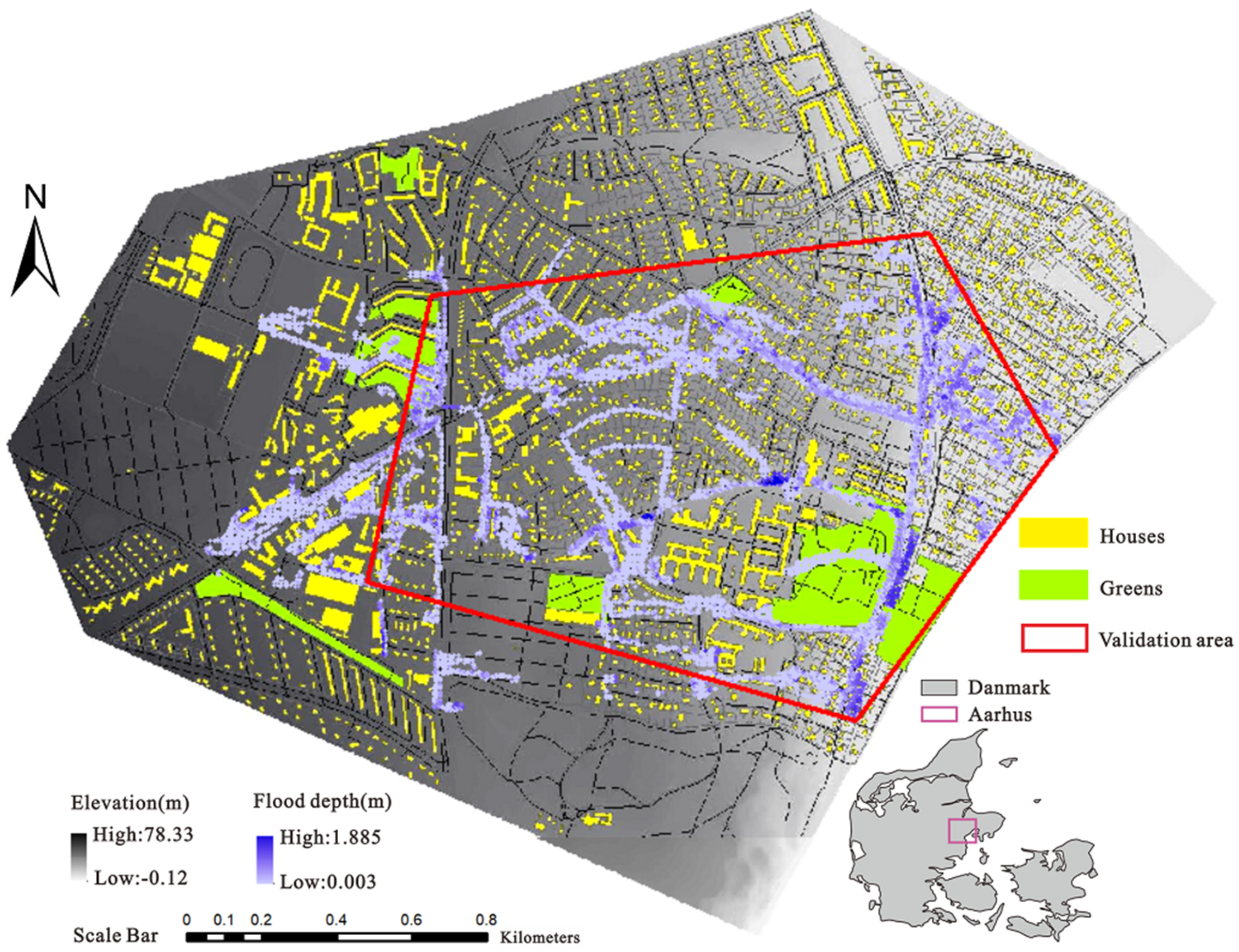
The testing case is located in the catchment of Risskov, in the northern part of Aarhus City, Denmark (see Figure 10). The catchment size is about 377 ha, and the main land use is also residential. Commercial and industrial activities are marginal in the case area. The topography is high in the west and low in the east, with regional elevation ranges between −0.12 and 78 m. The local drainage system is a separate system that conveys the water from the west to the outlets along the coastline. The flood map used as the validation scenario is simulated using a 1D/2D-coupled model established in Mike Urban and Mike Flood [46,47]. The model is validated with descriptions of catchment imperviousness and historical inundation zones.
The results obtained in the validation case are consistent with the ones from the Odense case. The optimal flood mapping is achieved using the medians of the three types of thresholds (i.e., DE area of 150 m2, TWI of 9 and aggregation distance of 45 m). The F3 indicator is estimated to be 9.27%, 11.83% and 25.63% using the three types of mapping methods, respectively. That is to say, F3 increases by 16% and 14% thanks to the refined approach in comparison to the DE and TWI methods. Meanwhile, the spatial illustrations of the three methods are compared in Figure 11. Similarly, our approach is capable of characterizing more flow paths and depressions with actual influences on floods compared to the traditional DE and TWI methods. The flood mapping is more accurate and efficient, and thus, the methodology proposed is feasible and maintains good applicability in identifying flood-prone zones in other case studies.
4. Conclusions
Facing increasing flood damages, improving technologies on rapid and yet robust hazard mapping helps to provide decision-makers with better support to predict, analyze and manage the impacts of urban flooding. At present, urban flood modeling is developing towards the direction of refinement and efficiency. How to quickly and accurately characterize flood-prone areas in the context of large-scale emergency assessment and data limitation is one of the key problems to be solved. This study explored a refined hydrological characterization methodology of flood-prone areas by taking advantage of the traditional depression extraction and TWI analyses. Strategic characterization and combination rules were proposed to provide a prompt but relatively accurate flood mapping with limited data input. Equally important, a new performance indicator (i.e., F3) was introduced in this study to improve the hazard mapping assessment.
The results show that the mid-values of the three types of thresholds (i.e., extraction area, TWI value and aggregation distance) are suggested to be adopted to achieve the optimal performance for the individual and combined methods. The constraints of the DE and TWI methods are clearly seen in the spatial mapping of the assessed flood-prone areas, where DE and TWI captured too little or too many details. The refined method takes advantage of both methods and outperforms them according to all the three types of performance indicators. Equally important, the refined method has a much lower demand on the data and computation efforts in comparison to the calculations using a full set of combination options and the sophisticated 1D/2D-coupled modeling technology.
Some limitations of this study should be acknowledged. This method is suitable for large-scale and emergency assessments (i.e., distribution and extent of flood hazards) due to the deficient information and inadequate descriptions on flood depths. In addition, the method is dependent on the raster accuracy of DEM and digital map, and further analyses of open-source data are needed to ensure the accuracy of the analysis. In the future work, correction methods of key topographic parameters and the underlying mechanisms of microtopographic influences (e.g., complex underlying surfaces, special terrain and building conditions) on hazard characterization can be explored to achieve a more accurate mapping of flood-prone areas. Despite the limitations, this methodology provides decision-makers a rapid and effective analysis tool on flood hazard mapping for formulating a defense, mitigation, and management measures aiming to reduce the damages under the challenges of urbanization and climate change.
Author Contributions
Conceptualization, Q.Z. and J.S.; methodology, Q.Z., J.S. and K.A.-N.; software, J.S. validation, J.L., Z.Y. and J.F.; formal analysis, investigation, Q.Z. and J.S.; writing—original draft preparation, Q.Z. and J.S.; writing—review and editing, K.A.-N. and Y.R.; project administration, Q.Z.; funding acquisition, Q.Z. All authors have read and agreed to the published version of the manuscript.
Funding
This research was funded by the National Natural Science Foundation of China (Grant No. 51809049), the Science and Technology Program of Guangzhou, China (Grant No. 201804010406).
Institutional Review Board Statement
Not applicable.
Informed Consent Statement
Not applicable.
Acknowledgments
The Water Center South, Denmark and Aarhus Water, Denmark are gratefully acknowledged for supplying the catchment data used in this study.
Conflicts of Interest
The authors declare they have no conflicts of interest.
References
- Wang, Z.; Wang, H.; Huang, J.; Kang, J.; Han, D. Analysis of the Public Flood Risk Perception in a Flood-Prone City: The Case of Jingdezhen City in China. Water 2018, 10, 1577. [Google Scholar] [CrossRef] [Green Version]
- Yin, J.; Yu, D.; Yin, Z.; Liu, M.; He, Q. Evaluating the impact and risk of pluvial flash flood on intra-urban road network: A case study in the city center of Shanghai, China. J. Hydrol. 2016, 537, 138–145. [Google Scholar] [CrossRef] [Green Version]
- Field, C.B.; Barros, V.R.; Dokken, D.J.; Mach, K.J.; Mastrandrea, M.D.; Bilir, T.E.; Chatterjee, M.; Ebi, K.L.; Estrada, Y.O.; Genova, R.C.; et al. AR5 Climate Change 2014: Impacts, Adaptation, and Vulnerability, Global and Sectoral Aspects, Working Group II Contribution to the Fifth Assessment Report of the Intergovernmental Panel on Climate Change; Cambridge University Press: New York, NY, USA, 2014; pp. 35–94. [Google Scholar]
- Simonovic, S.P. Bringing Future Climatic Change into Water Resources Management Practice Today. Water Resour. Manag. 2017, 31, 2933–2950. [Google Scholar] [CrossRef]
- Zhou, Q.; Leng, G.; Su, J.; Ren, Y. Comparison of urbanization and climate change impacts on urban flood volumes: Importance of urban planning and drainage adaptation. Sci. Total. Environ. 2019, 658, 24–33. [Google Scholar] [CrossRef] [PubMed]
- Huong, H.T.L.; Pathirana, A. Urbanization and climate change impacts on future urban flooding in Can Tho City, Vietnam. Hydrol. Earth Syst. Sci. 2013, 17, 379–394. [Google Scholar] [CrossRef] [Green Version]
- Zhang, N.; Luo, Y.J.; Chen, X.Y.; Li, Q.; Jing, Y.C.; Wang, X.; Feng, C.H. Understanding the effects of composition and configuration of land covers on surface runoff in a highly urbanized area. Ecol. Eng. 2018, 125, 11–25. [Google Scholar] [CrossRef]
- Alfieri, L.; Feyen, L.; Di Baldassarre, G. Increasing flood risk under climate change: A pan-European assessment of the benefits of four adaptation strategies. Clim. Chang. 2016, 136, 507–521. [Google Scholar] [CrossRef] [Green Version]
- Mahmoud, S.H.; Gan, T.Y. Urbanization and climate change implications in flood risk management: Developing an efficient decision support system for flood susceptibility mapping. Sci. Total Environ. 2018, 636, 152–167. [Google Scholar] [CrossRef]
- Kundzewicz, Z.W.; Su, B.D.; Wang, Y.J.; Wang, G.J.; Wang, G.F.; Huang, J.L.; Jiang, T. Flood risk in a range of spatial perspectives—From global to local scales. Nat. Hazards Earth Syst. Sci. 2019, 19, 1319–1328. [Google Scholar] [CrossRef] [Green Version]
- Zhou, Q.Q.; Leng, G.Y.; Feng, L.Y. Predictability of state-level flood damage in the conterminous United States: The role of hazard, exposure and vulnerability. Sci. Rep. 2017, 7, 11. [Google Scholar] [CrossRef] [Green Version]
- Zhou, Q.Q.; Su, J.H.; Leng, G.Y.; Peng, J. The role of hazard and vulnerability in modulating economic damages of inland floods in the United States using a survey-based dataset. Sustainability 2019, 11, 3754. [Google Scholar] [CrossRef] [Green Version]
- Dottori, F.; Kalas, M.; Salamon, P.; Bianchi, A.; Alfieri, L.; Feyen, L. An operational procedure for rapid flood risk assessment in Europe. Nat. Hazards Earth Syst. Sci. 2017, 17, 1111–1126. [Google Scholar] [CrossRef] [Green Version]
- Gain, A.K.; Hoque, M.M. Flood risk assessment and its application in the eastern part of Dhaka City, Bangladesh. J. Flood Risk Manag. 2013, 6, 219–228. [Google Scholar] [CrossRef]
- Vu, T.T.; Ranzi, R. Flood risk assessment and coping capacity of floods in central Vietnam. J. Hydro-Environ. Res. 2017, 14, 44–60. [Google Scholar] [CrossRef]
- Yang, C.R.; Tsai, C.T. Development of a gis-based flood information system for floodplain modeling and damage calculation. J. Am. Water Resour. Assoc. 2000, 36, 567–577. [Google Scholar] [CrossRef]
- Dang, A.T.N.; Kumar, L. Application of remote sensing and GIS-based hydrological modelling for flood risk analysis: A case study of District 8, Ho Chi Minh City, Vietnam. Geomat. Nat. Hazards Risk 2017, 8, 1792–1811. [Google Scholar] [CrossRef] [Green Version]
- Alho, P.; Aaltonen, J. Comparing a 1d hydraulic model with a 2d hydraulic model for the simulation of extreme glacial outburst floods. Hydrol. Process. 2008, 22, 1537–1547. [Google Scholar] [CrossRef]
- Jung, Y.; Merwade, V.; Yeo, K.; Shin, Y.; Lee, S.O. An approach using a 1d hydraulic model, landsat imaging and generalized likelihood uncertainty estimation for an approximation of flood discharge. Water 2013, 5, 1598–1621. [Google Scholar] [CrossRef] [Green Version]
- Djordjevic, S.; Prodanovic, D.; Walters, G.A. Simulation of transcritical flow in pipe/channel networks. J. Hydraul. Eng. 2004, 130, 1167–1178. [Google Scholar] [CrossRef]
- Bulti, D.T.; Abebe, B.G. A review of flood modeling methods for urban pluvial flood application. Model. Earth Syst. Environ. 2020, 6, 1293–1302. [Google Scholar] [CrossRef]
- Yu, H.J.; Huang, G.R. A coupled 1d and 2d hydrodynamic model for free-surface flows. Proc. Inst. Civil. Eng. Water Manag. 2014, 167, 523–531. [Google Scholar] [CrossRef]
- Patel, D.P.; Ramirez, J.A.; Srivastava, P.K.; Bray, M.; Han, D.W. Assessment of flood inundation mapping of Surat city by coupled 1d/2d hydrodynamic modeling: A case application of the new hec-ras 5. Nat. Hazards 2017, 89, 93–130. [Google Scholar] [CrossRef]
- Van Dijk, E.; van der Meulen, J.; Kluck, J.; Straatman, J.H.M. Comparing modelling techniques for analysing urban pluvial flooding. Water Sci. Technol. 2014, 69, 305–311. [Google Scholar] [CrossRef] [PubMed]
- Bisht, D.S.; Chatterjee, C.; Kalakoti, S.; Upadhyay, P.; Sahoo, M.; Panda, A. Modeling urban floods and drainage using swmm and mike urban: A case study. Nat. Hazards 2016, 84, 749–776. [Google Scholar] [CrossRef]
- Vozinaki, A.E.K.; Morianou, G.G.; Alexakis, D.D.; Tsanis, I.K. Comparing 1d and combined 1d/2d hydraulic simulations using high-resolution topographic data: A case study of the Koiliaris basin, Greece. Hydrol. Sci. J. 2017, 62, 642–656. [Google Scholar] [CrossRef]
- Vojinovic, Z.; Tutulic, D. On the use of 1d and coupled 1d-2d modelling approaches for assessment of flood damage in urban areas. Urban Water J. 2009, 6, 183–199. [Google Scholar] [CrossRef]
- Leandro, J.; Chen, A.S.; Djordjevic, S.; Savic, D.A. Comparison of 1d/1d and 1d/2d coupled (sewer/surface) hydraulic models for urban flood simulation. J. Hydraul. Eng. 2009, 135, 495–504. [Google Scholar] [CrossRef]
- Leandro, J.; Djordjevic, S.; Chen, A.S.; Savic, D.A.; Stanic, M. Calibration of a 1d/1d urban flood model using 1d/2d model results in the absence of field data. Water Sci. Technol. 2011, 64, 1016–1024. [Google Scholar] [CrossRef] [Green Version]
- Yu, D.P.; Yin, J.; Liu, M. Validating city-scale surface water flood modelling using crowd-sourced data. Environ. Res. Lett. 2016, 11, 21. [Google Scholar] [CrossRef]
- Chen, A.S.; Evans, B.; Djordjević, S.; Savić, D.A. Multi-layered coarse grid modelling in 2d urban flood simulations. J. Hydrol. 2012, 470–471, 1–11. [Google Scholar] [CrossRef] [Green Version]
- Ghimire, B.; Chen, A.S.; Guidolin, M.; Keedwell, E.C.; Djordjević, S.; Savić, D.A. Formulation of a fast 2d urban pluvial flood model using a cellular automata approach. J. Hydroinform. 2013, 15, 676–686. [Google Scholar] [CrossRef] [Green Version]
- Zhang, S.H.; Pan, B.Z. An urban storm-inundation simulation method based on gis. J. Hydrol. 2014, 517, 260–268. [Google Scholar] [CrossRef]
- Jamali, B.; Lowe, R.; Bach, P.M.; Urich, C.; Arnbjerg-Nielsen, K.A.; Deletic, A. A rapid urban flood inundation and damage assessment model. J. Hydrol. 2018, 564, 1085–1098. [Google Scholar] [CrossRef]
- Beven, K.J.; Kirkby, M.J. A physically based, variable contributing area model of basin hydrology. Hydrol. Sci. J. 1979, 24, 43–69. [Google Scholar] [CrossRef] [Green Version]
- Sorensen, R.; Zinko, U.; Seibert, J. On the calculation of the topographic wetness index: Evaluation of different methods based on field observations. Hydrol. Earth Syst. Sci. 2006, 10, 101–112. [Google Scholar] [CrossRef] [Green Version]
- Zhou, Q.Q.; Blohm, A.; Liu, B. Planning framework for mesolevel optimization of urban runoff control schemes. J. Water Resour. Plan. Manag. ASCE 2017, 143, 04016083. [Google Scholar] [CrossRef]
- Schumann, G.; Bates, P.D.; Horritt, M.S.; Matgen, P.; Pappenberger, F. Progress in integration of remote sensing–derived flood extent and stage data and hydraulic models. Rev. Geophys. 2009, 47, 47. [Google Scholar] [CrossRef]
- Bennett, N.D.; Croke, B.F.; Guariso, G.; Guillaume, J.H.; Hamilton, S.; Jakeman, A.J.; Marsili-Libelli, S.; Newham, L.T.; Norton, J.P.; Perrin, C.; et al. Characterising performance of environmental models. Environ. Model. Softw. 2013, 40, 1–20. [Google Scholar] [CrossRef]
- Pappenberger, F.; Frodsham, K.; Beven, K.; Romanowicz, R.; Matgen, P. Fuzzy set approach to calibrating distributed flood inundation models using remote sensing observations. Hydrol. Earth Syst. Sci. 2007, 11, 739–752. [Google Scholar] [CrossRef] [Green Version]
- Lhomme, J.; Sayers, P.; Gouldby, B.; Samuels, P.; Wills, M.; Mulet-Marti, J. Recent development and application of a rapid flood spreading method. In Flood Risk Management: Research and Practice; Taylor & Francis Group: London, UK, 2008; pp. 15–24. [Google Scholar]
- Hunter, N.M.; Bates, P.D.; Horritt, M.S.; Roo, P.J.D.; Werner, M.G.F. Utility of different data types for calibrating flood inundation models within a glue framework. Hydrol. Earth Syst. Sci. 2005, 9, 412–430. [Google Scholar] [CrossRef]
- Davidsen, S.; Löwe, R.; Thrysøe, C.; Arnbjerg-Nielsen, K. Simplification of one-dimensional hydraulic networks by automated processes evaluated on 1d/2d deterministic flood models. J. Hydroinform. 2017, 19, 686–700. [Google Scholar] [CrossRef] [Green Version]
- Zhou, Q.; Mikkelsen, P.S.; Halsnaes, K.; Arnbjerg-Nielsen, K. Framework for economic pluvial flood risk assessment considering climate change effects and adaptation benefits. J. Hydrol. 2012, 414, 539–549. [Google Scholar] [CrossRef]
- Zhou, Q.; Halsnæs, K.; Arnbjerg-Nielsen, K. Economic assessment of climate adaptation options for urban drainage design in Odense, Denmark. Water Sci. Technol. 2012, 66, 1812–1820. [Google Scholar] [CrossRef] [PubMed] [Green Version]
- Zhou, Q.; Panduro, T.; Thorsen, B.; Arnbjerg-Nielsen, K. Adaption to extreme rainfall with open urban drainage system: An integrated hydrological cost-benefit analysis. Environ. Manag. 2013, 51, 586–601. [Google Scholar] [CrossRef] [Green Version]
- Zhou, Q.; Panduro, T.E.; Thorsen, B.J.; Arnbjerg-Nielsen, K. Verification of flood damage modelling using insurance data. Water Sci. Technol. 2013, 67, 1362–1369. [Google Scholar] [CrossRef]
Figure 1.
Workflow of the GIS-based characterization of the flood-prone areas.

Figure 2.
Descriptions of the urban land use, topography and flood-prone areas of the study area.

Figure 3.
The three types of indicators: F1, F2 and F3, as a function of the extraction area.

Figure 4.
Comparison of the flood-prone areas captured by (a) conventional and (b) refined DE analyses, respectively. Three types of points are all shown on the 5.0 × 5.0-m resolution and include the matching, mismatching and the flooded points simulated by the baseline model.
Figure 4.
Comparison of the flood-prone areas captured by (a) conventional and (b) refined DE analyses, respectively. Three types of points are all shown on the 5.0 × 5.0-m resolution and include the matching, mismatching and the flooded points simulated by the baseline model.

Figure 5.
The three types of indicators: F1, F2 and F3 as a function of the TWI value.

Figure 6.
Spatial illustrations of flood maps using optimized TWI thresholds based on the (a) F1, (b) F2 and (c) F3 indicators. All points are shown on the 5.0 × 5.0-m resolution.
Figure 6.
Spatial illustrations of flood maps using optimized TWI thresholds based on the (a) F1, (b) F2 and (c) F3 indicators. All points are shown on the 5.0 × 5.0-m resolution.

Figure 7.
Selected representative options (i.e., top 50 and bottom 50 ranked according to the F3 values) out of the full set of combinations (i.e., 567 options).
Figure 7.
Selected representative options (i.e., top 50 and bottom 50 ranked according to the F3 values) out of the full set of combinations (i.e., 567 options).

Figure 8.
The three types of indicators: F1, F2 and F3 achieved by the DE, TWI and refined methods based on their optimal thresholds, respectively.
Figure 8.
The three types of indicators: F1, F2 and F3 achieved by the DE, TWI and refined methods based on their optimal thresholds, respectively.

Figure 9.
Spatial illustrations of the flood maps using optimized (a) DE, (b) TWI and (c) refined methods based on the F3 indicator.
Figure 9.
Spatial illustrations of the flood maps using optimized (a) DE, (b) TWI and (c) refined methods based on the F3 indicator.

Figure 10.
Descriptions of the land use, topography and flood map used as the validation scenario.

Figure 11.
Spatial illustrations of flood maps using optimized (a) DE, (b) TWI and (c) refined methods based on the F3 indicator in the validation area.
Figure 11.
Spatial illustrations of flood maps using optimized (a) DE, (b) TWI and (c) refined methods based on the F3 indicator in the validation area.


Table 1.
Descriptions of the four types of parameters in the model performance evaluations.
| Baseline Model | |||
|---|---|---|---|
| Flooded/Wet | Dry | ||
| Tested model | Flooded/wet | Hits | False alarms |
| Dry | Misses | Correct Negatives | |
Publisher’s Note: MDPI stays neutral with regard to jurisdictional claims in published maps and institutional affiliations. |
© 2021 by the authors. Licensee MDPI, Basel, Switzerland. This article is an open access article distributed under the terms and conditions of the Creative Commons Attribution (CC BY) license (https://creativecommons.org/licenses/by/4.0/).
Share and Cite
MDPI and ACS Style
Zhou, Q.; Su, J.; Arnbjerg-Nielsen, K.; Ren, Y.; Luo, J.; Ye, Z.; Feng, J. A GIS-Based Hydrological Modeling Approach for Rapid Urban Flood Hazard Assessment. Water 2021, 13, 1483. https://doi.org/10.3390/w13111483
AMA Style
Zhou Q, Su J, Arnbjerg-Nielsen K, Ren Y, Luo J, Ye Z, Feng J. A GIS-Based Hydrological Modeling Approach for Rapid Urban Flood Hazard Assessment. Water. 2021; 13(11):1483. https://doi.org/10.3390/w13111483
Chicago/Turabian StyleZhou, Qianqian, Jiongheng Su, Karsten Arnbjerg-Nielsen, Yi Ren, Jinhua Luo, Zijian Ye, and Junman Feng. 2021. "A GIS-Based Hydrological Modeling Approach for Rapid Urban Flood Hazard Assessment" Water 13, no. 11: 1483. https://doi.org/10.3390/w13111483
Note that from the first issue of 2016, this journal uses article numbers instead of page numbers. See further details here.