Nonlinear Shear Effects of the Secondary Current in the 2D Flow Analysis in Meandering Channels with Sharp Curvature

1
Korea Institute of Civil Engineering and Building Technology, Goyangdae-Ro, Ilsanseo-Gu, Goyang-Si 10223, Korea
2
Department of Civil Engineering, Seoul National University, 1 Gwanak-Ro, Gwanak-Gu, Seoul 08826, Korea
*
Author to whom correspondence should be addressed.
Water 2021, 13(11), 1486; https://doi.org/10.3390/w13111486
Submission received: 30 April 2021
/
Revised: 22 May 2021
/
Accepted: 23 May 2021
/
Published: 26 May 2021
(This article belongs to the Section Hydraulics and Hydrodynamics)
Abstract
:In order to analyze the shear effect of secondary currents on the flow structures in a meandering channel, this research developed a two-dimensional shallow water model, which included the dispersion stress term accounting for the shear effect in the vertical velocity profile. A new equation for the vertical velocity profile that included nonlinear shear effects was derived from the equation of motion in the meandering channel with sharp curvature. Using the experiment data obtained from large-scale meandering channels, the ratio of the depth over the radius-of-curvature was incorporated into the shear intensity of the secondary flow in the proposed equation. Comparisons with the experimental results by previous research showed that the computed values of the primary velocity distribution by the proposed model showed better fit with the observed data than the simulations with linear models and models without secondary flow consideration. The simulated results in the large-scale meandering channels demonstrated that simulations with the nonlinear secondary flow effect added into modeling gave higher accuracy, reducing the relative error by 19% in reproducing the skewed distributions of the primary flow in meandering channels, particularly in the regions where the effects from spiral motion were strong, due to sharp meanders.
1. Introduction
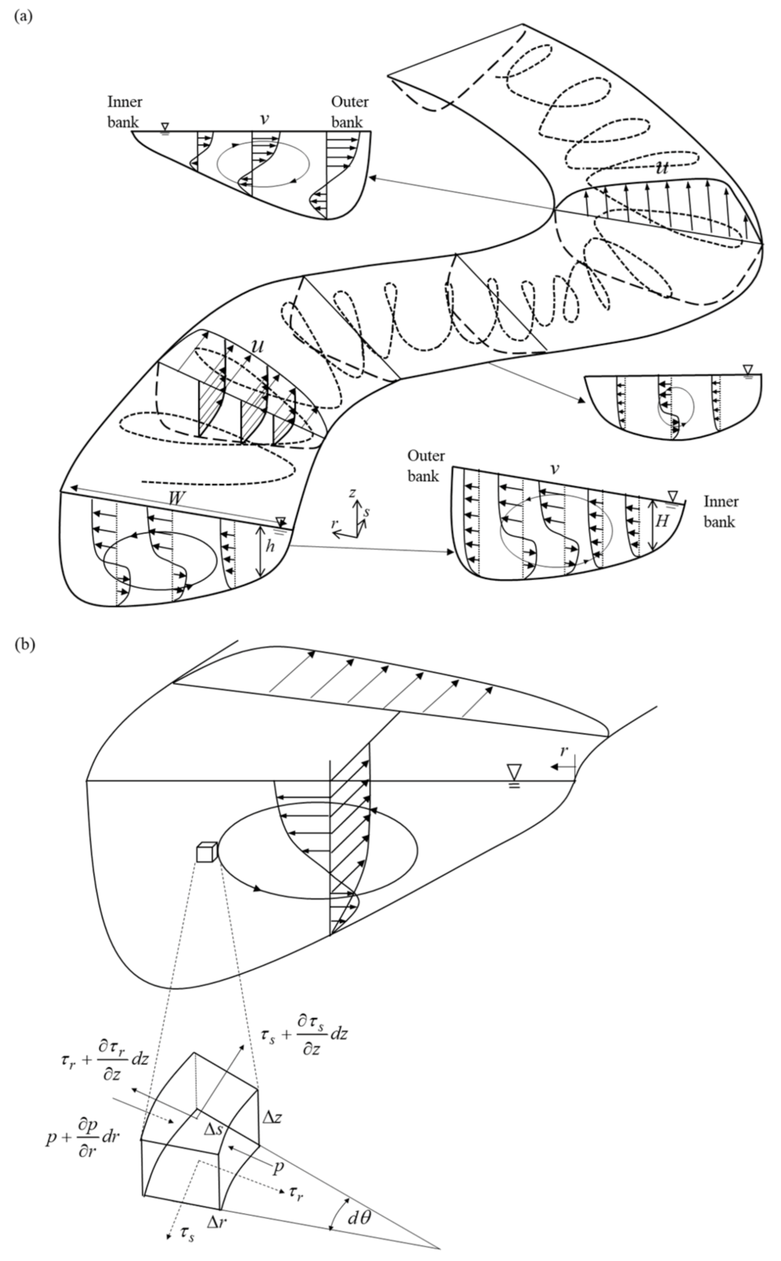
Modeling of the primary and secondary flows in a meandering channel is a challenge compared to straight channels, due to the complication in flow structures. Figure 1 shows that in curved channels, a helical flow structure is formed in the bend, in which the secondary flow evolves along the sinuous path of the channel. This secondary flow in meandering channels is caused by the local imbalance between the transverse water pressure forces generated by the super elevation of the water surface, and the vertically varying centrifugal force [1]. The local force imbalance causes a secondary cell to form, so that the lower part of the water column flows to the inner bank, while the surface part of the water column flows to the outer bank, which affects the local scouring and sedimentation occurring at the bend areas. Furthermore, the secondary flow affects the transverse dispersion rate through the mass and momentum redistribution from the helical flow structure. The advective momentum transport by the secondary flow also causes longitudinal velocity redistribution, in which the primary flow is shifted to the outer bank, as shown in Figure 1 [2]. Thus, understanding of the shear effect of the secondary flow in bends is necessary in order to analyze the transverse distribution of the longitudinal velocity, as well as to study the mixing of sediments and pollutants in meandering channels.
In the modeling of flow in meandering channels, although three-dimensional (3D) models showed the highest accuracy in reproducing the complex flow in curved reaches, 3D hydrodynamic models have some limitations due to their high computational requirements. Therefore, for the modeling of flow and mass transport in a relative shallow water system, such as open channels and rivers, 2D depth-averaged models may be more accessible for application. However, in the existing 2D numerical models frequently used in rivers, the depth-averaging sequence of 3D Navier–Stokes equations causes the loss of three-dimensional information in the momentum terms. This information can be partially retrieved by introducing the dispersion stress terms, which involves the integration of the discrepancy of the averaged and fluctuated transverse velocity in the momentum equations. In the dispersion stress method, the terms using vertical profiles of both longitudinal and transverse velocity were inserted, so the secondary current effect was included in the momentum equation [3]. Thus, in order to apply the dispersion stress method to the 2D depth-averaged momentum equation, vertical profile equations for both longitudinal and transverse velocities are needed.
Even though many researchers have studied the vertical profile of the transverse velocity in curved channels, most equations were derived by neglecting the nonlinear effects in the momentum equation. In sharp curvature channels, the secondary flow magnitude grows less linearly due to the nonlinear interactions between the longitudinal flow component and the secondary flow component [4], due to the advective momentum transport by the secondary flow, which flattens the downstream velocity profile. This leads to the secondary strength to decrease in the upper part of the water column and increase in the lower part of the water column, limiting the strength of the secondary flow. Rozovskii [5] and Kikkawa [6] derived the vertical profile equations of the secondary flow from the momentum equations using a logarithmic form assumption, without considering nonlinear relations between primary and secondary flows. To derive another secondary flow equation, the perturbation method was used by de Vriend [7] assuming the radius-of-curvature is smaller than the depth of the meandering channel. Since the former developed equations were still complicated, Odgaard [8] connected the vertical profile of the secondary flow to the surface velocity to create a linear profile. Although this was considered the easiest method for implementation, the simplicity was too high to account for the complex mechanisms of velocity deviations from the mean at the top and bottom parts of the vertical profile.
For the accurate representation of the secondary currents, the objective of this research is to develop a new vertical profile equation of the transverse velocity based on the experimental results, by considering the nonlinear relationship between the longitudinal and transverse flows, which was omitted in the previous equations. The dependence of the secondary flow on certain variables, such as the ratio of the depth over the radius-of-curvature, was analyzed using experimental results obtained from the meandering experimental channels. In this study, the proposed equation for the vertical profile of the transverse velocity was incorporated into the momentum equations of the 2D finite element model in the dispersion stress form, in order to reproduce the shear effect of the secondary current in the flow structures in modeling meandering channel flows.
2. Theoretical Studies
2.1. Two-Dimensional Flow Modeling in Meandering Channels
Many researchers have conducted two-dimensional modeling of shallow flow in a curved channel [9,10,11,12,13,14,15,16,17,18,19,20,21,22,23], in which they tried to include the effect of secondary flow on the primary flow behavior. To incorporate the effect of the secondary flow in the depth-averaged 2D model, several methods were proposed. Among them, two popular methods are the moment of momentum method and the dispersion stress method.
The moment of momentum method uses the 2D vertically averaged moment model (VAM), which was developed for the momentum redistributions. Originally, Johannesson and Parker [9] presented an analytical model to calculate the lateral distribution of the depth-averaged flow velocity in curved rivers. This made it possible to take into account the convective acceleration of the secondary flow that would suppress the growth of the primary flow. This became the basis of the later models of the moment of momentum method. The equations include the incorporation of the assumed distribution of vertical velocity components with vertical velocity and pressure distributions, which resemble transport equations.
Yeh and Kennedy [10] developed a moment model in which derivation involved a differential formulation in open channels to apply the secondary flow and the curvature effects to the transverse velocity profile. The research implied that the momentum calculation is important to explain the relations between the primary and secondary flow. Ghamry and Steffler [11] introduced the 2D VAM model, in which the depth-averaged continuity and momentum equations are coupled with additional moment of momentum equations, which were derived from the balance of the momentum flux of the convective terms, stress term, and pressure gradient term for secondary flow closure purposes. Vasquez et al. [12], who applied 2D finite element river morphology based on the VAM equations, maintained that their model was capable of reproducing the main effects of the flow in bends in a quasi-three-dimensional way. Using the original model developed by Ghamry and Steffler [11], the research showed that the model could be coupled with a bed load sediment model for morphodynamic applications. In contrast to former research, 2D research dealing with the convective acceleration of the secondary flow, such as the moment of momentum method [10,11,12,13], was conducted for better secondary flow estimation. However, since it involved the solving of several additional differential equations, the computational cost was expensive.
Another method is the dispersion stress method, which can be used in order to represent open flow in meandering channels where the vertical variations of the velocity would be re-applied, as it is usually omitted in the depth-averaging process. It is associated with the terms where the integration of the products of the fluctuating velocity components is directly calculated by incorporating the velocity vertical profiles of both the longitudinal and transverse velocities. By using the deviation between the depth-averaged and the actual velocity distribution, the neglected vertical variations are reassigned into the momentum equations of the 2D depth-averaged model. This approach is useful since it uses a vertical velocity profile without solving additional transport equations, which were introduced in the moment of momentum method.
Lien [3] developed a 2D depth-averaged model with the dispersion stress terms for simulating flow patterns in channel bends, in which the experimental data from Rozovskii [5] and de Vriend [7] were compared for model application, showing the secondary flow effect. This research showed that the dispersion stress term can play a major role in transverse convection of the momentum shifting from the inner bank to the outer bank. Bernard and Schneider [14] proposed a method to accurately reproduce the secondary flow that was measured in a bendway flume experiment to be included in the finite volume model STREMR. This method derived a transport equation for streamwise vorticity that considers the vorticity generation due to curvature to calculate the dispersion terms. Finnie et al. [15] used the method developed by Bernard and Schneider and applied it to a depth-averaged flow model, RMA2, a hydrodynamic finite element model. A transport equation for the streamwise vorticity was solved, and the results were converted into additional accelerations in the momentum equation. The dispersion stress term had an effect on the depth-averaged velocity calculations as the primary flow velocity size decreased on the inside and increased on the outside of the channel bends.
Begnudelli et al. [16] dealt with the 2D hydrodynamic numerical model by calculating the momentum equations that included dispersion stress terms. The dispersion stress term used a power-law for the longitudinal component, and the equation by Odgaard [8] was used for the transverse component which would account for the transfer of energy out of the circulating flows. Duan [17] also developed a 2D numerical model using the Odgaard [8] equation for transverse flow for the dispersion term calculations. The research maintained that the effect of dispersion stress terms became significant as the channel curvature increased. Song et al. [18] found the importance of the effects of the secondary current in a confluent channel and natural stream using the de Vriend equation [7] for the dispersion stress term. They stated that the pressure gradient terms of the momentum equations were the main factor that triggered the redistribution of longitudinal velocity. Yang et al. [19] studied the secondary flow effects in open channel confluence flow using dispersion terms in the momentum equation. They observed that the influence of dispersion terms would reflect the vertical non-uniformity of transverse velocity and the size of the separation zone. Akhtar et al. [20] simulated the curvilinear stretch in a natural river using a depth-averaged model with the dispersion stress term using the method similar to Duan [17], and found that as the sinuosity in the river increases, the effect of the tensor in the flow field increases, especially in channels with multiple meanders. Chen et al. [21] used the dispersion stress method similar to de Vriend (1977) for a laboratory curved channel, while Qin et al. [22] used a 2D depth-averaged model incorporating secondary flow to meandering experimental flumes, which used the methods by Lien [3], Bernard and Schneider [14], and later used these methods in another study [23], along with the method by Ottevanger et al. [24], to a natural channel to reflect the velocity redistribution. Nikora et al. [25] used extensive experimental results and modeling to find the size and effect of secondary current-induced dispersion stress in high Reynolds numbers.
The aforementioned models adopted vertical profile equations for the secondary flow into the dispersion stress term in 2D flow models to incorporate the secondary flow effects. However, the vertical profile equations in early research based their assumptions on mild curvature, so the nonlinear effects were usually discarded [5,6]; alternatively, the perturbation method in which the equation was limited to less sharp curves was applied [7]. Therefore, previous dispersion stress models incorporated with the existing secondary velocity profiles had the disadvantage that most models overestimated the effect of the secondary flow, especially in the case of sharp meanders [3]. Furthermore, usage of other dispersion stress models that calculated additional vorticity terms or Reynolds stress terms would be time expensive [14,16]. Thus, 2D modeling with a revised dispersion stress term is needed, in order to correctly represent the effect of secondary flows in both mild and sharp meandering channels efficiently.
2.2. Vertical Profile Equations for Secondary Currents
In previous research for the transverse velocity of secondary currents in meandering streams by Rozovskii [5], Kikkawa [6], and de Vriend [7], the depth was considered to be much less than the width and radius of the curvature. This allows the researcher to assume that the bank effects are minimalized in the equation derivation. They derived the circular form vertical profile from the momentum equations, with the upper part of the velocity profile moving to the outer bank, while the lower part of the profile moves to the inner bank, as shown in Figure 1. These research papers used the vertical profile equation directly for meander channel modeling, and can be described as linear secondary flow modeling. However, later research by Blanckaert and de Vriend [4,26], Ottavenger et al. [24], and Wei et al. [27] used non-linear secondary flow modeling, which showed that the interaction between the primary flow and secondary flow were important, since it would cause the overall decrease of the growth of the secondary flow strength.
Rozovskii [5] studied the flow in meandering open channels with several experiments, and summarized the results in the derived equations. One of the derived equations was the vertical distribution of fully developed transverse velocity, which was compared with data from a single bend experiment using growth and decay functions to show the changes and variance of secondary flow strength in meandering channels. The research assumed the logarithmic profile of the longitudinal velocity, then obtained the transverse velocity profile in the case of a smooth bed as follows:
where v is the transverse velocity, η is the dimensionless distance from the bed, H is the depth, ū is the depth-averaged longitudinal velocity, κ is the von Karman coefficient, C is the Chezy coefficient, RC is the radius of curvature, and g is the acceleration of gravity. This assumed that when the radius of curvature was many times larger than the channel depth, there was an equilibrium of the pressure force, centrifugal force, and turbulent shear stress.
Kikkawa [6] also developed the equation for transverse velocity from the equation of motion, assuming that the flow to be equilibrium and that the eddy viscosity is constant within the cross section of the channel and has a sufficiently large radius. The derived equation is:
where U is the cross-sectional averaged longitudinal velocity, is the radial distribution of the depth averaged velocity normalized by U, and is the cross-sectional averaged shear velocity with the following equation:
where Rh is the hydraulic radius and Sf is the friction slope of the channel. These equations show that the channel water depth, compared to the radius of curvature, has a linear effect on the secondary flow strength, which is similar to the Rozovskii equation.
Using the perturbation method, de Vriend [7] created a transverse velocity profile equation, in which the ratio of the depth-to-radius-of-curvature was selected as the perturbation parameter and the dependent variables of the equation were expanded in a power series. This allowed the higher order terms of the second order to be neglected for obtaining the solution. Using the depth-averaged model to simplify the three-dimensional meandering channel into a two-dimensional problem, it has the secondary flow and main flow functions Fs and Fm, respectively:
where Un is the Euclidian norm of longitudinal velocity and rψ is the local radius of the curvature in the streamline system. This equation shows that the logarithmic profile of the longitudinal flow could affect the characteristic and shape of the secondary currents.
Odgaard [8] considered the velocity profile of the secondary flow cell as a circular motion type, and introduced a linear transverse velocity profile using this presumption with the following equations:
where = depth-averaged transverse velocity, us = transverse velocity at the water surface, and . This equation utilizes the longitudinal velocity at the water surface. With this equation, the author developed a 2D model for simulating the flow and bed topography in a meandering alluvial channel.
Baek et al. [28,29] used the linear profile of Odgaard [8] to derive the longitudinal variation of transverse velocity along sinuous channels with alternating bends. Seo and Jung [30] compared several theoretical velocity distribution profiles of secondary currents with experimental data from a sinuous channel experiment, and showed that the increase of sinuosity tends to enlarge the deviation of the transverse velocity.
However, as aforementioned, nonlinear terms that account for interactions between the primary flow and secondary flow were neglected by those researchers when they derived the equations of the transverse velocity. The nonlinear terms that account for interactions between the primary flow and secondary flow needed to be reflected to accurately portray the vertical profile of the secondary flow depicted as in Figure 2. The outward centrifugal acceleration and the pressure gradient due to the superelevation causes the secondary flow. With nonlinear behavior, the centrifugal acceleration is reduced due to the advective momentum transport flattening the velocity profile, causing the secondary flow to decrease in the upper part of the water column.
Blanckaert and de Vriend [4] demonstrated that the curvature-induced secondary flow was caused by the combination of outward centrifugal force and inward pressure gradient. In mild curved channels, interactions between the longitudinal and transverse flow would be small, and the secondary flow would increase linearly with H/Rc. However, nonlinear behavior by the sharper curves or the history affect by multiple meanders would cause the decrease and irregularity of the outward centrifugal force, which would then lead to the overall decrease of secondary flow strength at the top and bottom parts of the water flow. Ottavenger et al. [24] used the model to show how the nonlinear secondary flow affects the bed morphology in sharp bends with coupling, and the nonlinear model had better results compared to the linear model, which over-predicted the transverse bed slope gradients.
In this regard, Wei et al. [27] also showed that the commonly used linear models, in which secondary current effects linearly depend on the H/Rc, may overestimate the strength of the curvature inducement. Thus, following the research by Blanckaert and de Vriend [4], they introduced a nonlinear method concerning the term as the major control parameter, using the depth over the radius-of-curvature ratio and the dimensionless Chezy friction coefficient, , which is given as . Wei et al. [27] used the nonlinear model to find the dependence of secondary flow strength on the H/Rc parameter in bends with laboratory experiments with various H/Rc terms. Even though their equations showed better application to sharp curvature flows, the equations were rather complex and validations were limited to single bend flows and laboratory experiments.
Thus, in this study, existing equations for the vertical profile of secondary currents were tested using comprehensive experimental data obtained in the meandering channels with sharp curvature flows and multiple bend flows. A simpler equation in which the nonlinear term was sustained to include the effect of advective momentum was proposed, and incorporated into the 2D shallow water model via the dispersion stress method.
2.3. Derivation of the Vertical Profile of the Secondary Currents
In this study, the development of the transverse velocity equations was first based on the 3D Navier Stokes equation in cylindrical coordinates, as shown in Figure 1. The equations of motion for longitudinal and transverse velocities are given as [31,32]:
where u, v, w are the velocity components of the s, r, z directions for the cylindrical coordinates, respectively, r is the transverse coordinate point, ρ is the water density, Sr is the transverse water surface slope, s is the longitudinal water surface slope, and are the shear stresses in the s and r directions, respectively shown as:
where ε is the eddy viscosity. Using the assumption of steady and developed flow, and the logarithmic law for the vertical velocity profile, longitudinal velocity in a cross-section was derived combining Equations (15) and (17), as below:
where α is the correction term introduced to account for the nonlinear behavior and . Then, Equation (16) can be integrated by using Equation (19) for the longitudinal velocity and using the boundary condition in which friction on the free surface equals zero. The result of the integration of Equation (16) is the following:
In this study, for the applicability of the developed equation, the α coefficient was introduced for nonlinearity, which would be based on the experiment data, and used in the form of , where ω is a coefficient that would be calibrated with the secondary current measurements from the channel. This enabled the equation to limit the growth of the secondary flow in the top and bottom layers of the water flow in sharper curvatures. Furthermore, in this study, by considering the sensitivity of the depth over the radius-of-curvature ratio, the H/Rc term was changed to a non-dimensional factor for the exponent using the measured data from the experiment; the final form of the vertical profile for the secondary flow then became the following:
3. Experiments
3.1. Acquisition of the Field Data
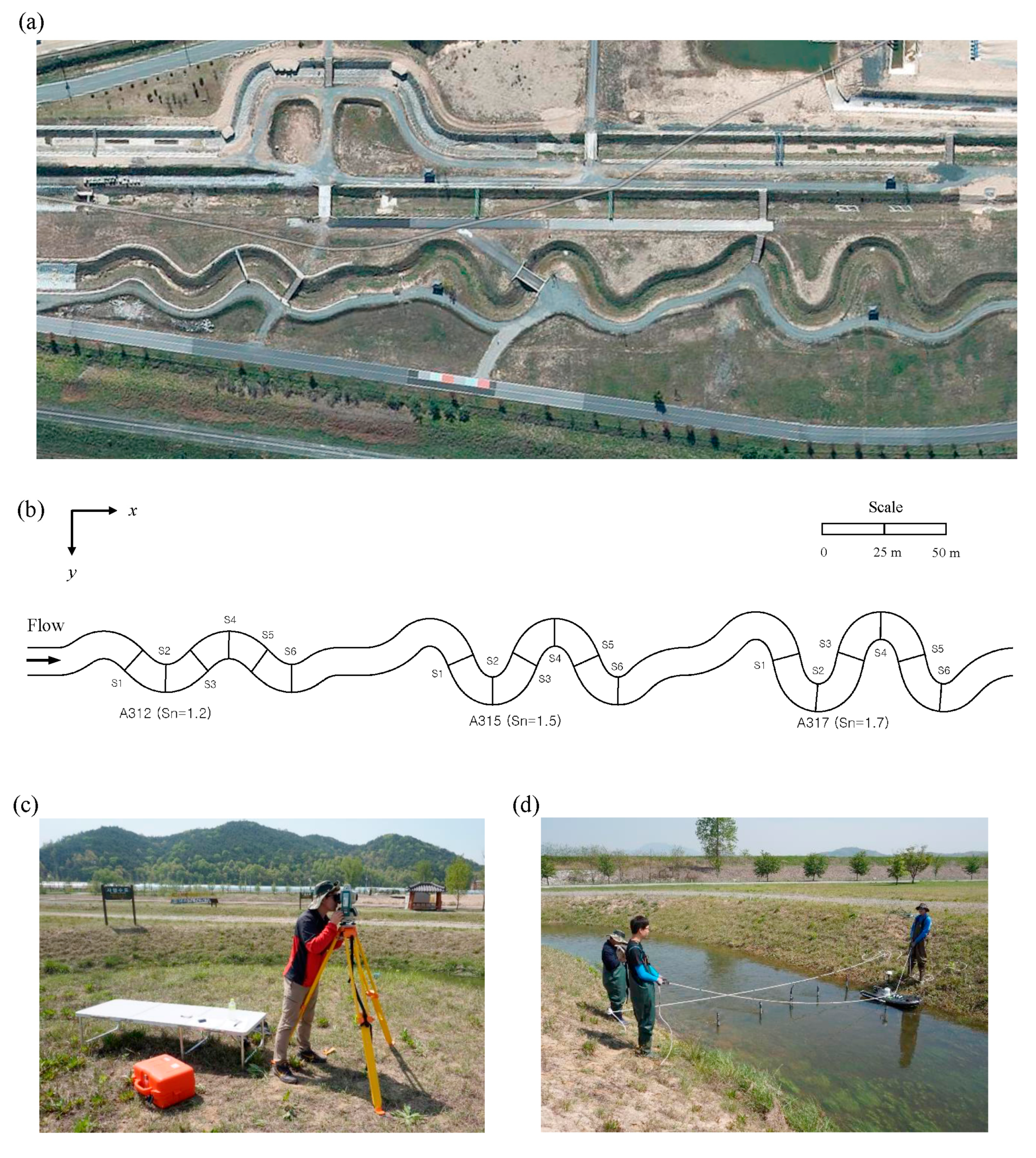
To find the effects of the secondary current in meandering channels, a series of large-scale channel experiments were conducted at the River Experiment Center (REC) of the Korea Institute of Civil Engineering and Building Technology (KICT) located in Andong, South Korea. A real-size meandering channel was installed in order to simulate open channel flows in a controlled outdoor environment. The meandering flume is about 11 m wide and 600 m long, with reaches of three different sinuosities, as shown in Figure 3. The full discharge capability of the REC channel is 10.0 m2/s, using large pumping facilities which draw their water from the nearby Nakdong River. This makes it possible to conduct various river experiments almost free from scale effects. The experiments were conducted to obtain the velocity data needed for the creation of a vertical profile equation for the secondary current, and for the validation of the 2D numerical model incorporated with the proposed dispersion stress module. Table 1 describes the experiments.
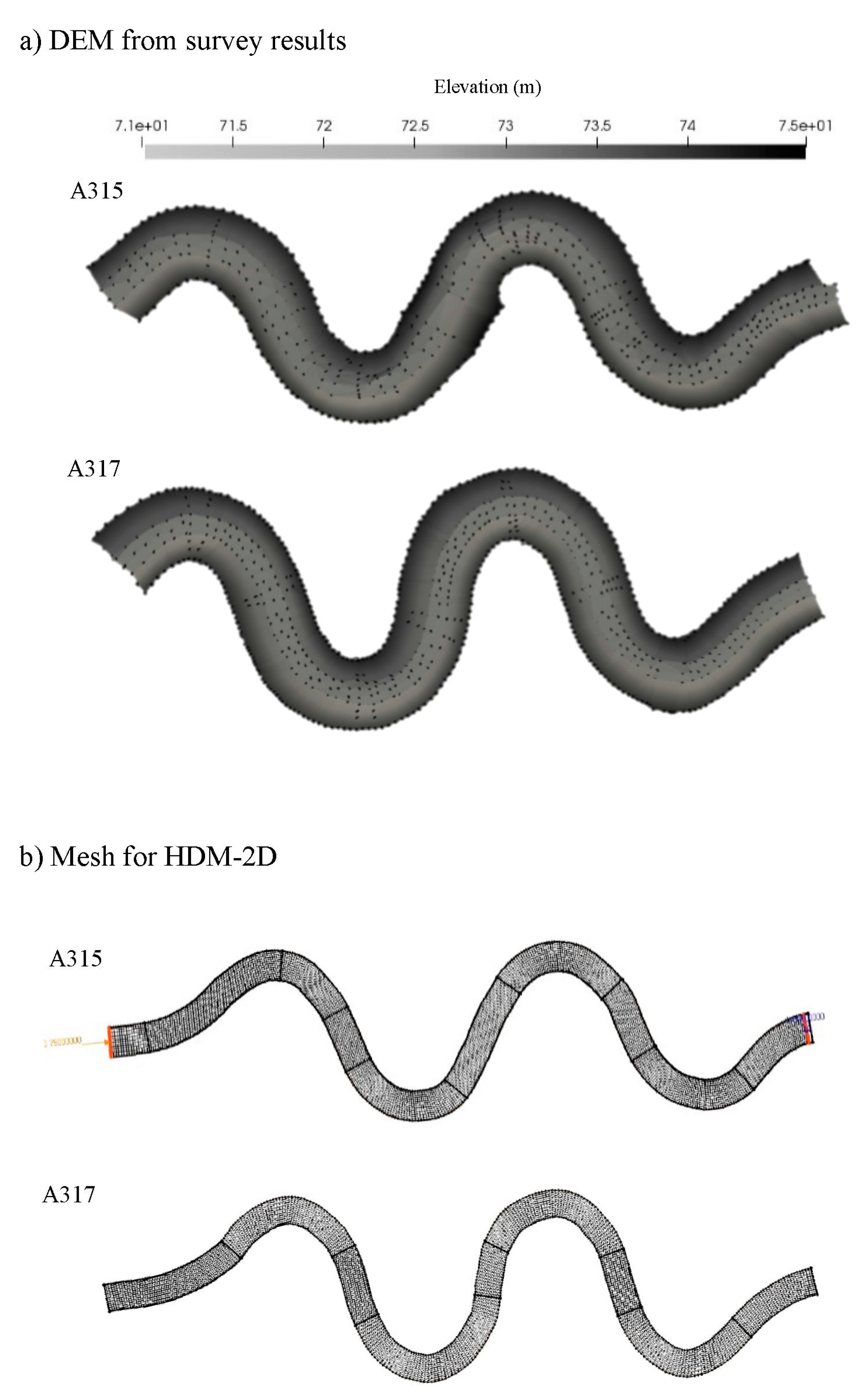
A topography survey was first done with the total station and RTK-GPS for point measurements, as shown in Figure 3c. Then, drone-captured aerial photography for the surface elevation was conducted for interpolation between the surveyed points. Structure-from-Motion was used by the Pix4D program for the surface elevation points [33]. Figure 4a is the result of the total station and RTK-GPS point measurements to show the topography of the meandering channels, and coordinates of the ground control points installed at 12 points over the channel were later used with the drone-captured aerial images to compute the topography. Although the meandering channel was originally constructed to be a trapezoidal section, continuous experiments caused the channel to change to a more natural form with erosion and deposition around the banks, as shown in Figure 4a. Later, the mesh generation of the meandering channel was completed using the surface elevation map as shown in Figure 4b.
The flow velocity measurements were conducted with an Acoustic Doppler Current Profiler (ACDP) and Acoustic Doppler Velocimetry (ADV). The ADCP used in this study was the SONTEK S5, a multi-band acoustic frequency capable model with profiling ranges up to 0.06 to 5 m depth and velocity up to 20 m/s [34]. The flow experiments were first conducted with an ADCP, which was operated on the moving boat connected to a tether line as shown in Figure 3d, while the channel width during the experiment was about 5–6 m. The ADCP boat was operated six times per section, so the measurements were taken three times per direction for averaging. Three-dimensional velocity and bathymetry data were obtained at six cross-sections distributed throughout each meandering channel. Half of the cross-sections were placed at the apex of curvature, and the other half between the apexes of the meandering channels as shown in Figure 3. Cross-sections were placed with tag lines at a distance of 30–50 m each. The flow characteristics were measured at each section of the channels, to find out the characteristics of the primary flow distribution and the secondary flow structure.
3.2. Data Analysis of Secondary Currents in the Meandering Channels
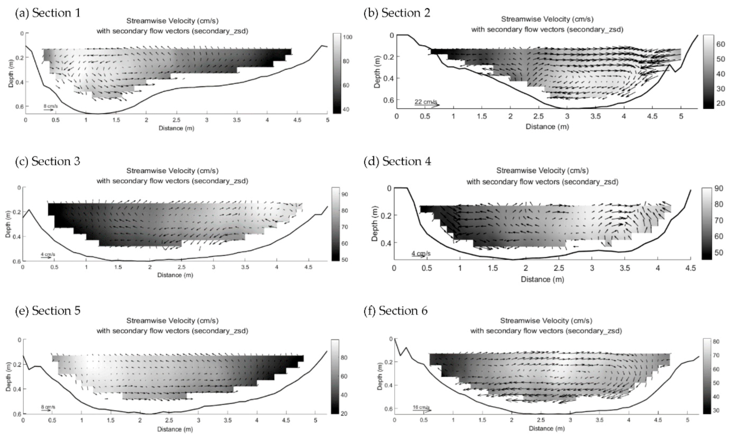
The Velocity Mapping Toolbox (VMT), an ADCP post-processing software package based on a MATLAB-based toolbox [35], was used to obtain spatially and temporally averaged velocity data for each cross-section from repeated sectional measurements of 3D velocities. Figure 5 shows the velocity contours of the temporally averaged longitudinal velocity, along with secondary currents at bends and straight sections of Case A3-E21. The measured data can be interpolated to grid nodes using a least-squares regression line fit through transects at each cross-section with the velocity ensembles. The measured velocity components were used to derive the depth-averaged vector plots of longitudinal and transverse velocities for the individual cross-sections. To identify the secondary flow structure formation within complex meandering flows at the channel, the program also rotates the velocity vectors for each line in an ensemble to the direction of the depth-averaged velocity vector. Secondary flow is then defined by velocity components perpendicular to this rotation, as depicted in Figure 1b. Previous studies of river hydrodynamics have used this rotation method to detect helical motion in strongly converging flows [36,37].
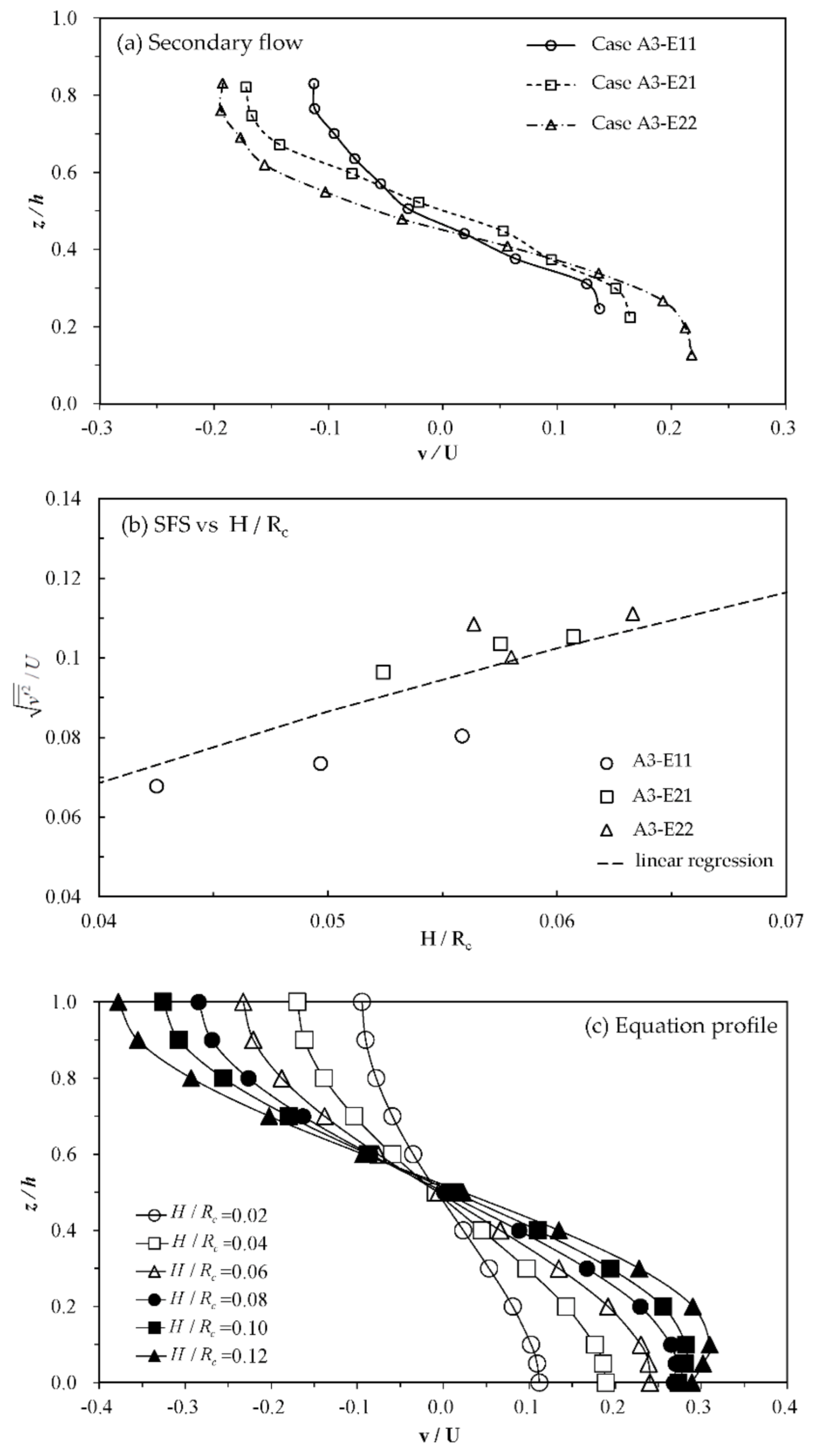
Figure 6a shows the measured secondary current results in meandering channels with different sinuosities, and these results revealed that as the sinuosity increases, the strength of the secondary flow increased. Figure 6b shows the relations between the secondary flow strength and the ratios of the depth over the radius-of-curvature using the experimental results. In this figure, the non-dimensional index of the shear intensity of the secondary flow (SFS) is defined as:
where v′ is the deviation of the transverse velocity at vertical position from the depth-averaged transverse velocity. This figure shows that the relations are not an exact linear pattern, and the power form would be an acceptable choice in the description of the relationship. These experimental results suggest that in order to represent the effect of secondary currents in the curved channel, the new equation for the vertical profile of the secondary flow should include H/Rc.
3.3. Validation of Transverse Velocity Profile
In this study, the coefficients α and β of Equation (20) were found based on the measured experimental data; constant β was determined to be 0.935 from the relation between secondary flow strength and the depth over radius of curvature results shown in Figure 6b. The coefficient ω from was determined to be 20 through comparisons with the measured velocity data, and affected the term of the proposed equation for the vertical profile. This enabled the vertical velocity profile to be more applicable to channels with various curvatures, especially channels with high sharpness and multiple meanders.
For closer analysis and investigation of the effects of the H/Rc on the proposed equation for secondary flow velocity, the H/Rc term was increased in increments to find the relation to the size of the secondary flow. Figure 6c shows the higher H/Rc to increase the size of the secondary flow. Note that as the depth-to-radius-of-curvature ratio increases, the growth of the secondary flow size is limited in the top and bottom parts of the vertical profile when using the secondary flow equation to reflect the nonlinearity shown in the experimental channels. This is due to the coefficient introduced in the proposed equation, which serves as a coefficient to reflect the gradual damping in the secondary flow strength as it increases with the depth-to-radius-of-curvature ratio. This state can also be seen in Figure 6b, as the SFS is plotted with H/Rc, which shows some nonlinear attenuation of the secondary flow strength as H/Rc increases to a value higher than 0.06, as opposed to the linear regression line. The secondary flow would cause the decrease of the longitudinal flow by nonlinear behavior caused by strong secondary flows or a history effect in multiple meanders, which affects the outward centrifugal force; then, the irregular decrease of the centrifugal force will cause the decrease of secondary flow strength in the top and bottom parts of the water flow. Figure 6c shows that the proposed secondary flow equation can reflect the nonlinear behavior in sharp channels to represent the attenuation of the shear effect of the secondary current in the sharp-curved channels, which was depicted in Figure 2.
To find the acceptability of the transverse velocity profiles, the proposed equation was compared with the experimental data of the REC meandering channel. Figure 7 shows the comparison with the experimental data of A315 channel and Table 2 lists the average root-mean-square errors (RMSE) of the proposed equation and existing equations. Table 2 shows that the proposed equation in this study shows the least RMSE for all cases of the meandering channels. Figure 7 reveals that the proposed equation shows better fit in the top and bottom layers of the secondary flow of the vertical profile in full sized experiments with multiple curves, while the other equations show overestimation at the points. This was possible since a nonlinear term was reflected in the proposed equation, and the multiple curves caused a history effect, where the secondary cell that developed at the former bend in the opposite direction had not completely disappeared at the next bend, as sketched in Figure 1a.
4. Model Applications
4.1. Development of the 2D Numerical with the Dispersion Stress Term
In this research, the proposed equation for the secondary flow was inserted into a dispersion stress form of the 2D finite element solver HDM-2D, a depth-averaged numerical model that was originally developed by Seo and Song [3]. In HDM-2D, the streamwise upwind Petrov–Galerkin stabilization approach from the finite element method was used to solve the unsteady two-dimensional depth-averaged flow equations. The Galerkin method of weighted residuals solves the weak form of the boundary value problem after multiplying the shallow water equations by a weighting function, and uses Green’s theorem to integrate the weak form over the flow domain. Then, the results are time-discretized with a fully implicit method. Finally, the shallow water equations are formed with a non-conservative form that considered the stability of schemes. The non-conservative form yields the simpler form of the viscous terms and the upwinding procedure for convective terms is straightforward, depending on the velocity direction (Agoshkov et al., 1993) [38]. The HDM-2D used in this research uses the momentum equation with the dispersion stress term in tensor form, as below [3,18,39]:
where are the velocity in the x and y directions, respectively, in Cartesian coordinates, are the depth averaged velocity in the x and y directions, respectively, z is the bottom elevation, is the kinematic eddy viscosity coefficient, n is the Manning coefficient, and is the dispersion stress term. The momentum equations were discretized by the SU/PG scheme with an element characteristic length shown by Yu and Heinrich [40,41]. The eddy viscosity was calculated using the Smagorinky eddy viscosity model [42], which had sufficient diffusion and dissipation to stabilize the numerical computations. Additionally, this study decomposed the velocity components into depth-averaged velocities and their deviations, and inserted them into the integration of the products of the velocity fluctuation of Equation (26). The proposed equations of the velocity deviation that were derived in natural coordinates were changed into Cartesian coordinates by the following equations:
where are the longitudinal and transverse velocity deviation components in Cartesian coordinates, respectively, are the unit normal vector for the longitudinal and transverse directions, respectively, and Fm and Fs are the longitudinal and secondary flow functions, respectively.
The above equations, Equations (27) and (28), change the flow in the longitudinal direction due to the influence of the secondary flow included in the second terms. This study used the logarithmic equation by de Vriend [7] of Equation (8) for the profile of the longitudinal flow Fm, while applying the proposed profile of the transverse velocity of this research by using Equation (30) for Fs, which was different from the secondary flow equation by de Vriend, which was used by the original HDM-2D [18]:
The relations for the depth-to-radius-of-curvature ratio were applied to the proposed transverse flow equation, which was then applied to the dispersion stress model. In this way, the nonlinear effect was included in the secondary current.
4.2. Validation Using the Rozovskii Channel
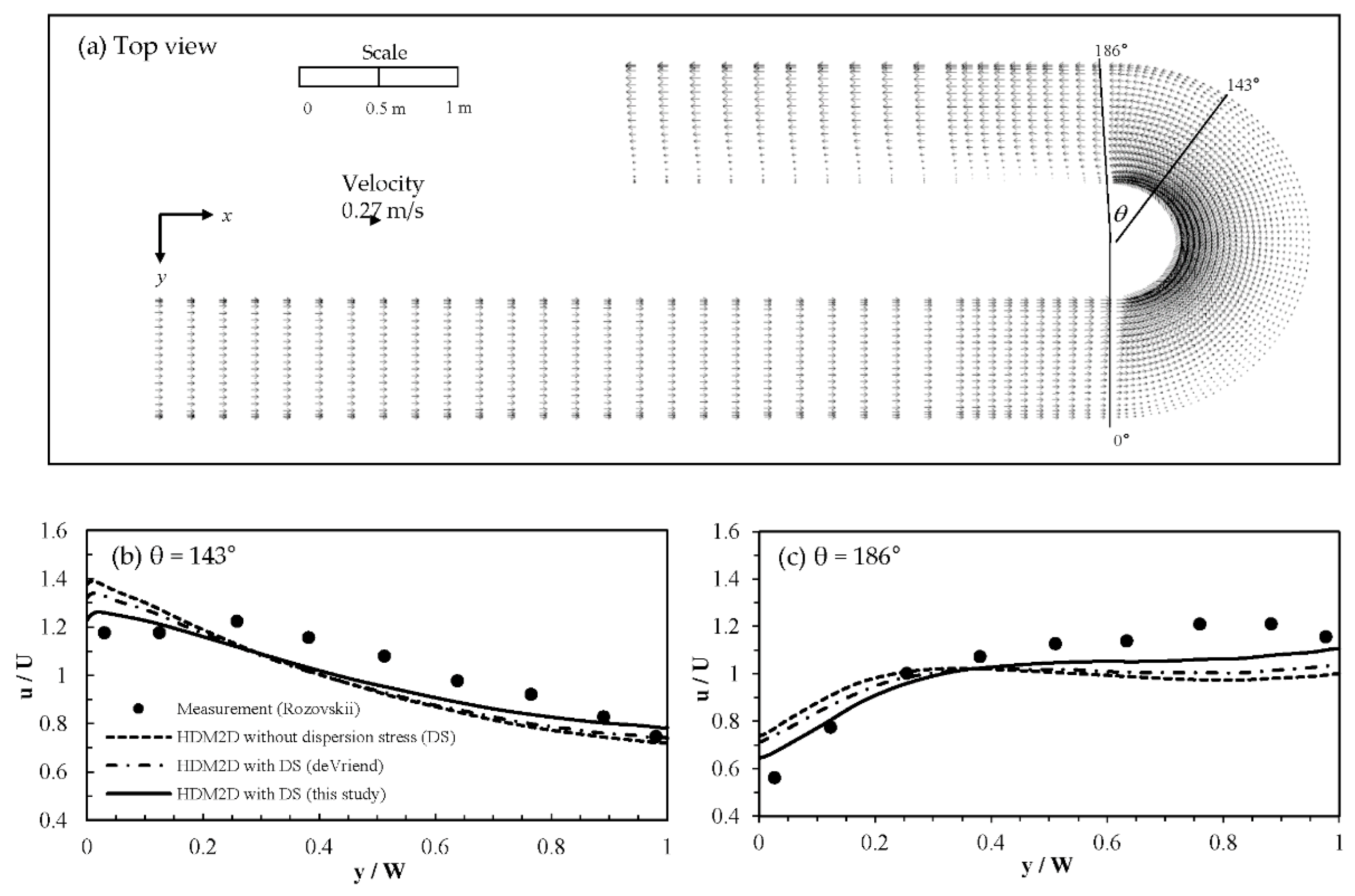
For the validation of the model, the experiment data obtained by Rozovskii [5] were used in a U-curved channel. Rozovskii [5] collected the velocity data in a sharp bend channel, in which the ratio of the width to the mean radius-of-curvature was 1.0, as shown in Figure 8a. It was expected that the experimental results in this channel would exhibit highly 3D flow characteristics, because it was a curve with a width-to-mean-radius ratio of 0.4 and more, which was considered to be sharp. The cross-section of the bend was rectangular, and connected to straight inlet and outlet reaches of the same cross-section. The approach channel was 6 m long, while the exit channel was 3 m long. The entire channel was horizontal with a 180-degree bend. The discharge in the channel was 0.0123 m3/s, and the water depth was 0.6 m.
This experiment showed that there is a gradual increase of transverse circulation at the entrance portion of the bend, and a similar decrease at the second half of the bend followed by more decay of the secondary flow at the straight run part of the bend, shown in the velocity distribution results in Figure 8. The simulated results contained the super-elevation of the flow as it goes through the sharp bend. Figure 8a shows that when the flow enters the bend, the velocity at the inner bank becomes larger, and the velocity at the outer bank becomes smaller. Then, the simulated velocity profile becomes uniform, later the outer bank velocity becomes larger with distance from the downstream of the bend exit.
Figure 8b,c indicate that due to the secondary flow effect, the velocity distributions change through the bend as the flow enters. The figure shows the results at degrees of 143 and 186, where the secondary current is fully developed and exits out of the bend. This validation conducted comparisons between the experiment results, a model without dispersion stress terms, and models using dispersion stress terms using three different equations that have linear and nonlinear effects. The linear dispersion stress model using de Vriend’s [7] velocity equation, which excluded the nonlinear effects, seems to overestimate the secondary flow influence in the channel. Additionally, the dispersion stress method that was implemented using the de Vriend equation [7] in the original HDM-2D displays less changes to the primary flow distribution compared to the proposed model in this study. This is shown in Table 3, where the de Vriend equation application had a bigger mean absolute percentage error (MAPE) than the proposed model. The results show that the primary flow distribution can be better reproduced by the proposed model than the simulations without the dispersion stress term or the simulations with the linear dispersion stress term.
4.3. Validation Using REC Meandering Channel Data
The dispersion stress model incorporated with the proposed velocity profile was tested against the experimental data obtained from the REC meandering channel. Both river survey data and the depth data measured using ADCP were used for the mesh generation of the 2D numerical model HDM-2D. Since the measurements were taken as a continuous boat-moving area, the averaging of the sections was done by spatial averaging, with a span and width interval of 0.1 m.
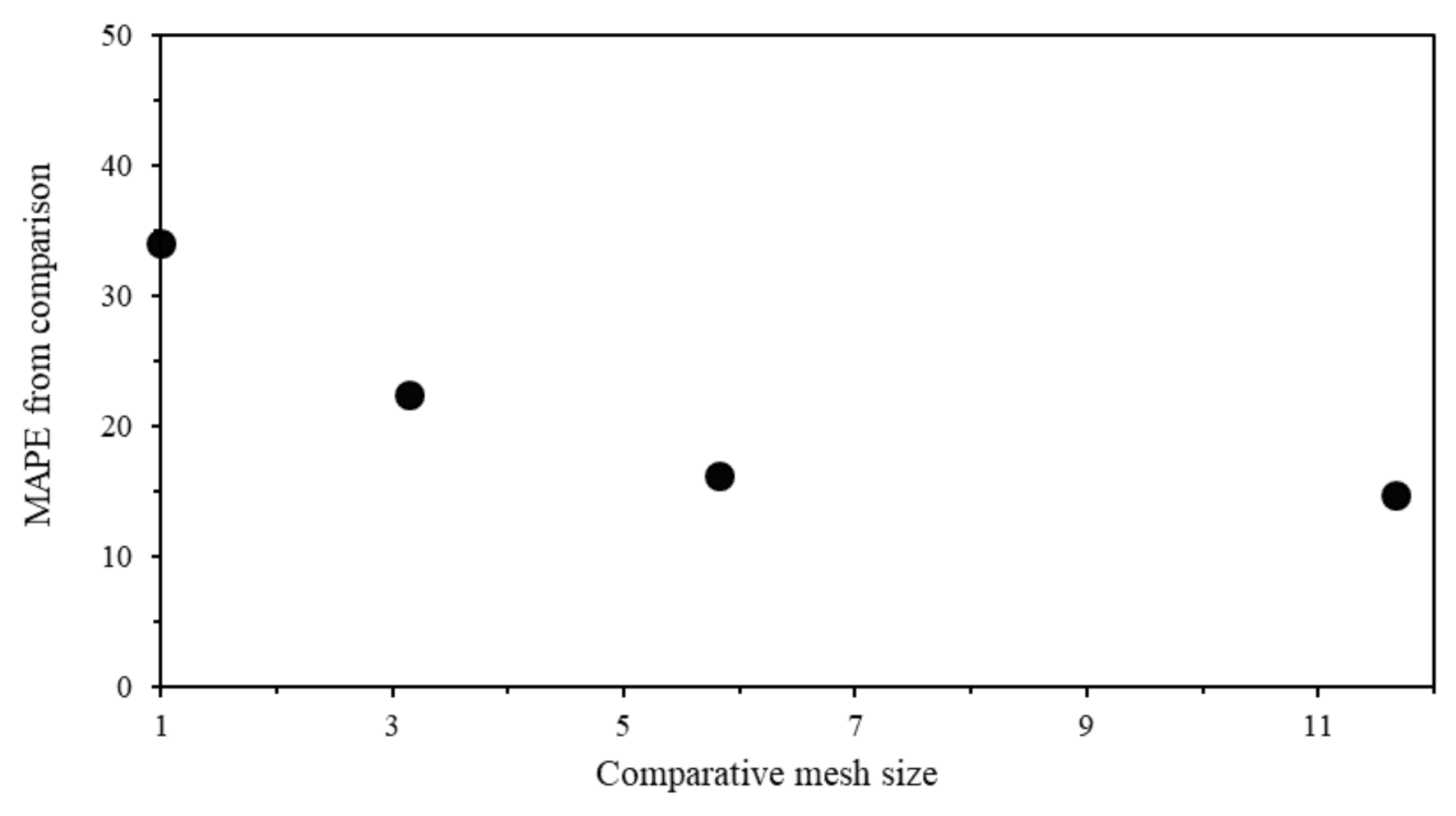
Before applying the dispersion stress, grid refinement was implemented to decrease the numerical errors so it would be relatively smaller than the flow modeling error results. The mesh was separated into four cases that had a very fine, fine, medium and the coarsest grid. The results of the errors for the comparison between the simulated results and ADCP measurements are shown in Table 4 and Figure 9 with the node size and MAPE results. Using a grid refinement ratio of over 2, the results show that the error between the very fine and fine grid was less than 1.4%, even with double the mesh size. From the grid refinement result, the very fine grid was determined to be suitable for continuous modeling for the experimental channel.
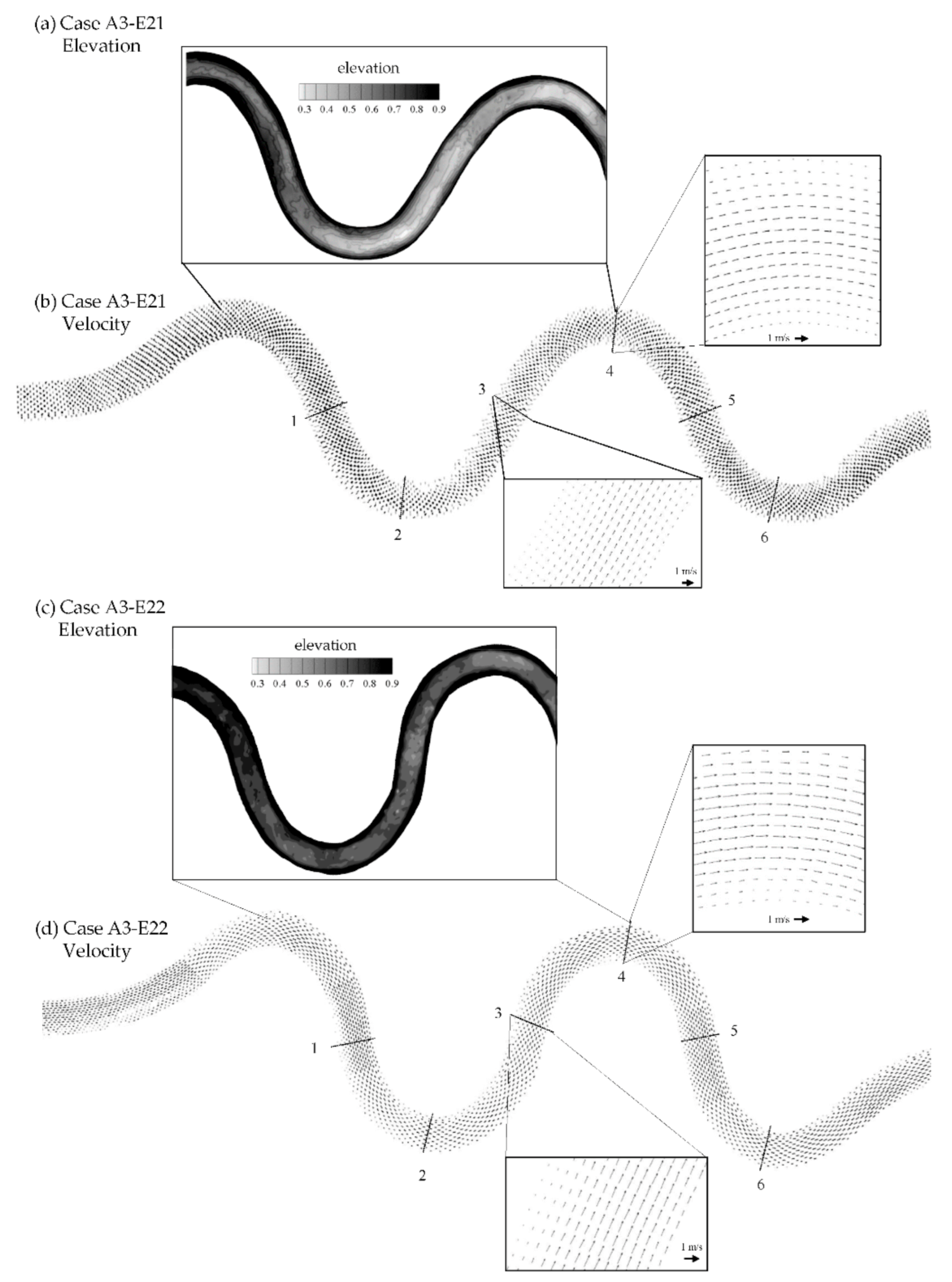
To find the effect of the dispersion stress on the flow modeling, the experimental results were compared with the modeling results that had the dispersion stress term and no dispersion stress term. The maximum primary velocity was developed along the thalweg line, and most of the even number sections located at the apex had the primary velocity distribution skewed toward the outer bank due to the secondary flow effect, as shown in Figure 10b,d. For the odd number sections, the position of the maximum primary velocity was affected by the upstream section, due to the history effect of the secondary flow. This history effect was considered to have arisen by the phase lag between the channel centerline and the discharge centerline or thalweg line [32].
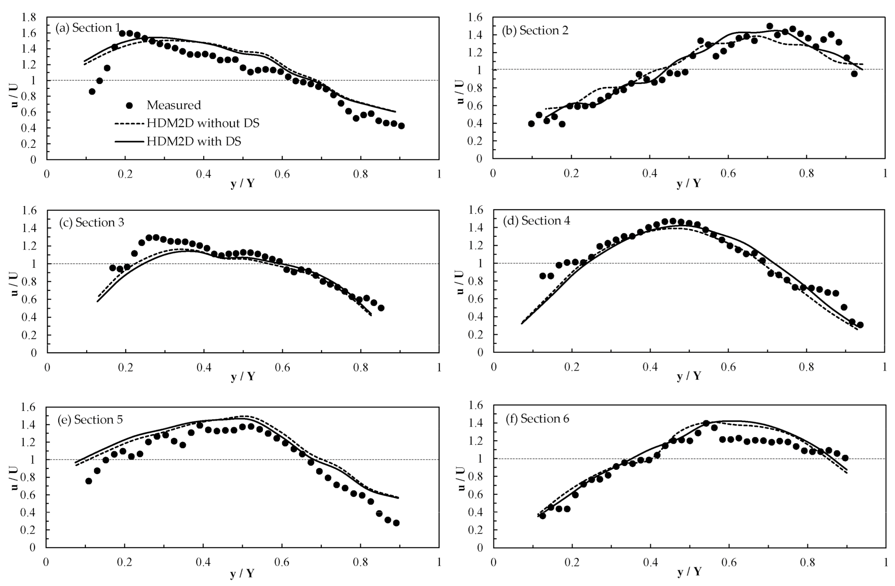
Figure 11 shows comparisons of the simulation by HDM-2D model with the measured data, in order to closely demonstrate the applicability of the dispersion stress term with the proposed equation to the transverse velocity. For the A315 channel, agreements between the measured data and the simulation are generally good. The HDM-2D models with the dispersion stress terms included produced the primary flow distribution that would be closer to the measured experimental results, which was more skewed towards the outer bank. Table 5 summarizes the results’ of the goodness of fit between the experimental data and the numerical simulation shown with the mean absolute percentage error, which was done specifically at the meander apex of the bends. These results showed that the original model had errors of 12.9%, while with dispersion stress, the error decreased to 10.4%, relatively 19% lower compared to the simulation without dispersion stress. The dispersion stress term skewed the primary distribution toward the outer bank in the apex sections, which is similar to the measured results. Overall, the results show that the dispersion stress model with the proposed velocity profile could reproduce the secondary current effect in sinuous channels quite accurately.
5. Conclusions
In this study, large-scale experiments were conducted in the KICT REC meandering channels to find the nonlinear effect of the secondary current on the primary flow distribution. The experimental results found the relations of the secondary flow strength to the depth over the radius-of-curvature ratio of the channel. Then, the vertical profile equation for the secondary flow was developed to reflect the nonlinear effects on the secondary flow. The proposed equation generated a vertical profile that showed a decrease in the maximum secondary flow strength at the top and bottom of the profile, compared to the existing equations which omitted the nonlinear effects.
The proposed velocity profile equation was inserted into the momentum equations with the dispersion stress method in order to induce the nonlinear shear effect of the secondary flow, which is normally neglected in the depth averaging process. The simulation results using the proposed equation to the dispersion stress method for the two-dimensional flow solver HDM-2D showed that the simulation of the Rozovskii channel produced improvement over the dispersion stress model using de Vriend’s velocity equation, which was based on the linear behavior between the secondary flow and primary flow as well as over the non-dispersion stress results in the distributions of the primary flow velocity. The validation results with REC meandering channels revealed that the 2D hydrodynamic model with nonlinear dispersion stress term gave a better fit to the experimental data than the simulation without the dispersion stress term by decreasing the relative error by 19%. The effect of the channel sinuosity was adequately represented by adopting the proposed nonlinear velocity profile into the dispersion stress term of the HDM-2D model. This effect of the sharp bend on the vertical profile of the secondary flow and secondary flow strength was further illuminated by comparisons with increasing depth over the radius-of-curvature ratios. The proposed equation incorporating nonlinearity showed the limitations of the growth of the secondary flow strength. These results confirm that the two-dimensional model HDM-2D with dispersion stress using the proposed velocity profile proves useful for assessing the secondary flow effect in meandering channels with the history effect of multiple bends, as well as in sharp curved channels where 3D spiral motions are predominant.
Author Contributions
Conceptualization, J.S. and I.W.S.; Funding acquisition, I.W.S.; Methodology, J.S. and I.W.S.; Project administration, I.W.S.; Software, J.S.; Validation, J.S.; Visualization, J.S.; Writing—original draft, J.S. and I.W.S.; Writing—review and editing, J.S. and I.W.S. All authors have read and agreed to the published version of the manuscript.
Funding
This work is funded by the Ministry of Land, Infrastructure and Transport, grant number 21DPIW-C153746-03.
Institutional Review Board Statement
Not applicable.
Informed Consent Statement
Not applicable.
Data Availability Statement
The data presented in this study will be shared by the authors if requested.
Acknowledgments
This work is supported by the Korea Agency for Infrastructure Technology Advancement (KAIA) grant funded by the Ministry of Land, Infrastructure and Transport (Grant 21DPIW-C153746-03). This research work was conducted at the Institute of Engineering Research and Institute of Construction and Environmental Engineering in Seoul National University, Seoul, Korea. The authors would like to express gratitude towards the Changwon National University, the United States Geological Survey, and the Seoul National University team for acquiring the experimental data, and Donghae Baek and Paul Kinzel for processing the surface elevation points from the topography data.
Conflicts of Interest
The authors declare no conflict of interest.
References
- Henderson, F.M. Open Channel Flow; MacMillian Publishing Company: New York, NY, USA, 1966. [Google Scholar]
- Blanckaert, K.; Graf, W.H. Momentum transport in sharp open-channel bends. J. Hydraul. Eng. 2004, 130, 186–198. [Google Scholar] [CrossRef]
- Lien, H.C.; Hsieh, T.Y.; Yang, J.C.; Yeh, K.C. Bend flow simulation using 2D depth-averaged model. J. Hydraul. Eng. 1999, 125, 1097–1108. [Google Scholar] [CrossRef] [Green Version]
- Blanckaert, K.; de Vriend, H.J. Meander dynamics: A nonlinear model without curvature restrictions for flow in open-channel bends. J. Geophys. Res. Earth Surf. 2010, 115. [Google Scholar] [CrossRef] [Green Version]
- Rozovskii, I.L. Flow of Water in Bends of Open Channels; Academy of Science of Ukrainian SSR: Moscow, Russia, 1957. [Google Scholar]
- Kikkawa, H.; Ikeda, S.; Kitagawa, A. Flow and bed topography in curved open channels. J. Hydraul. Div. 1976, 102, 1327–1342. [Google Scholar] [CrossRef]
- de Vriend, H.J. A mathematical model of steady flow in curved shallow channels. J. Hydraul. Res. 1977, 15, 37–54. [Google Scholar] [CrossRef]
- Odgaard, A.J. Meander flow model. I: Development. J. Hydraul. Eng. 1986, 112, 1117–1136. [Google Scholar] [CrossRef]
- Johannesson, H.; Parker, G. Secondary flow in mildly sinuous channel. J. Hydraul. Eng. 1989, 115, 289–309. [Google Scholar] [CrossRef]
- Yeh, K.C.; Kennedy, J.F. Momentum model of nonuniform channel bend flow I: Fixed beds. J. Hydraul. Eng. 1993, 119, 776–795. [Google Scholar] [CrossRef] [Green Version]
- Gharmry, H.K.; Steffler, P.M. Two dimensional vertically averaged and moment equations for rapidly varied flows. J. Hydraul. Res. 2002, 40, 579–587. [Google Scholar] [CrossRef]
- Vasquez, J.A.; Millar, R.G.; Steffler, P.M. Vertically-averaged and moment of momentum model for alluvial bend morphology. In Proceedings of the 4th IAHR Symposium on River, Coastal and Esturarine Morphodynamics, Urbana, IL, USA, 4–7 October 2005; Taylor & Francis: London, UK, 2005; pp. 711–718. [Google Scholar]
- Jin, Y.C.; Steffler, P.M. Predicting flow in curved open channels by depth-averaged method. J. Hydraul. Eng. 1993, 119, 109–124. [Google Scholar] [CrossRef]
- Bernard, R.S.; Schneider, M.L. Depth Averaged Numerical Modeling for Curved Channels; Technical Report HL 92-9; US Army Corps Engineers: Washington, DC, USA, 1992. [Google Scholar]
- Finnie, J.; Donnell, B.; Letter, J.; Bernard, R.S. Secondary flow correction for depth-averaged flow calculations. J. Eng. Mech. 1999, 125, 848–863. [Google Scholar] [CrossRef]
- Begnudelli, L.; Valiani, A.; Sanders, B.F. A balanced treatment of secondary currents, turbulence and dispersion in a depth-integrated hydrodynamic and bed deformation model for channel bends. Adv. Water Resour. 2010, 33, 17–33. [Google Scholar] [CrossRef]
- Duan, J.G. Simulation of flow and mass dispersion in meandering channels. J. Hydraul. Eng. 2004, 130, 964–976. [Google Scholar] [CrossRef]
- Song, C.G.; Seo, I.W.; Kim, Y.D. Analysis of secondary current effect in the modelling of shallow water flow in open channels. Adv. Water Resour. 2012, 41, 29–48. [Google Scholar] [CrossRef]
- Yang, Q.Y.; Lu, W.Z.; Zhou, S.F.; Wang, X.K. Impact of dissipation and dispersion terms on simulations of open channel confluence flow using two-dimensional depth averaged model. Hydrol. Process. 2014, 28, 3230–3240. [Google Scholar] [CrossRef]
- Akhtar, M.P.; Sharma, N.; Ojha, C.S.P. 2-D depth averaged modelling for curvilinear braided stretch of river Brahmaputra in India. Int. J. Res. Eng. Adv. Technol. 2015, 3, 217–230. [Google Scholar]
- Chen, C.H.; Lin, Y.T.; Chung, H.R.; Hsieh, T.Y.; Yang, J.C.; Lu, J.Y. Modelling of hyperconcentrated flow in steep-sloped channels. J. Hydraul. Res. 2018, 56, 380–398. [Google Scholar] [CrossRef]
- Qin, C.; Shao, X.; Zhou, G. Comparison of two different secondary flow correction models for depth-averaged flow simulation of meandering channels. Procedia Eng. 2016, 154, 412–419. [Google Scholar] [CrossRef] [Green Version]
- Qin, C.; Shao, X.; Xiao, Y. Secondary Flow Effects on Deposition of Cohesive Sediment in a Meandering Reach of Yangtze River. Water 2019, 11, 1444. [Google Scholar] [CrossRef] [Green Version]
- Ottevanger, W.; Blanckaert, K.J.; Uijttewaal, W.S.; de Vriend, H.J. Meander dynamics: A reduced-order nonlinear model without curvature restrictions for flow and bed morphology. J. Geophys. Res. Earth Surf. 2013, 118, 1118–1131. [Google Scholar] [CrossRef] [Green Version]
- Nikora, V.I.; Stoesser, T.; Cameron, S.M.; Stewart, M.; Papadopoulos, K.; Ouro, P.; McSherry, R.; Zampiron, A.; Marusic, I.; Falconer, R.A. Friction factor decomposition for rough-wall flows: Theoretical background and application to open-channel flows. J. Fluid Mech. 2019, 872, 626–664. [Google Scholar] [CrossRef] [Green Version]
- Blanckaert, K.; de Vriend, H.J. Nonlinear modeling of mean flow redistribution in curved open channels. Water Resour. Res. 2003, 39, 1375–1389. [Google Scholar] [CrossRef]
- Wei, M.; Blanckaert, K.; Heyman, J.; Li, D.; Schleiss, A.J. A parametrical study on secondary flow in sharp open-channel bends: Experiments and theoretical modeling. J. Hydro-Environ. Res. 2016, 13, 1–13. [Google Scholar] [CrossRef]
- Baek, K.O.; Seo, I.W.; Jung, S.J. Evaluation of transverse dispersion coefficient in meandering channel from transient tracer tests. J. Hydraul. Eng. 2006, 132, 1021–1032. [Google Scholar] [CrossRef]
- Baek, K.O.; Seo, I.W. Prediction of transverse dispersion coefficient using vertical profile of secondary flow in meandering channels. KSCE J. Civ. Eng. 2008, 12, 417–426. [Google Scholar] [CrossRef]
- Seo, I.W.; Jung, Y.J. Velocity Distribution of Secondary Currents in Curved Channels. J. Hydrodyn. Ser. B 2010, 22, 617–622. [Google Scholar] [CrossRef]
- Kikkawa, H.; Ikeda, S.; Ohkawa, H.; Kawamura, Y. Secondary flow in a bend of turbulent stream. Proc. Jpn. Soc. Civ. Eng. 1973, 219, 107–114. [Google Scholar] [CrossRef]
- Chang, H.H. Fluvial Processes in River Engineering; John Wiley & Sons: Hoboken, NJ, USA, 1988. [Google Scholar]
- Pix4D. Pix4Dmapper User Manual; Pix4D: Lausanne, Switzerland, 2013. [Google Scholar]
- Sontek YSI. RiverSurveyor S5/M9 System Manual; Sontek YSI: San Diego, CA, USA, 2015. [Google Scholar]
- Parsons, D.R.; Jackson, P.R.; Czuba, J.A.; Engel, F.L.; Rhoads, B.L.; Oberg, K.A.; Best, J.L.; Mueller, D.S.; Johnson, K.K.; Riley, J.D. Velocity Mapping Toolbox (VMT): A processing and visualization suite for moving-vessel ADCP measurements. Earth Surf. Process. Landf. 2013, 38, 1244–1260. [Google Scholar] [CrossRef]
- Rhoads, B.L.; Kenworthy, S.T. Time-averaged flow structure in the central region of a stream confluence. Earth Surf. Process. Landf. 1998, 23, 171–191. [Google Scholar] [CrossRef]
- Lane, S.N.; Bradbrook, K.F.; Richards, K.S.; Biron, P.A.; Roy, A.G. The application of computational fluid dynamics to natural river channels: Three-dimensional versus two-dimensional approaches. Geomorphology 1999, 29, 1–20. [Google Scholar] [CrossRef]
- Agoshkov, V.I.; Ambrosi, D.; Pennati, V.; Quarteroni, A.; Saleri, F. Mathematical and numerical modelling of shallow water flow. Comput. Mech. 1993, 11, 280–299. [Google Scholar] [CrossRef]
- Seo, I.W.; Kim, Y.D.; Song, C.G. Validation of depth-averaged flow model using flat-bottomed benchmark problems. Sci. World J. 2014, 2014. [Google Scholar] [CrossRef] [Green Version]
- Hughes, T.J. Recent progress in the development and understanding of SUPG methods with special reference to the compressible Euler and Navier-Stokes equations. Int. J. Numer. Methods Fluids 1987, 7, 1261–1275. [Google Scholar] [CrossRef]
- Yu, C.C.; Heinrich, J.C. Petrov—Galerkin method for multidimensional, time-dependent, convective-diffusion equations. Int. J. Numer. Methods Eng. 1987, 24, 2201–2215. [Google Scholar] [CrossRef]
- Smagorinsky, J. General circulation experiments with the primitive equations: I. The basic experiment. Mon. Weather Rev. 1963, 91, 99–164. [Google Scholar] [CrossRef]
Figure 1.
Schematic diagram of flow and force balance in the meandering channel. (a) Flow structure; (b) Force balance.
Figure 1.
Schematic diagram of flow and force balance in the meandering channel. (a) Flow structure; (b) Force balance.

Figure 2.
Vertical profile of the secondary flow with nonlinear behavior. (a) Linear behavior; (b) Nonlinear behavior.
Figure 2.
Vertical profile of the secondary flow with nonlinear behavior. (a) Linear behavior; (b) Nonlinear behavior.

Figure 3.
Site of field experiments: (a) River Experiment Center of KICT; (b) Meandering channel. with different sinuosity (c) Topographic survey; (d) ADCP measurements by boat.
Figure 3.
Site of field experiments: (a) River Experiment Center of KICT; (b) Meandering channel. with different sinuosity (c) Topographic survey; (d) ADCP measurements by boat.

Figure 4.
Digital elevation map from survey results and mesh generation for HDM-2D. (a) DEM from survey results; (b) Mesh for HDM-2D.
Figure 4.
Digital elevation map from survey results and mesh generation for HDM-2D. (a) DEM from survey results; (b) Mesh for HDM-2D.

Figure 5.
Secondary current superimposed onto the primary flow contour for Case A3-E21. (a) Section 1; (b) Section 2; (c) Section 3; (d) Section 4; (e) Section 5; (f) Section 6.
Figure 5.
Secondary current superimposed onto the primary flow contour for Case A3-E21. (a) Section 1; (b) Section 2; (c) Section 3; (d) Section 4; (e) Section 5; (f) Section 6.

Figure 6.
Secondary velocity profile and relation of the secondary flow: (a) Vertical profile of the measured secondary flow at Section 4, (b) Variation of the secondary flow strength and H/Rc, (c) Variation of the secondary flow strength using the vertical profile equation.
Figure 6.
Secondary velocity profile and relation of the secondary flow: (a) Vertical profile of the measured secondary flow at Section 4, (b) Variation of the secondary flow strength and H/Rc, (c) Variation of the secondary flow strength using the vertical profile equation.

Figure 7.
Comparison of the transverse velocity profiles for Cases A3-E21 and A3-E22. (a) Section 2 (Case A3-E21); (b) Section 2(Case A3-E22); (c) Section 4 (Case A3-E21); (d) Section 4 (Case A3-E22), (e) Section 6 (Case A3-E21); (f) Section 6 (Case A3-E22).
Figure 7.
Comparison of the transverse velocity profiles for Cases A3-E21 and A3-E22. (a) Section 2 (Case A3-E21); (b) Section 2(Case A3-E22); (c) Section 4 (Case A3-E21); (d) Section 4 (Case A3-E22), (e) Section 6 (Case A3-E21); (f) Section 6 (Case A3-E22).

Figure 8.
HDM-2D model results in the Rozovskii channel: (a) Top view of the simulated velocity distribution by HDM-2D in the Rozovskii channel; (b) Comparison of the simulated velocity distribution with experimental data (θ = 143°); (c) Comparison of the simulated velocity distribution with experimental data (θ = 186°).

Figure 9.
Average MAP errors by comparative mesh size.

Figure 10.
Computed velocity distributions in the REC meandering channels. (a) Case A3-E21 Elevation; (b) Case A3-E21 Velocity; (c) Case A3-E22 Elevation; (d) Case A3-E22 Velocity.
Figure 10.
Computed velocity distributions in the REC meandering channels. (a) Case A3-E21 Elevation; (b) Case A3-E21 Velocity; (c) Case A3-E22 Elevation; (d) Case A3-E22 Velocity.

Figure 11.
Comparison of the simulated velocity distributions with measured data (A3-E21). (a) Section 1; (b) Section 2; (c) Section 3; (d) Section 4; (e) Section 5; (f) Section 6.
Figure 11.
Comparison of the simulated velocity distributions with measured data (A3-E21). (a) Section 1; (b) Section 2; (c) Section 3; (d) Section 4; (e) Section 5; (f) Section 6.


Table 1.
Description of the field experiments.
| Case | Flume (Sinuosity) | Experiment Date | Discharge (CMS) | Section | U (m/s) | W (m) | H (m) |
|---|---|---|---|---|---|---|---|
| A3-E11 | A312 (Sn = 1.2) | 31 March 2016 | 1.61 | 1 | 0.61 | 6.03 | 0.54 |
| 2 | 0.58 | 6.11 | 0.55 | ||||
| 3 | 0.68 | 5.91 | 0.47 | ||||
| 4 | 0.66 | 5.97 | 0.43 | ||||
| 5 | 0.64 | 6.13 | 0.47 | ||||
| 6 | 0.67 | 6.01 | 0.46 | ||||
| A3-E21 | A315 (Sn = 1.5) | 25 April 2016 | 1.01 | 1 | 0.60 | 5.46 | 0.48 |
| 2 | 0.47 | 5.21 | 0.45 | ||||
| 3 | 0.64 | 4.94 | 0.38 | ||||
| 4 | 0.49 | 4.92 | 0.41 | ||||
| 5 | 0.40 | 4.99 | 0.52 | ||||
| 6 | 0.49 | 4.75 | 0.42 | ||||
| A3-E22 | A317 (Sn = 1.7) | 26 April 2016 | 0.82 | 1 | 0.43 | 4.63 | 0.45 |
| 2 | 0.39 | 4.96 | 0.49 | ||||
| 3 | 0.42 | 5.23 | 0.45 | ||||
| 4 | 0.36 | 5.22 | 0.49 | ||||
| 5 | 0.40 | 4.91 | 0.42 | ||||
| 6 | 0.41 | 4.99 | 0.43 | ||||
| A3-E31 | A315 (Sn = 1.5) | 8 September 2016 | 1.45 | 1 | 0.63 | 5.37 | 0.43 |
| 2 | 0.50 | 5.80 | 0.48 | ||||
| 3 | 0.63 | 5.24 | 0.47 | ||||
| 4 | 0.49 | 5.52 | 0.54 | ||||
| 5 | 0.59 | 5.59 | 0.45 | ||||
| 6 | 0.58 | 5.54 | 0.47 | ||||
| A3-E32 | A317 (Sn = 1.7) | 9 September 2016 | 1.26 | 1 | 0.47 | 5.73 | 0.51 |
| 2 | 0.42 | 5.90 | 0.53 | ||||
| 3 | 0.43 | 5.81 | 0.52 | ||||
| 4 | 0.39 | 6.08 | 0.56 | ||||
| 5 | 0.45 | 5.85 | 0.50 | ||||
| 6 | 0.43 | 5.84 | 0.51 |
Table 2.
Average RMS errors of the velocity profile formulas.
| Case | Section | RMSE | This Study (R2) | ||||
|---|---|---|---|---|---|---|---|
| Rozovskii [5] | Kikkawa [6] | de Vriend [7] | Odgaard [8] | This Study | |||
| A3-E21 | 2 | 3.03 | 2.41 | 3.14 | 2.63 | 2.14 | 0.984 |
| 4 | 4.68 | 5.02 | 5.84 | 5.18 | 3.77 | 0.926 | |
| 6 | 3.35 | 2.77 | 3.29 | 2.47 | 2.32 | 0.986 | |
| A3-E22 | 2 | 4.56 | 4.34 | 4.03 | 4.35 | 3.58 | 0.972 |
| 4 | 3.70 | 5.34 | 3.84 | 2.62 | 2.64 | 0.978 | |
| 6 | 4.85 | 3.89 | 3.18 | 3.74 | 3.92 | 0.962 | |
| A3-E31 | 2 | 3.85 | 4.06 | 6.02 | 5.58 | 3.64 | 0.947 |
| 4 | 3.01 | 4.52 | 4.39 | 4.40 | 3.28 | 0.961 | |
| 6 | 3.12 | 3.97 | 4.06 | 2.60 | 3.26 | 0.978 | |
| A3-E32 | 2 | 4.41 | 3.63 | 3.19 | 5.17 | 3.52 | 0.986 |
| 4 | 4.82 | 3.78 | 3.87 | 6.41 | 4.28 | 0.991 | |
| 6 | 5.94 | 3.61 | 2.98 | 6.01 | 2.51 | 0.958 | |
| Average | 4.11 | 3.95 | 3.99 | 4.26 | 3.24 | 0.969 | |
Table 3.
Rozovskii channel data comparison with HDM-2D dispersion stress by MAPE.
| Model/Degree | 143° | 186° | Average |
|---|---|---|---|
| Without DS | 8.7% | 16.2% | 12.5% |
| With DS (de Vriend, 1977) | 7.6% | 14.3% | 10.9% |
| With DS (This study) | 5.6% | 10.4% | 8.0% |
Table 4.
Grid refinement results by MAPE.
| Grid | Very Fine | Fine | Medium | Coarse |
|---|---|---|---|---|
| Number of nodes | 6120 | 3060 | 1648 | 525 |
| Error (MAPE) | 14.8% | 16.2% | 22.4% | 34.1% |
Table 5.
Average MAP errors of HDM-2D simulations.
| Case | A3-E21 | A3-E22 | A3-E31 | A3-E32 | Average |
|---|---|---|---|---|---|
| Without DS | 10.2% | 15.0% | 11.5% | 14.8% | 12.9% |
| With DS | 8.1% | 11.8% | 9.4% | 12.4% | 10.4% |
Publisher’s Note: MDPI stays neutral with regard to jurisdictional claims in published maps and institutional affiliations. |
© 2021 by the authors. Licensee MDPI, Basel, Switzerland. This article is an open access article distributed under the terms and conditions of the Creative Commons Attribution (CC BY) license (https://creativecommons.org/licenses/by/4.0/).
Share and Cite
MDPI and ACS Style
Shin, J.; Seo, I.W. Nonlinear Shear Effects of the Secondary Current in the 2D Flow Analysis in Meandering Channels with Sharp Curvature. Water 2021, 13, 1486. https://doi.org/10.3390/w13111486
AMA Style
Shin J, Seo IW. Nonlinear Shear Effects of the Secondary Current in the 2D Flow Analysis in Meandering Channels with Sharp Curvature. Water. 2021; 13(11):1486. https://doi.org/10.3390/w13111486
Chicago/Turabian StyleShin, Jaehyun, and Il Won Seo. 2021. "Nonlinear Shear Effects of the Secondary Current in the 2D Flow Analysis in Meandering Channels with Sharp Curvature" Water 13, no. 11: 1486. https://doi.org/10.3390/w13111486
Note that from the first issue of 2016, this journal uses article numbers instead of page numbers. See further details here.