
Converting Climate Change Gridded Daily Rainfall to Station Daily Rainfall—A Case Study at Zengwen Reservoir


1
National Science and Technology Center for Disaster Reduction, New Taipei City 23143, Taiwan
2
Department of Bioenvironmental Systems Engineering, National Taiwan University, Taipei 10617, Taiwan
*
Author to whom correspondence should be addressed.
Water 2021, 13(11), 1516; https://doi.org/10.3390/w13111516
Submission received: 23 April 2021
/
Revised: 22 May 2021
/
Accepted: 24 May 2021
/
Published: 28 May 2021
(This article belongs to the Special Issue Water Resources Vulnerability and Resilience in a Changing Climate)
Abstract
:With improvements in data quality and technology, the statistical downscaling data of General Circulation Models (GCMs) for climate change impact assessment have been refined from monthly data to daily data, which has greatly promoted the data application level. However, there are differences between GCM downscaling daily data and rainfall station data. If GCM data are directly used for hydrology and water resources assessment, the differences in total amount and rainfall intensity will be revealed and may affect the estimates of the total amount of water resources and water supply capacity. This research proposes a two-stage bias correction method for GCM data and establishes a mechanism for converting grid data to station data. Five GCMs were selected from 33 GCMs, which were ranked by rainfall simulation performance from a baseline period in Taiwan. The watershed of the Zengwen Reservoir in southern Taiwan was selected as the study area for comparison of the three different bias correction methods. The results reveal that the method with the wet-day threshold optimized by objective function with observation rainfall wet days had the best result. Error was greatly reduced in the hydrology model simulation with two-stage bias correction. The results show that the two-stage bias correction method proposed in this study can be used as an advanced method of data pre-processing in climate change impact assessment, which could improve the quality and broaden the extent of GCM daily data. Additionally, GCM ranking can be used by researchers in climate change assessment to understand the suitability of each GCM in Taiwan.
1. Introduction
Water resources management is a crucial issue in climate change research. To analyze the impact of climate change on future water resources, researchers need to follow several procedures to obtain appropriate information. In Taiwan, for example, the first step is to obtain the Global Circulation Models (GCMs) climate change projection data, such as temperature and rainfall in future scenarios. After downscaling calculations to improve the spatial resolution of the data, the detailed climate of the region can be assessed. The Water Resource Agency (2011) [1] uses the statistical downscaling monthly data produced by a project of the National Science Council (NSC), the “Taiwan Climate Change Projection Information and Adaptation Knowledge Platform (TCCIP)”, as inputs of the weather generator, and uses the output daily temperature and daily rainfall data to simulate the flow of watersheds. It then uses the system dynamic model to evaluate the baseline and future changes in the supply and demand of water resource systems in different areas of Taiwan. The above methods can indeed provide future daily rainfall. However, the daily data from the weather generator are based on the statistical characteristics of the observed rainfall, which cannot truly reflect the changes in future rainfall characteristics (Jones et al., 2010) [2], so indicators such as changes in probability of precipitation, consecutive dry days (CDD), and other important assessment results related to water sources still need to be refined.
The TCCIP released GCM statistical downscaling gridded daily data (hereinafter GCM data) in 2019 (Tung et al., 2018) [3]. The data provide 33 groups of GCMs in Taiwan under warming scenarios (RCP2.6, RCP4.5, RCP6.0, and RCP8.5) in the fifth assessment report (AR5) of the Intergovernmental Panel on Climate Change (IPCC). Liu et al. (2019) [4] used TCCIP GCM data, in combination with the World Meteorological Organization (WMO) Climate Change Detection Index (CCDI), to select key indicators of climate change related to Taiwan, and they mapped the indicator charts for different regions under warming scenarios. Li et al. (2019) [5] used high-resolution gridded data to analyze the changes in the frequency and intensity of drought events in future scenarios in Taiwan; Huang and Liu (2019) [6] analyzed the relationship between the historical loss of grapes and the crop loss threshold of rainfall and used GCM data to analyze the changes in the threshold under warming scenarios.
However, Tung et al. (2019) [7] also pointed out that although the GCM data have undergone bias correction, comparing the GCM data with the nearest station data will reveal that the average rainfall of the GCM data in the baseline period is underestimated. The alternative method is to use the station data multiplied by the future change rate ((future value − baseline value)/baseline value) instead of using gridded data directly. However, the method of applying the change rate is more suitable for monthly scale data, such as monthly rainfall, annual rainfall, etc. The daily scale data are relatively difficult to apply (the daily rainfall rate of change is difficult to obtain).
In response to the above problems, this research proposes a two-stage bias correction method for GCM data, which is used to correct the rainfall gap of GCM data relative to the station data while retaining the rainfall trend provided by the GCM data. The practice refers to the quantile mapping empirical cumulative distribution function (ECDF) method (Ines and Hansen, 2006 [8], Johnson and Sharma, 2011 [9], Su et al., 2016 [10]) used in the current climate model bias correction. In addition, the probability of precipitation of the station data is used as the objective function, and the wet-day threshold value of the GCM data is adjusted to make the probability equal to the station data to ensure an effective correction result. This study uses the Zengwen Reservoir watershed in southern Taiwan as the research area to study GCM rainfall data bias correction research analysis. Detailed steps will be described below.
2. Materials and Methods
2.1. Future Scenario and GCM Data
IPCC (2013) [11] uses Representative Concentration Pathways (RCPs) to define future scenarios, with the difference in radiative forcing between 2100 and 1750 as the criterion. In the future scenario, RCP2.6 represents a slight warming scenario; RCP4.5 and RCP6.0 represent a stable warming scenario; and RCP8.5 represents a scenario where greenhouse gas emissions are relatively high.
TCCIP project released AR5 statistical downscaling daily data in 2019, including meteorological data such as daily temperature and rainfall on a 5-km grid in Taiwan. The project uses ESGF’s CMIP5 data, and then performs downscaling, time window, spatial interpolation, and bias correction methods to produce data that match the climate pattern of Taiwan (Tung et al., 2018) [3].
2.2. GCMs Ranking and Selection
Although IPCC AR5 uses the most advanced models developed by each center, each model has different responses to various climate factors, and will have different results for future projections, and multi-model assessments are usually used to cover uncertainty. However, in order to simplify the number of simulations and evaluations, researchers try to lower the number of GCM to represent future projections.
Tung et al. (2020) [12] analyzed the correlation between the rainfall pattern of the GCM baseline period and the observed rainfall pattern in Taiwan, and they also evaluated the performance with the performance index score (Reichler and Kim, 2008) [13] for statistical downscaling of monthly data and ranking of the performances of GCMs. This research refers to this method to sort GCM statistical downscaling daily data.
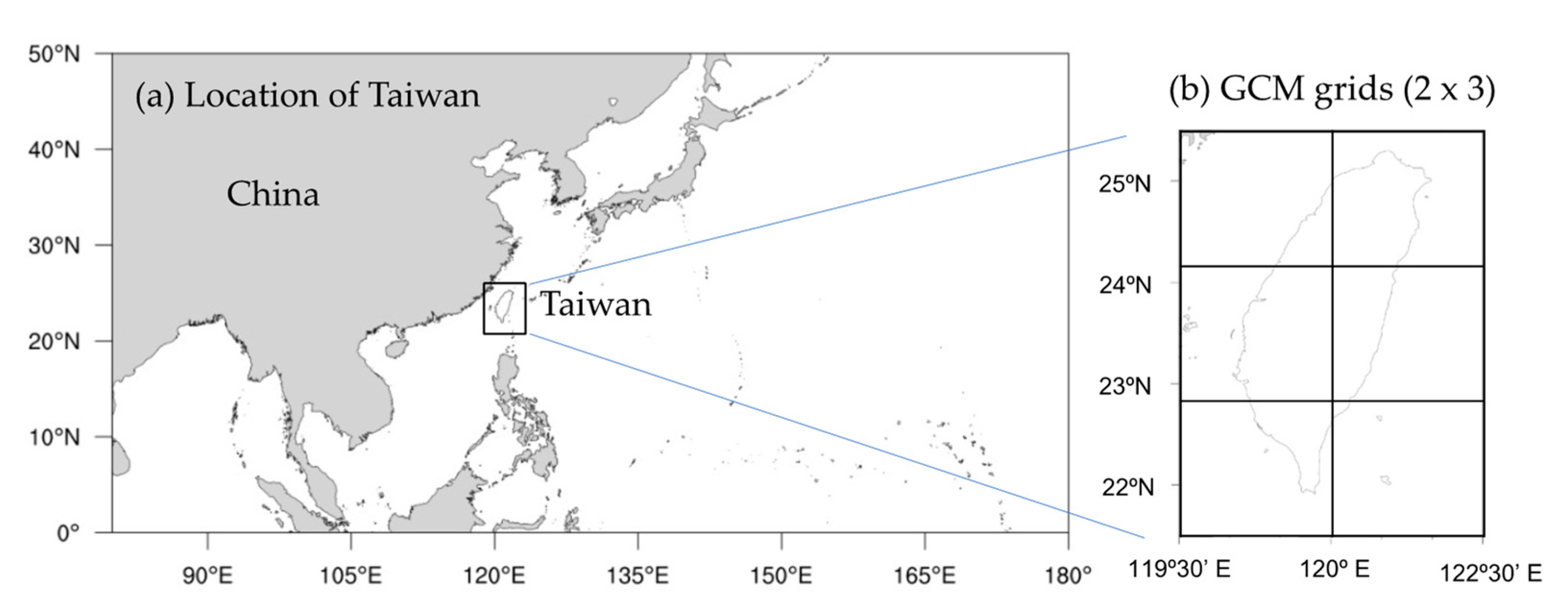
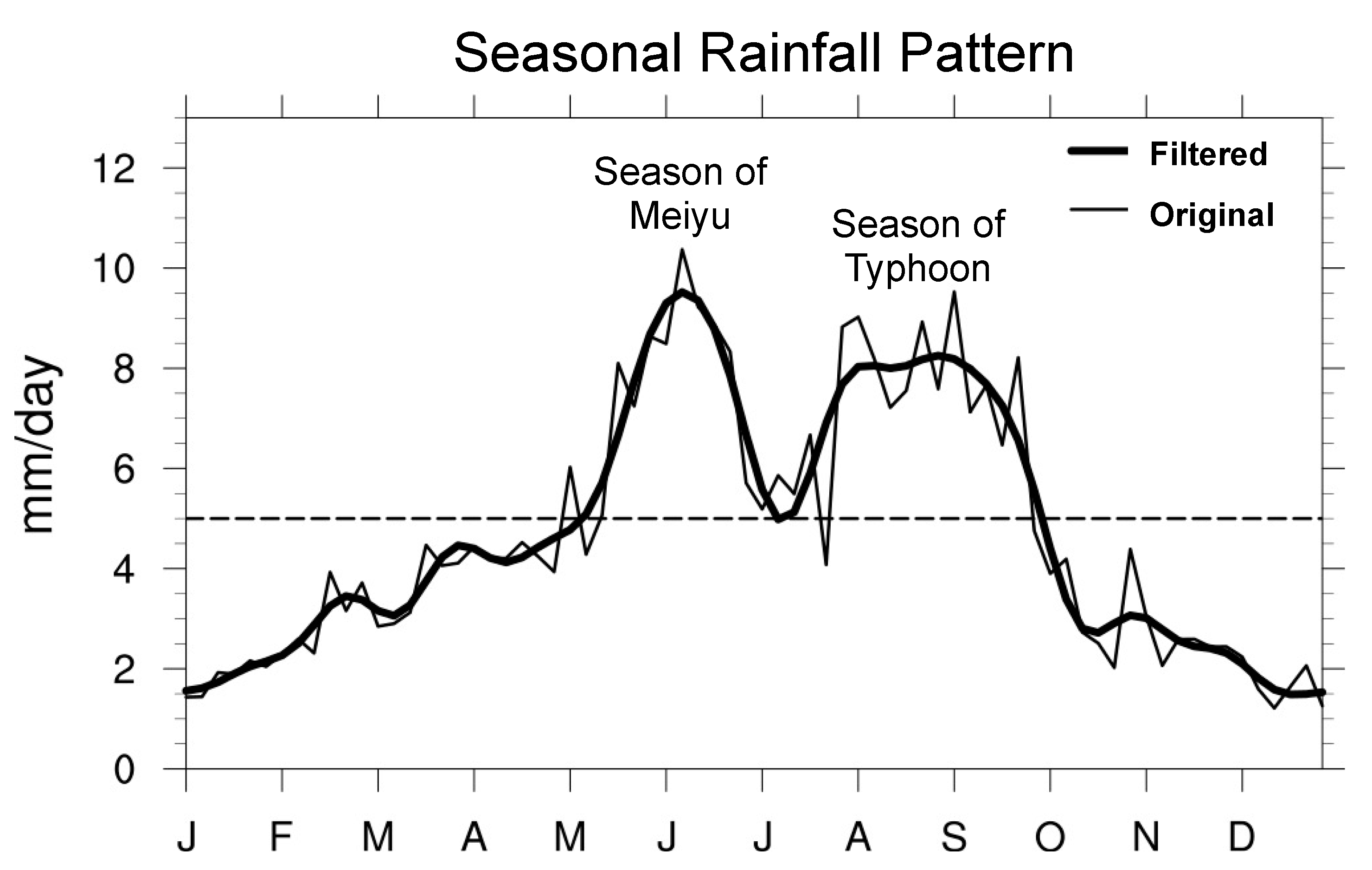
This method evaluates the rainfall performance of GCMs in the baseline period. The observation data are selected grid data with similar time and space resolutions; the area is shown in Figure 1a. After the model is processed into the same format as the observation data, Fourier analysis is performed to filter out high-frequency signals (especially during the Meiyu and typhoon seasons) (Wang and Lin, 2002) [14] (Figure 2).
This study uses the method of Reichler and Kim (2008) [13] to target the seasonal cycle of rainfall in the GCM model, using the performance index as the evaluation standard. The formula is shown below.
where n = total grid points; m = model; = weight index of individual grid points; = model simulation value (average of the selected period); = observed value (average of the selected period); and = variance of observation data.
Formula (1) was used to calculate the difference between the simulated grid and the observation data in all GCMs where the total number of grids (n) = 6 (Figure 1b), the number of models (m) = 33, and = 1. Formula (2) was used to standardize the variance, calculate the scores of all GCMs, and then sort them. The list of 33 GCMs and the ranking results of the performance index are shown in Table 1.
According to the GCMs performance ranking, the top five GCMs, CanESM2, CMCC-CM, MIROC5, MPI-ESM-LR, and HadGEM2-ES, were selected for follow-up analysis and discussion.
2.3. Study Area and Observation Data
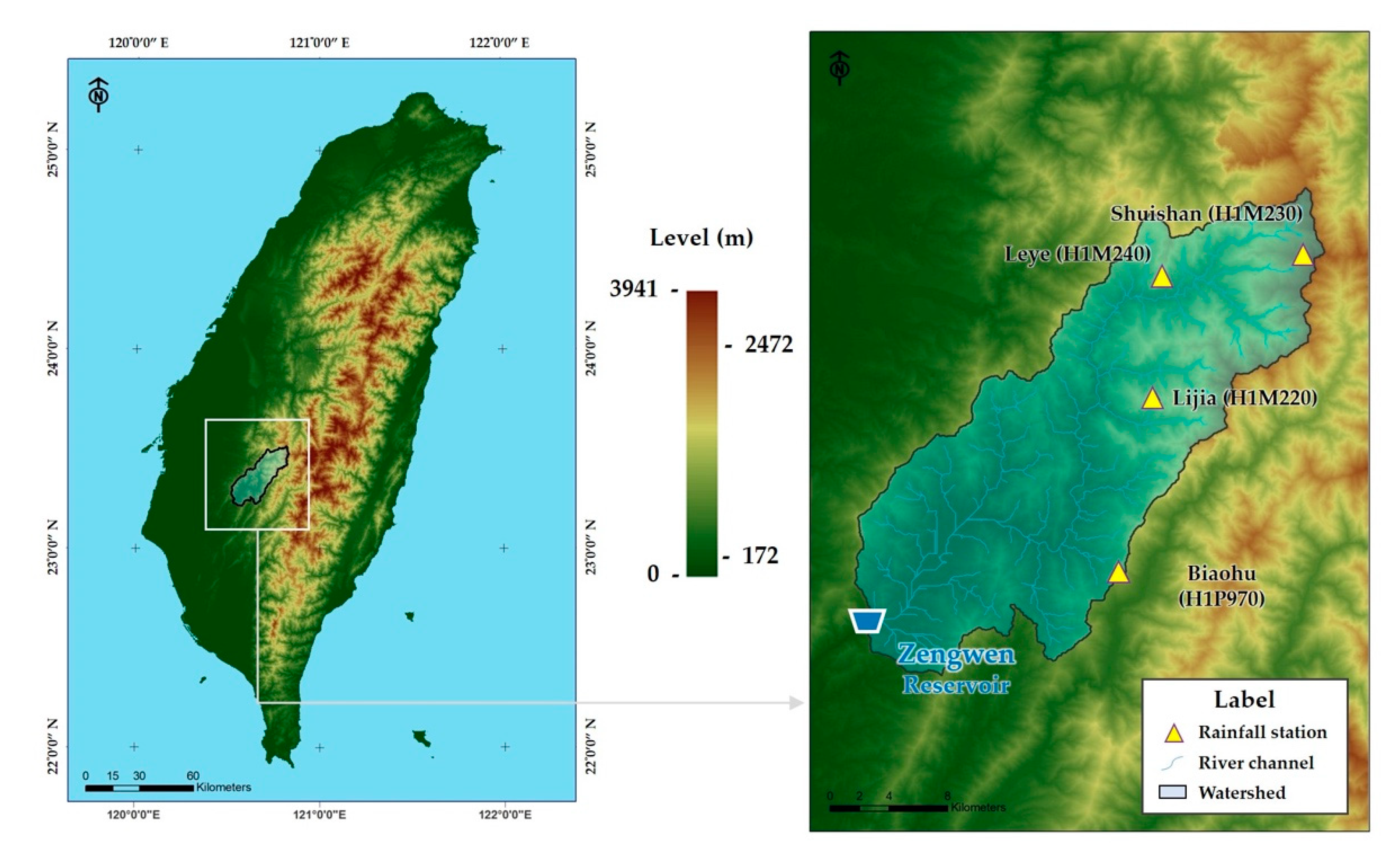
In this study, an important water resource facility in southern Taiwan, the watershed of the Zengwen Reservoir, was selected as the analysis objective. The daily rainfall data observed by the rainfall station (hereinafter station data) are applied in this study.
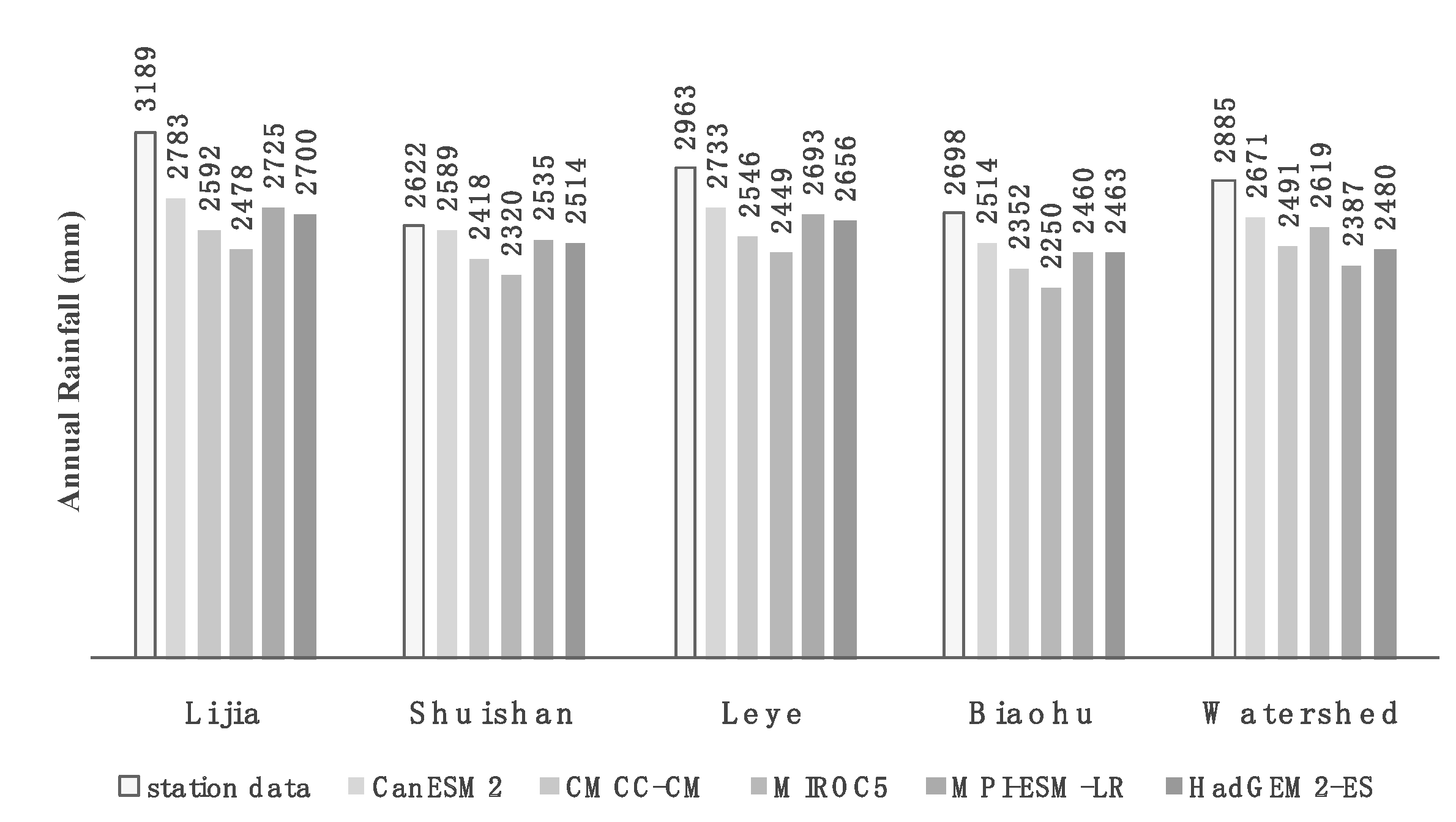
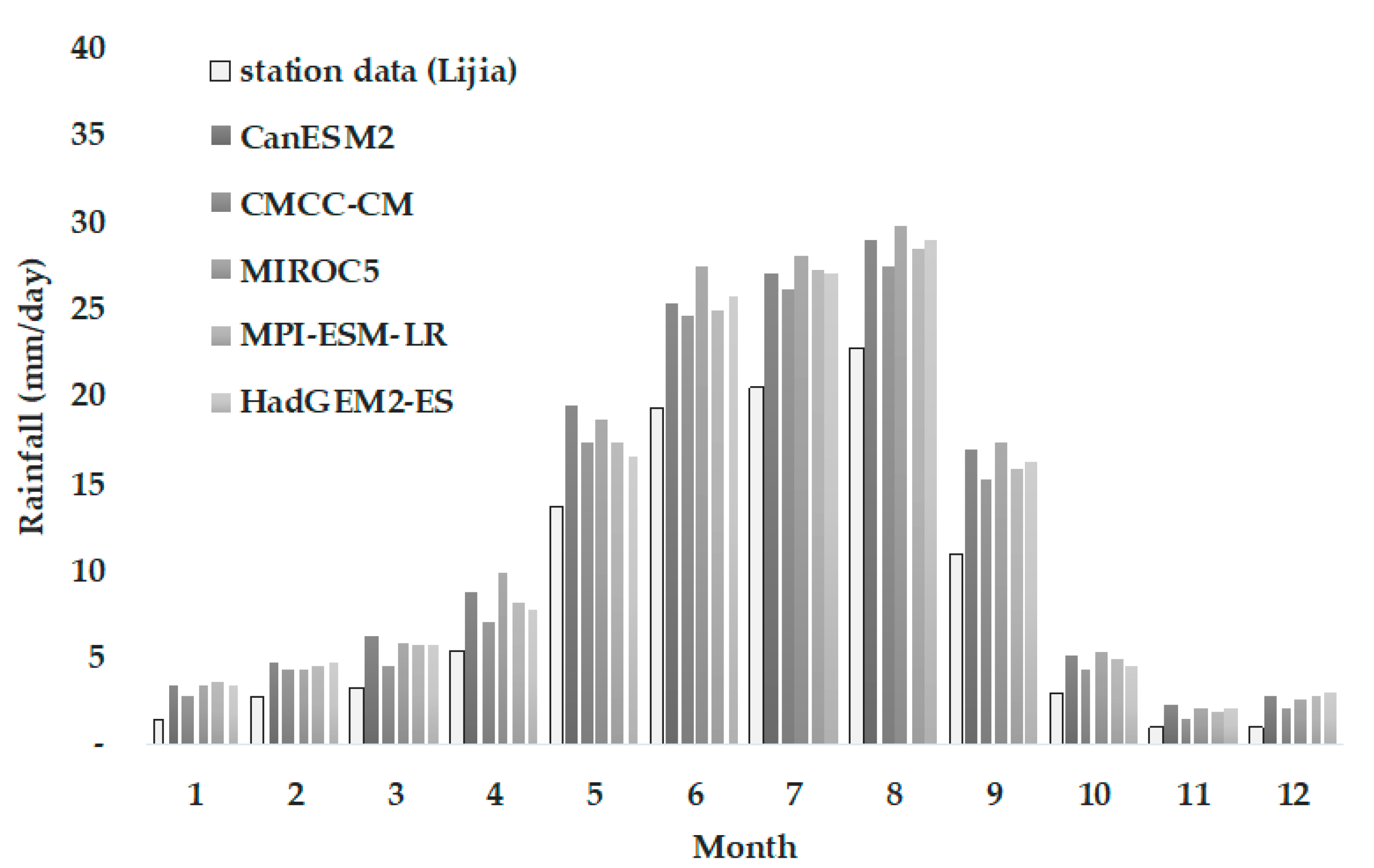
Four rainfall stations in the watershed, namely, Lijia (H1M220), Shuishan (H1M230), Leye (H1M240), and Biaohu (H1P970), were selected. All had valid records for 30 years (1976–2005). Figure 3 shows the geographical location of the watershed and rainfall stations of the Zengwen Reservoir.
The average annual rainfall (1976–2005) of the selected four rainfall stations is about 2622–3189 mm, and the average rainfall in the watershed is about 2910 mm (Thiessen’s Polygon Method was applied). The rainfall is concentrated in the wet season (May to October) and accounts for about 85% of the total annual rainfall, and the dry season (November to April) accounts for 15% of the rainfall. Table 2 shows the basic data of the rainfall stations in the watershed of the Zengwen Reservoir.
2.4. Hydrological Model
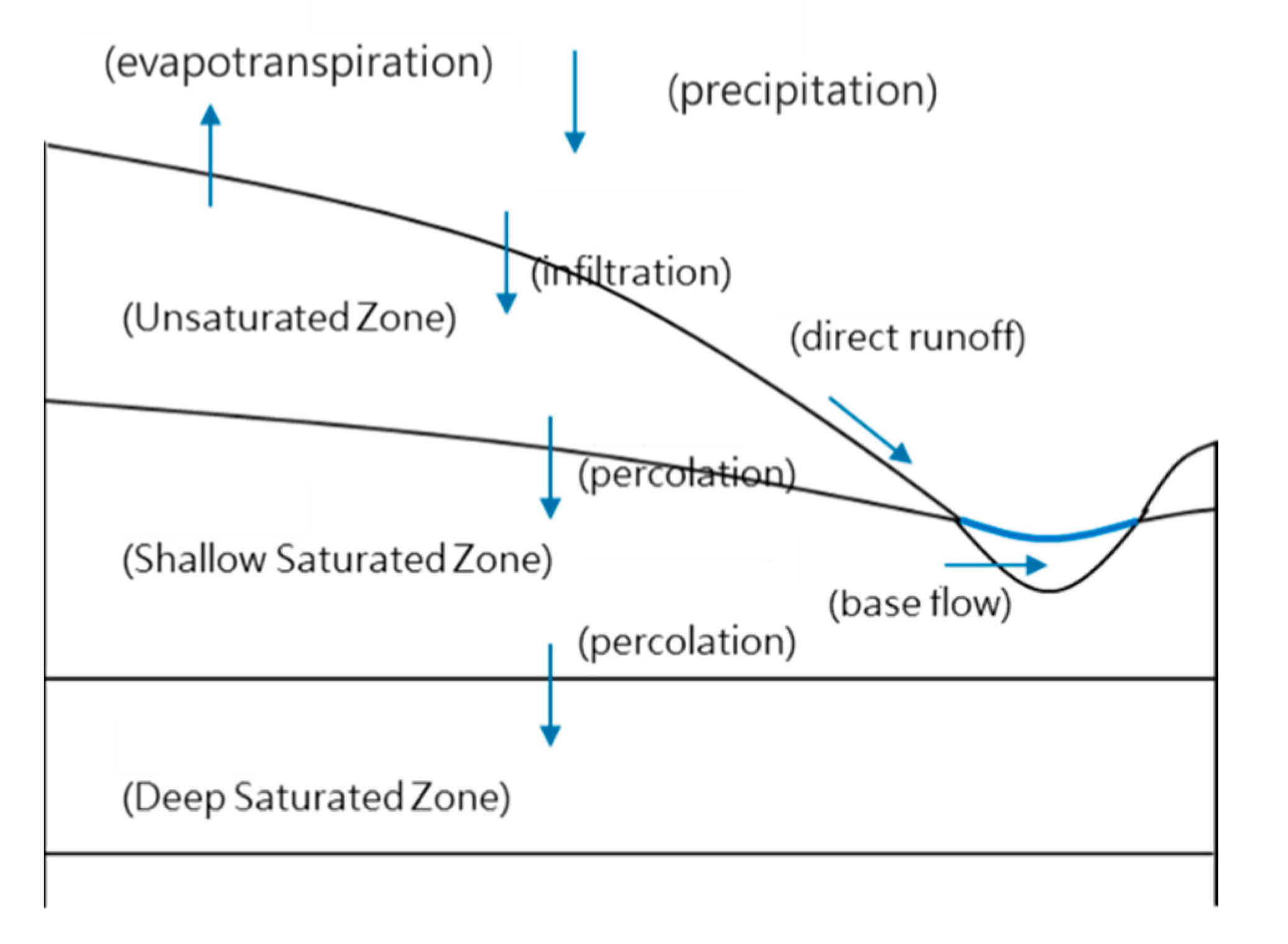
To evaluate the bias of the watershed runoff simulation, the Generalized Watershed Loading Function (GWLF) (Haith et al., 1992) [15] was used in this study. The input of GWLF water balance mechanism is mainly from precipitation. When the rainfall reaches the ground, part of the rainfall goes underground through the infiltration mechanism, and some forms direct runoff. The infiltration rainfall supplements the water of the unsaturated zone. When the soil moisture in the unsaturated zone reaches the field capacity, the excess water will pass through the percolation mechanism to the shallow saturated zone, and finally the shallow saturated zone will produce base flow. The stream flow is the sum of the direct runoff and base flow. The concept of the water balance model is illustrated in Figure 4.
The parameters required by the GWLF include the area and the land use (represented by the CN value) of the watershed which is shown as Table 3.
3. Two-Stage Bias Correction Method
Comparing the rainfall data of the four rainfall stations with five selected GCMs in the baseline (1976–2005) period, the rainfall data of five selected GCMs are underestimated compared to the four stations, with an average underestimation of about 12% and the largest gap being more than 20%. The average rainfall of the watershed calculated with grid data (Thiessen’s Polygon Method) is also underestimated, with an average underestimation of about 13% (Table 4). The annual rainfall comparison between the station data and the GCM data is shown in Figure 5.
In order to correct the rainfall gap between GCM data and station data, this study proposes a two-stage bias correction method. A quantile mapping empirical cumulative distribution function (ECDF) procedure is the basis of this method as the first stage. In addition, the wet-day threshold of the GCM data is optimized to fit the probability of precipitation of the station data to achieve an effective rainfall bias correction result as the second stage. Detailed descriptions are provided below.
3.1. Quantile Mapping Bias Correction Method
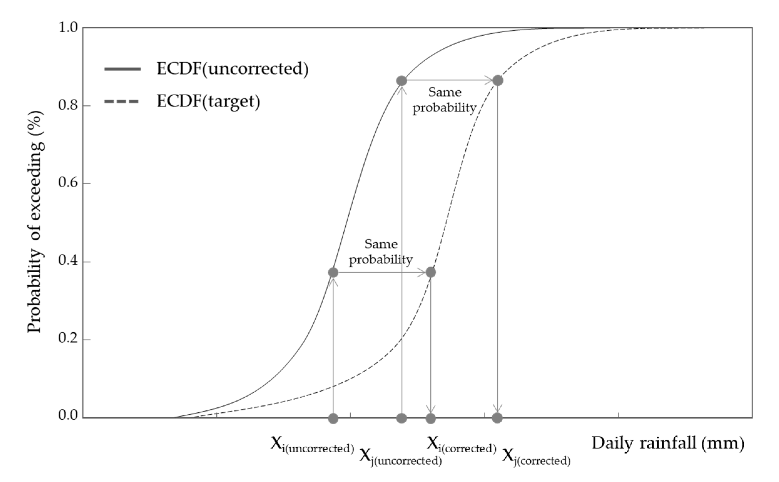
In view of the gap between the GCM data and station data, this study refers to the quantile mapping empirical cumulative distribution function (ECDF) method used in bias correction of a climate model and adjusts the ECDF curve of the GCM data to conform to the ECDF curve of the station data.
First, the ECDF curve of the daily rainfall data (wet days) of the GCM baseline period and the ECDF curve of the station daily rainfall data (wet days) are calculated, and then the GCM baseline period daily rainfall events are corrected according to the ECDF value corresponding to the station daily rainfall data. The schematic diagram of bias correction is shown in Figure 6.
Taking into account the differences in the rainfall amount and patterns of each month, this study uses wet days from individual months to establish the ECDF curves, and the ECDF curves from stations and GCMs differ. The probability of exceeding on a wet days is calculated using the Weibull method. The formula is as follows:
where m is the ranking of wet days from small to large, and n is the total number of wet days.
3.2. Wet-Day Threshold Optimization
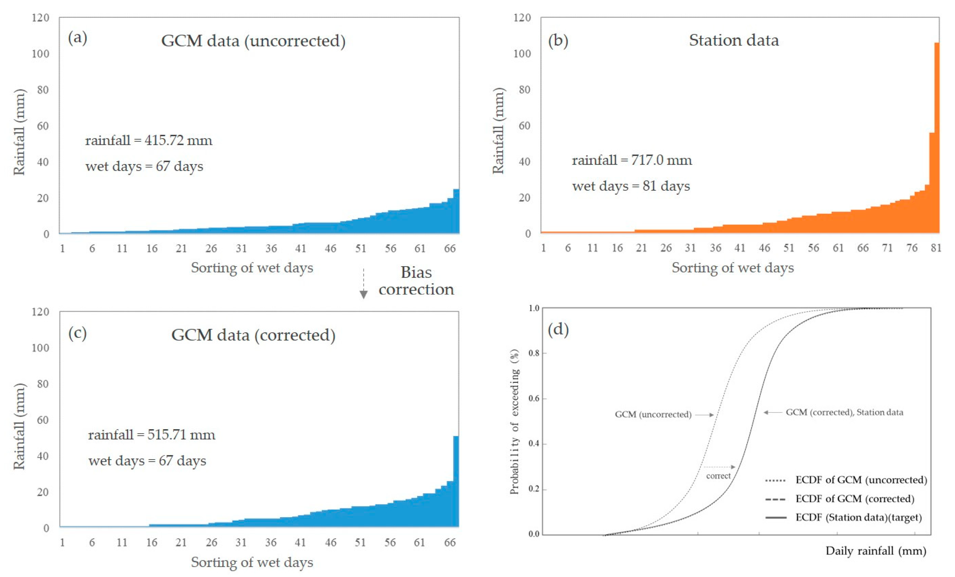
However, although the correction method can make the two sets of data consistent with the rainfall of the same ECDF value, there is still a gap in comparison to the total rainfall. This study found that the gap is caused by the different numbers of wet days in the two groups of data. Because the input of the bias correction is wet-day data, then even though the wet days are corrected by the quantile mapping method, the monthly and annual rainfall of the corrected GCM data will not fit the station data due to the difference in the numbers of wet days.
For example, in Figure 7, Case 1a represents the original GCM grid daily data (not corrected yet) (Figure 7a), Case 1b represents the GCM gridded daily data that has been corrected by the traditional quantile mapping method (Figure 7b), and Case 2 represents the station data (Target) (Figure 7c). Although the ECDF curve of Case 1a has been corrected to fit the target Case 2 (Figure 7a is corrected to Figure 7b), the total rainfall amounts of the corrected result Case 1b and the target value Case 2 are still different. Therefore, it is necessary to redefine the wet-day determination method for GCM data if consistency in the total rainfall amount is a consideration.
Although there is no specific method for determining wet days, it is common to define the threshold of a wet day for specific purposes to collate meteorological data. WMO (Karl et al., 1999 [16], Peterson et al., 2001 [17]) uses the wet-day threshold of 1.0 mm as the basis for calculating consecutive wet days and consecutive dry days, and the agricultural department in Taiwan uses the threshold value of 0.6 mm as the basis for calculating the number of consecutive dry days.
The above problem (the difference in total rainfall between the two groups of data) is caused by the inconsistency of wet days. Therefore, this study attempts to use the probability of precipitation of the station data as the objective function and adjusts the wet-day threshold value of the GCM data such that the probability of the GCM data fits the station data.
However, the mechanisms of rainfall of the two systems are not identical. The rainfall in the GCM data is the spatial average of the rainfall in the entire grid, not the actual measured value. Thus, extremely small amounts rainfall (such as daily rainfall = 0.0001 mm) may occur, and the probability of precipitation is therefore much higher than indicated by the station data. In addition, the rainfall in the station data is measured by an instrument, and different instruments may have different minimum values.
Based on the assumption that the probability of precipitation of the GCM data under the same location should be equal to the probability of the station data, this study establishes the wet-day threshold optimization mechanism of the GCM data corresponding to the station data to filter out the extra small rainfall events of the GCM data and make the probabilities of rainfall identical.
The calculation process of the optimized wet-day threshold first calculates the probability of precipitation of the station data, and then optimizes the wet-day threshold value under the same probability of the GCM data to achieve equality in the rainfall probabilities of the GCM data and the station data. Then, the optimized value of the wet-day threshold is used as an input for bias correction. The results of the bias correction will be similar to the station data in both the average daily rainfall and the number of rainfall days in each month.
4. Analysis and Discussion
In this study, a two-stage bias correction method was established for GCM data of the Zengwen Reservoir watershed. The key issue is that precipitation threshold will affect the result of the bias correction. Therefore, the different methods for different wet-day thresholds were applied to the second stage of bias correction.
4.1. Analysis with Different Wet-Day Thresholds
Rainfall station Lijia (H1M220) of the Southern Region Water Resources office was selected as the target, and the bias correction results of three different wet-day thresholds were compared, as follows: No-Threshold method (wet-day threshold = 0 mm); Fixed-Threshold method (threshold = 1 mm); and Optimized-Threshold method (GCM data wet-day threshold optimized by the probability of precipitation of the station data). The studied period was 1976–2005. The results were compared in three hydrological amounts, such as average daily rainfall, probability of precipitation, and annual runoff, to reveal the bias of different wet-day thresholds.
4.1.1. Comparison to Averaged Daily Rainfall
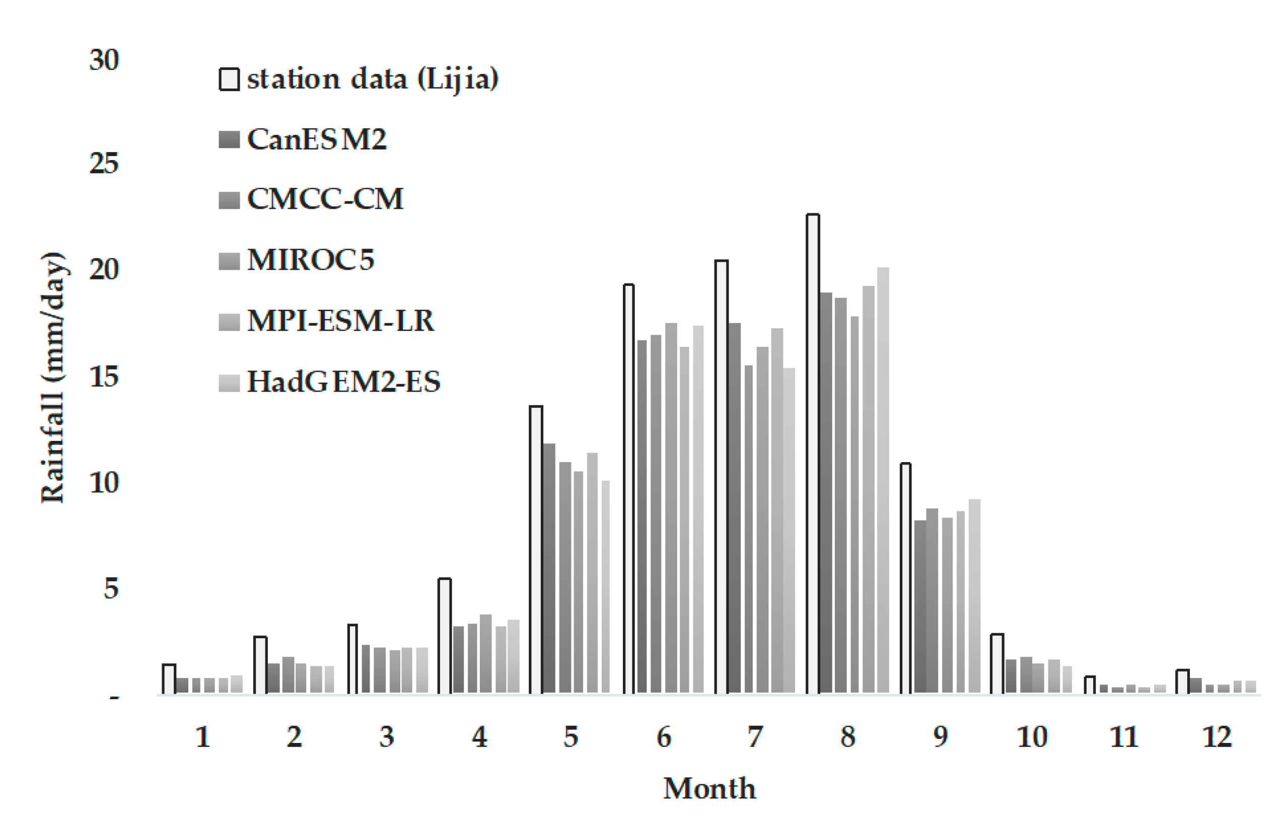
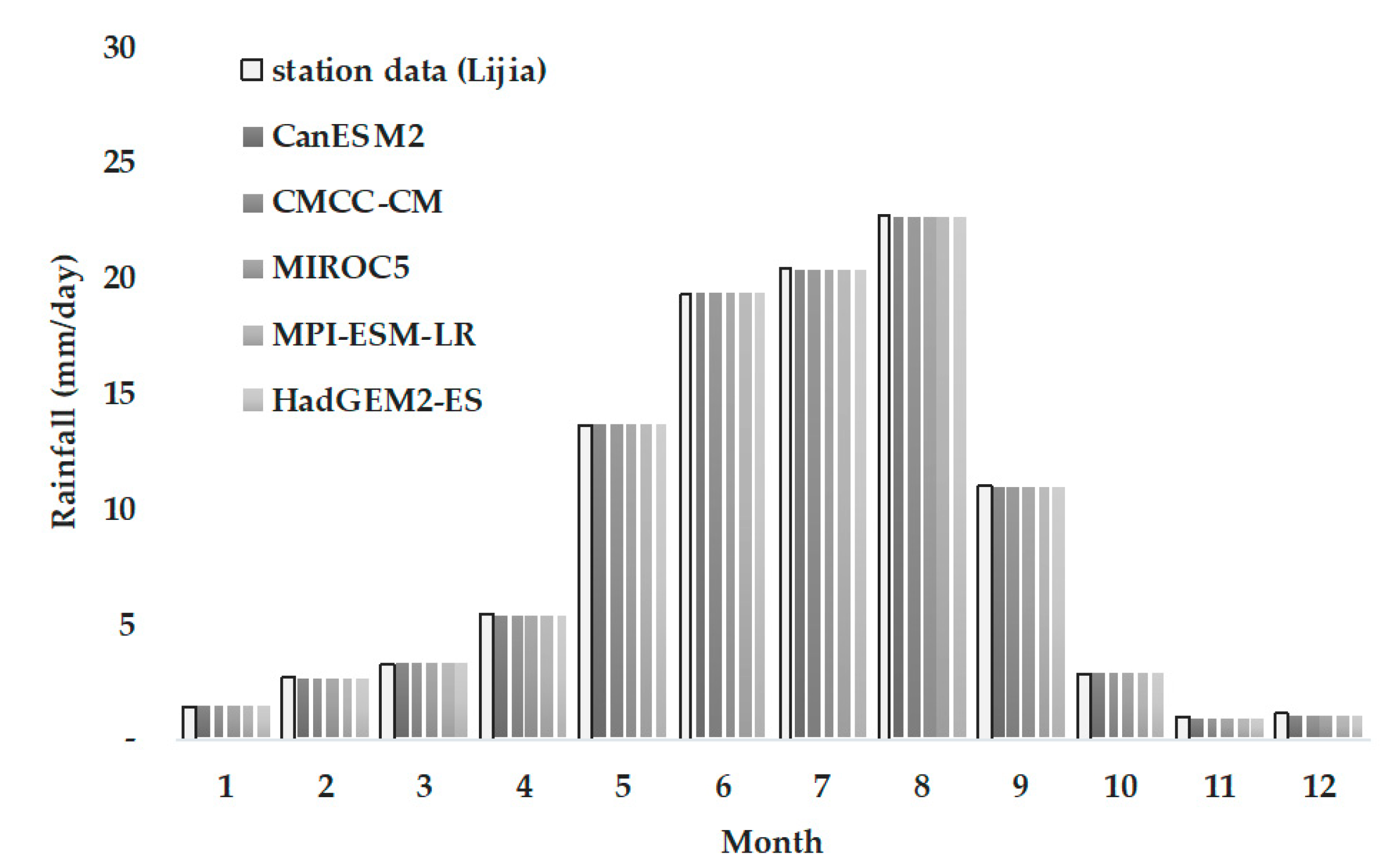
For the bias correction results of the No-Threshold method, the daily rainfall of the five GCMs was significantly higher than the station data (Figure 8). The results of the Fixed-Threshold method were lower than the station data (Figure 9), and the Optimized-Threshold method produced results basically identical to the station data (Figure 10).
4.1.2. Comparison to Probability of Precipitation
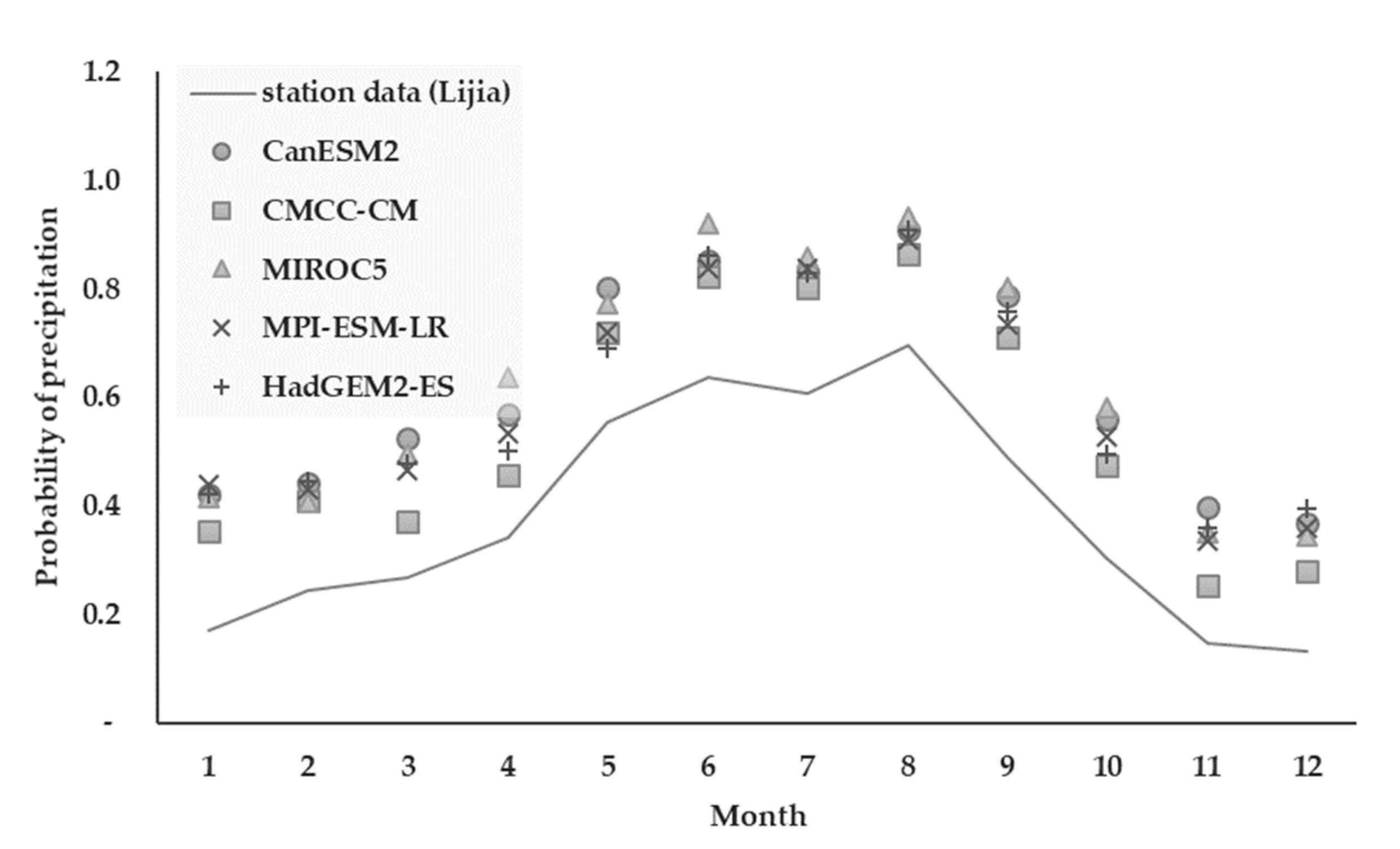
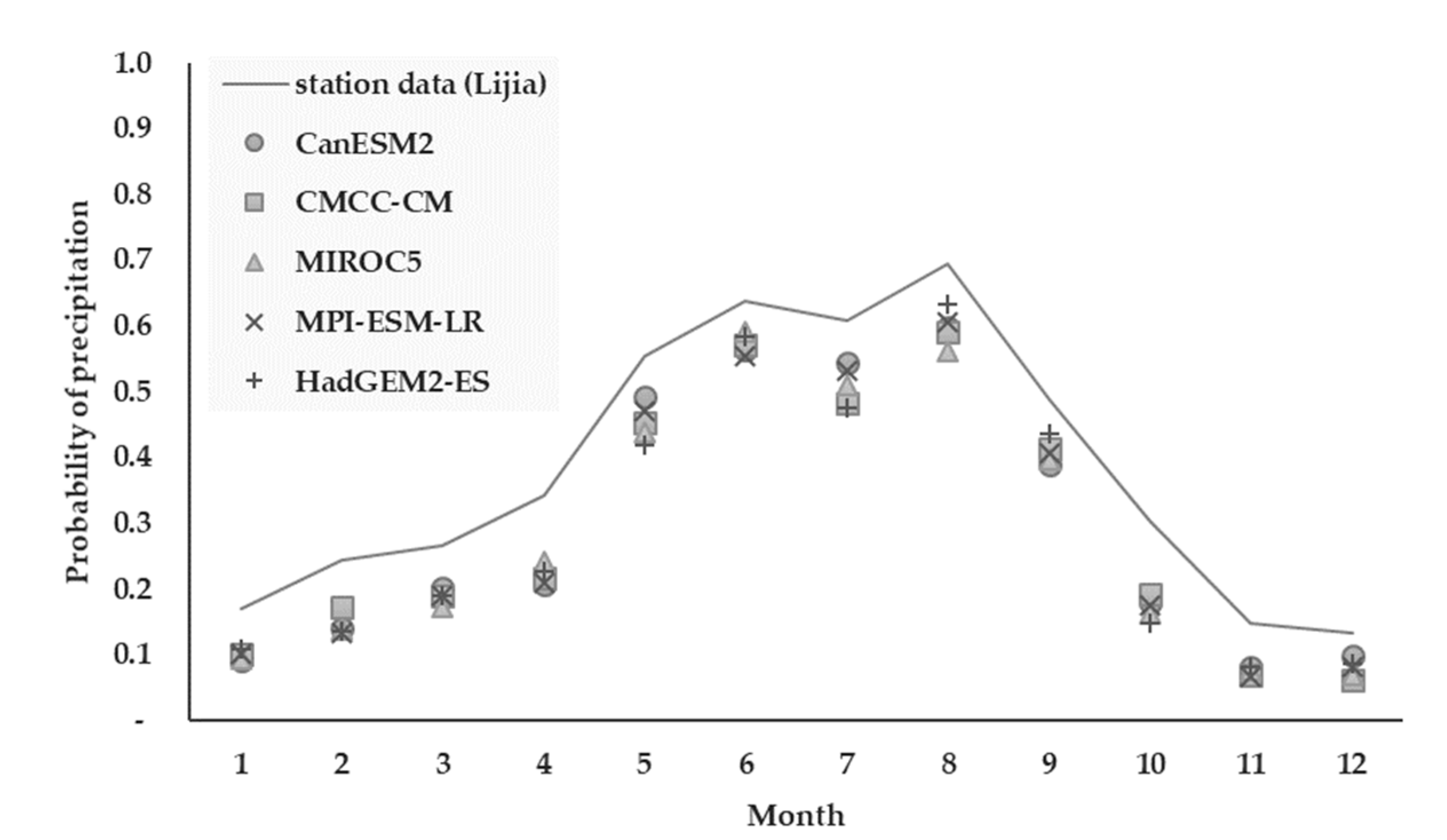
This study also presents the difference in the probability of precipitation (number of wet days/total number of days) in the results of the three correction methods. With the No-Threshold method, the probability of the GCM data was significantly higher than the station data, so the bias correction results were overestimated (Figure 11). With the Fixed-Threshold method, it was generally lower than the station data; therefore, the correction results were underestimated (Figure 12). With the Optimized-Threshold method, the rainfall probabilities of the two groups of data were identical, so the correction results were basically the same (Figure 13).
4.1.3. Comparison to Annual Average Runoff of the Watershed
Three different kind of rainfall data (station data, original GCM data, and corrected GCM data) were used to simulate the flow and water resources amount in the watershed of the Zengwen Reservoir. With the original GCM data used as the input of GWLF, the results of the five GCMs show that the annual average flow depth of the watershed is 1655–1860 mm. The result of the No-Threshold method is 3155–3651 mm, that of the Fixed-Threshold method is 1609–1673 mm, and that of the Optimized-Threshold method is 2217–2202 mm (Table 5).
For the annual average flow volume of the catchment area (maximum available water resources), the result of the original GCM data is 796–894 million m3/year, that of the No-Threshold method is 1.518–1.756 billion m3/year, that of the Fixed-Threshold method is 774–805 million m3/year, and that of the Optimized-Threshold method is 1.023–1.059 billion m3/year (Table 6).
Comparing the above results, the flow simulation results of the original GCM data underestimate the water resources by nearly 150 million m3/year. The No-Threshold method overestimates them by about 640 million m3/year; the Fixed-Threshold method, by about −220 million m3/year; and the Optimized-Threshold method, by only about 35 million m3/year (Table 7).
4.2. Discussion
The GCM data were inconsistent with the station data before they were corrected and underestimated compared with the station data. Based on the quantile mapping method, the wet-day threshold determines the fitness of the correction result between the GCM data and the station data. Whether a wet-day threshold of 0 or 1 mm is used, it cannot effectively match the rainfall characteristics of the station data. Only by considering the probability of precipitation of the station data (Optimized-Threshold method) can an effective correction of the bias of GCM data be achieved.
However, during the research process, it was also found that this method still has limitations. For example, the probability of precipitation of GCM data can only be reduced and not increased. The analysis of the five GCMs shows that the probability of precipitation is much higher than the station data, for which two-stage bias correction still works. However, if the probability of the GCM data is already lower than the station data, the method of optimizing the wet-day threshold cannot be used to make the probabilities of rainfall equal because the rainfall event cannot be created to increase the probability of precipitation.
In addition, this study assumes that the probability of precipitation of the station data under the same location is equal to that of the GCM data. A numerical method is used to make the two sets of data equal. Although the correction result can be achieved, it does change the number of physical rainfall events in the GCM. The number of wet days in the GCM data is reduced, and some rainfall events are missing, because such rainfall events are below the threshold and calculated as dry days.
Whether this approach has perfect physical significance will require further research to determine. However, in terms of a water resources system, the rainfall that is filtered out is a relatively small value. Whether it is filtered out or not does not affect the overall catchment flow or the performance of the water resources system, and its advantages make it easier to analyze and compare GCM data and station data. It is also an alternative method to deal with climate change data.
5. Conclusions
Even though the statistical downscaling skill has improved and refined GCMs for climate change impact assessment from monthly data to daily data, there is still bias between GCM data and station data. This gridded data to point data issue will affect the result of water resources amount assessment.
The quantile mapping bias correction method is usually adopted to reduce the bias between GCM data and station data; however, there is still a gap after bias correction which is caused by the different wet days in these two sets of data.
This study proposed the two-stage bias correction method to convert GCM gridded data to station data which optimized the wet-day threshold value of the GCM data to achieve equality in the rainfall probabilities of the GCM data and the station data. After two-stage bias correction, the GCM data will fit to the station data in both the average daily rainfall and the number of rainfall days in each month.
Because of the bias between GCM data and station data, there will be quite an amount of bias after applying data to the watershed runoff simulation. In the case of the Zengwen reservoir inflow simulation, with regard to the result of applying original GCM data as input, there is a bias of about 154 million m3/year, which is an about 15% bias compared to the result with the input of station data. Applying the data with a two-stage bias correction to the Zengwen reservoir inflow simulation, the bias was reduced to 3%. This result indicates that the GCM data can be directly applied to water resources amount evaluation after two-stage bias correction; however, the bias still needs to be counted to establish the uncertainty of climate change assessment.
To reveal the effectiveness of two-stage bias correction and the bias after converting gridded data to station data, the GCM selection method was used in this study to reduce the running cases. The result of the GCM performance ranking can also apply to other studies that uses CMIP5 GCMs daily data in Taiwan.
Author Contributions
Conceptualization, T.-Y.T., T.-M.L. and K.-S.C.; methodology, T.-Y.T., T.-M.L. and K.-S.C.; formal analysis, T.-Y.T.; investigation, T.-Y.T.; resources, Y.-S.T.; data curation, Y.-S.T.; writing—original draft preparation, T.-Y.T.; writing—review and editing, T.-M.L.; supervision, K.-S.C. All authors have read and agreed to the published version of the manuscript.
Funding
This research was funded by Ministry of Science and Technology, Taiwan. Project number: MOST 108-2621-M-865-001 and MOST 109-2621-M-865-001.
Institutional Review Board Statement
Not applicable.
Informed Consent Statement
Not applicable.
Data Availability Statement
The study did not report any data.
Acknowledgments
This research was supported by the Ministry of Science and Technology (MOST) “Taiwan Climate Change Projection Information and Adaptation Knowledge Platform” (MOST 108-2621-M-865-001) and (MOST 109-2621-M-865-001). Special thanks to Chao-Tzuen Cheng, Jun-Jih Liou, and Shih-Yao Lin from the National Science and Technology Center for Disaster Reduction for the technical guidance and support.
Conflicts of Interest
The authors declare no conflict of interest.
References
- Water Resources Agency. Strengthening Water Supply System Adaptive Capacity to Climate Change in Southern Region; Water Resources Agency: Taipei, Taiwan, 2011. (In Chinese) [Google Scholar]
- Jones, P.; Harpham, C.; Kilsby, C.; Glenis, V.; Burton, A. UK Climate Projections Science Report: Projections of Future Daily Climate for the UK from the Weather Generator, Project Report; UK Climate Projections; Met Office: Exeter, UK, 2010. [Google Scholar]
- Tung, Y.S.; Chen, C.T.; Liu, J.J.; Chen, Y.M. Daily Statistics Downscaling for CMIP5 AGCM: Validation and Application; NCDR 107-T19; National Science and Technology Center for Disaster Reduction: New Taipei Cty, Taiwan, 2018. (In Chinese) [Google Scholar]
- Liu, H.W.; Lin, S.L.; Chen, C.T.; Tung, Y.S.; Chen, Y.M. Key Indicators of Climate Change in Taiwan; National Science and Technology Center for Disaster Reduction: New Taipei city, Taiwan, 2019. (In Chinese) [Google Scholar]
- Li, Y.C.; Wang, C.C.; Weng, S.P.; Chen, C.T. Future Projections of Meteorological Drought Characteristics in Taiwan. Atmos. Sci. 2019, 47, 66–91. [Google Scholar]
- Huang, Y.W.; Liu, H.W. Assessment of the impact of rainfall on grapes under climate change-Taking Changhua County as an example. Newsl. Taiwan Clim. Chang. Proj. Inf. Adapt. Knowl. Platf. 2019, 32. Available online: https://tccip.ncdr.nat.gov.tw/km_newsletter_one.aspx?nid=20191005114602 (accessed on 25 May 2021). (In Chinese).
- Tung, Y.S.; Liu, T.M.; Chang, C.W.; Sun, S.; Lin, S.Y.; Huang, Y.C.; Lee, H.L. Questions and Answers on Statistical Downscaling Daily Data; National Science and Technology Center for Disaster Reduction: New Taipei City, Taiwan, 2019. (In Chinese) [Google Scholar]
- Ines, A.V.M.; Hansen, J.W. Bias correction of daily GCM rainfall for crop simulation studies. Agric. For. Meteorol. 2006, 138, 44–53. [Google Scholar] [CrossRef] [Green Version]
- Johnson, F.; Sharma, A. Accounting for interannual variability: A comparison of options for water resources climate change impact assessments. Water Resour. Res. 2011, 47, W04508. [Google Scholar] [CrossRef]
- Su, Y.F.; Cheng, C.T.; Liou, J.J.; Chen, Y.M.; Kitoh, A. Bias correction of MRI-WRF dynamic downscaling datasets. Terr. Atmos. Ocean. Sci. 2016, 27, 649–657. [Google Scholar] [CrossRef] [Green Version]
- Intergovernmental Panel on Climate Change (IPCC). Summary for Policymakers. In Climate Change 2013: The Physical Science Basis. Contribution of Working Group I to the Fifth Assessment Report of the Intergovernmental Panel on Climate Change; Cambridge University Press: Cambridge, UK; New York, NY, USA, 2013. [Google Scholar]
- Tung, Y.S.; Wang, S.Y.; Chu, J.L.; Wu, C.H.; Chen, Y.M.; Cheng, C.T.; Lin, L.Y. Projected increase of the East Asian summer monsoon (Meiyu) in Taiwan by climate models with variable performance. Meteorol. Appl. 2020, 27, e1886. [Google Scholar] [CrossRef] [Green Version]
- Reichler, T.; Kim, J. How well do coupled models simulate today’s climate? Bull. Am. Meteor. Soc. 2008, 89, 303–311. [Google Scholar] [CrossRef]
- Wang, B.; Lin, H. Rainy Season of the Asian–Pacific Summer Monsoon. J. Clim. 2002, 15, 386–398. [Google Scholar] [CrossRef] [Green Version]
- Haith, D.A.; Mandel, R.; Wu, R.S. GWLF, Generalized Watershed Loading Functions, Version 2.0, User’s Manual; Department of Agricultural & Biological Engineering, Cornell University: Ithaca, NY, USA, 1992. [Google Scholar]
- Karl, T.R.; Nicholls, N.; Ghazi, A. CLIVAR/GCOS/WMO workshop on indices and indicators for climate extremes: Workshop summary. Clim. Chang. 1999, 42, 3–7. [Google Scholar] [CrossRef]
- Peterson, T.C.; Folland, C.; Gruza, G.; Hogg, W.; Mokssit, A.; Plummer, N. Report on the Activities of the Working Group on Climate Change Detection and Related Rapporteurs 1998–2001; WMO/TD-No. 1071; WCDMP-No. 47; World Meteorological Organization: Geneva, Switzerland, 2001. [Google Scholar]
Figure 1.
Evaluation area of GCM performance. (a) Location of Taiwan in east Asia; (b) Sketch diagram of 6 points over Taiwan in GCM which were adopted to calculate performance index.
Figure 1.
Evaluation area of GCM performance. (a) Location of Taiwan in east Asia; (b) Sketch diagram of 6 points over Taiwan in GCM which were adopted to calculate performance index.

Figure 2.
Schematic diagram of seasonal rainfall pattern and data filter (made by this study).

Figure 3.
Geographical location of the watershed and rainfall stations of Zengwen Reservoir (made by this study).
Figure 3.
Geographical location of the watershed and rainfall stations of Zengwen Reservoir (made by this study).

Figure 4.
Concept of GWLF water balance model (made by this study).

Figure 5.
Annual rainfall of the station data and GCM data.

Figure 6.
Schematic diagram of quantile mapping bias correction.

Figure 7.
Example of quantile mapping bias correction and the bias of wet days. (a) demonstrates the sample of uncorrected GCM data in a certain month, (b) demonstrates the sample of station data in the same month, (c) demonstrates the sample of corrected GCM data in the same month, and (d) shows the correction process of ECDF of sample data. The bias correction corrects GCM data from (a–c), by considering the ECDF characteristic of station data (b). The bias correction makes the ECDF of GCM data corrected to match the ECDF of station data (d), therefore correcting the rainfall value, but the number of wet days is still unchanged.

Figure 8.
Bias correction result in rainfall of the No-Threshold method.

Figure 9.
Bias correction result in rainfall of the Fixed-Threshold method.

Figure 10.
Bias correction result in rainfall of the Optimized-Threshold method.

Figure 11.
Bias correction result in probability of precipitation of the No-Threshold method.

Figure 12.
Bias correction result in probability of precipitation of the Fixed-Threshold method.

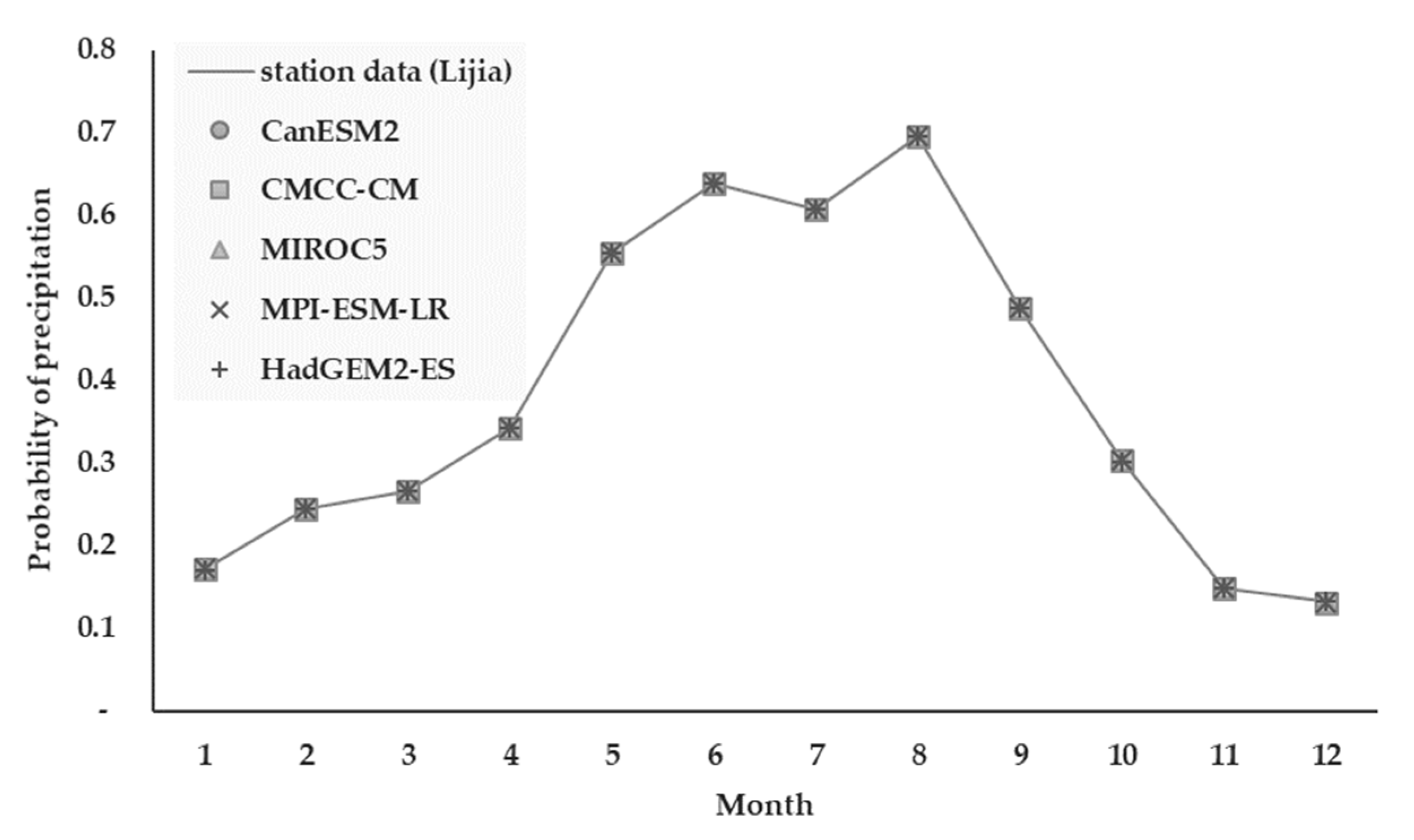
Figure 13.
Bias correction result in probability of precipitation of the Optimized-Threshold method.
Figure 13.
Bias correction result in probability of precipitation of the Optimized-Threshold method.


Table 1.
The list of 33 GCMs (refer to PCMDI website (https://pcmdi.llnl.gov/mips/cmip5/availability.html, accessed on 24 May 2021)) and the results of performance ranking (ranking was made by this study).
Table 1.
The list of 33 GCMs (refer to PCMDI website (https://pcmdi.llnl.gov/mips/cmip5/availability.html, accessed on 24 May 2021)) and the results of performance ranking (ranking was made by this study).
| Model Name | GCM Center | Description | Ranking |
|---|---|---|---|
| ACCESS1-0 | CSIRO-BOM | Australian Community Climate and Earth System Simulator 1.0 | 13 |
| ACCESS1-3 | Australian Community Climate and Earth System Simulator 1.3 | 30 | |
| bcc-csm1-1 | BCC | Beijing Climate Center Climate System Model version 1.1, China | 22 |
| bcc-csm1-1m | Beijing Climate Center Climate System Model version 1.1, China, high resolution | 9 | |
| BNU-ESM | BNU | College of Global Change and Earth System Science, China, Beijing Normal University Earth System Model | 8 |
| CanESM2 | CCCMA | Canadian Earth System Model version 2 | 1 |
| CCSM4 | NCAR | NCAR Community Climate System Model version 4.0 | 18 |
| CESM1-BGC | NCAR | NCAR Community Earth System Model version 1 with carbon cycle | 27 |
| CESM1-CAM5 | Coupled simulations from CESM1 using the atmosphere model of Community Atmosphere Model version 5 | 19 | |
| CMCC-CESM | CMCC | Centro Euro-Mediterraneo per I Cambiamenti Climatici (CMCC) Carbon Earth System Model | 26 |
| CMCC-CM | Centro Euro-Mediterraneo per I Cambiamenti Climatici Climate Model | 3 | |
| CNRM-CM5 | CNRM-CERFACS | Centre National de Recherches Meteorologiques (CNRM) Earth System Model version 5, France | 15 |
| CSIRO-Mk3-6-0 | CSIRO-QCCCE | CSIRO Atmospheric Research, Australia, Mk3.6 Model | 23 |
| EC-EARTH | ICHEC | Canadian Earth System Model version 2 | 29 |
| FGOALS-g2 | LASG-CESS | European Earth System Model | 33 |
| GFDL-CM3 | NOAA-GFDL | Geophysical Fluid Dynamics Laboratory Coupled Model, version 3 | 24 |
| GFDL-ESM2G | Geophysical Fluid Dynamics Laboratory Earth System Model couple TOPAZ ocean model | 11 | |
| GFDL-ESM2M | Geophysical Fluid Dynamics Laboratory Earth System Model couple MOM4 ocean model | 20 | |
| HadGEM2-AO | NIMR-KMA | Hadley Global Environment Model 2, National Institute of Meteorological Research, Seoul, South Korea | 10 |
| HadGEM2-ES | MOHC | Met Office Hadley Centre, Hadley Global Environment Model 2—Earth System | 6 |
| HadGEM2-CC | Met Office Hadley Centre, Hadley Global Environment Model 2—Carbon Cycle | 12 | |
| inmcm4 | INM | Institute for Numerical Mathematics, Russia, INMCM4.0 Model | 28 |
| IPSL-CM5A-LR | IPSL | Institute Pierre-Simon Laplace, France, with LMDZ4 atmosphere model | 16 |
| IPSL-CM5A-MR | IPSL-CM4A with medium resolution | 17 | |
| IPSL-CM5B-LR | Institute Pierre-Simon Laplace, France, with LMDZ5 atmosphere model | 14 | |
| MIROC5 | MIROC | CCSR/NIES/FRCGC, Japan, MIROC Model V5 | 4 |
| MIROC-ESM | CCSR/NIES/FRCGC, MIROC, Japan, Earth System Model | 31 | |
| MIROC-ESM-CHEM | CCSR/NIES/FRCGC, MIROC, Japan Earth System Model with Chemistry | 32 | |
| MPI-ESM-LR | MPI-M | Max Planck Institute for Meteorology, Germany, Earth System Model- low resolution grid | 2 |
| MPI-ESM-MR | Max Planck Institute for Meteorology, Germany, Earth System Model-medium resolution grid | 5 | |
| MRI-CGCM3 | MRI | Meteorological Research Institute, Japan, CGCM3 | 25 |
| MRI-ESM1 | Meteorological Research Institute, Japan, Earth System Model version 1 | 21 | |
| NorESM1-M | NCC | Norwegian Earth System Model 1—medium resolution | 7 |
Table 2.
Basic data of rainfall stations in the watershed of Zengwen Reservoir.
| Station | ID | x Coordinate | y Coordinate | Weight of Thiessen’s Polygon | Averaged Daily Rainfall (mm) | Averaged Annual Rainfall (mm) |
|---|---|---|---|---|---|---|
| Lijia | H1M220 | 221,379 | 2,587,086 | 0.33 | 8.74 | 3189 |
| Shuishan | H1M230 | 231,675 | 2,596,636 | 0.2 | 7.18 | 2622 |
| Leye | H1M240 | 221,871 | 2,595,420 | 0.24 | 8.12 | 2963 |
| Biaohu | H1P970 | 219,259 | 2,574,930 | 0.23 | 7.39 | 2698 |
Coordinate system: TWD97 (Taiwan Datums 1997), TM2 (2-degree Transverse Mercator). Data source: Water Resources Agency, Taiwan.
Table 3.
Parameters of GWLF in the watershed of Zengwen Reservoir.
| River | Control Point | Watershed Area (KM2) | CN Value | Coefficient of Recession |
|---|---|---|---|---|
| Zengwen River | Zengwen Reservoir | 481 | 74 | 0.042 |
(Source: made by this study).
Table 4.
Comparison between the station data and GCM data (annual rainfall).
| Model Name | Lijia | Shuishan | Leye | Biaohu | Watershed Average |
|---|---|---|---|---|---|
| CanESM2 | −13% | −1% | −8% | −7% | −8% |
| CMCC-CM | −19% | −8% | −14% | −13% | −14% |
| MIROC5 | −22% | −12% | −17% | −17% | −10% |
| MPI-ESM-LR | −15% | −3% | −9% | −9% | −18% |
| HadGEM2-ES | −15% | −4% | −10% | −9% | −14% |
| Average | −17% | −6% | −12% | −11% | −12% |
Table 5.
Results of different rainfall sources (annual runoff of watershed).
| Model Name | Sources of Rainfall | ||||
|---|---|---|---|---|---|
| Station Data | Uncorrected | No-Threshold | Fixed-Threshold | Optimized-Threshold | |
| CanESM2 | 2093 | 1860 | 3548 | 1609 | 2156 |
| CMCC-CM | 1717 | 3155 | 1622 | 2171 | |
| HadGEM2-ES | 1800 | 3336 | 1620 | 2127 | |
| MIROC5 | 1655 | 3651 | 1651 | 2202 | |
| MPI-ESM-LR | 1836 | 3388 | 1673 | 2176 | |
Unit: mm/year (source: made by this study).
Table 6.
Results of different rainfall sources (annual flow volume of watershed).
| Model Name | Sources of Rainfall | ||||
|---|---|---|---|---|---|
| Station Data | Uncorrected | No-Threshold | Fixed-Threshold | Optimized-Threshold | |
| CanESM2 | 1007 | 894 | 1707 | 774 | 1037 |
| CMCC-CM | 826 | 1518 | 780 | 1044 | |
| HadGEM2-ES | 866 | 1605 | 779 | 1023 | |
| MIROC5 | 796 | 1756 | 794 | 1059 | |
| MPI-ESM-LR | 883 | 1630 | 805 | 1047 | |
Unit: million m3/year (source: made by this study).
Table 7.
Comparison of gap in water resources between different rainfall sources.
| Model Name | Sources of Rainfall | |||
|---|---|---|---|---|
| Uncorrected | No-Threshold | Fixed-Threshold | Optimized-Threshold | |
| CanESM2 | −112 | 700 | −233 | 30 |
| CMCC-CM | −181 | 511 | −226 | 37 |
| HadGEM2-ES | −141 | 598 | −228 | 16 |
| MIROC5 | −211 | 749 | −213 | 52 |
| MPI-ESM-LR | −124 | 623 | −202 | 40 |
Unit: million m3/year (source: made by this study).
Publisher’s Note: MDPI stays neutral with regard to jurisdictional claims in published maps and institutional affiliations. |
© 2021 by the authors. Licensee MDPI, Basel, Switzerland. This article is an open access article distributed under the terms and conditions of the Creative Commons Attribution (CC BY) license (https://creativecommons.org/licenses/by/4.0/).
Share and Cite
MDPI and ACS Style
Teng, T.-Y.; Liu, T.-M.; Tung, Y.-S.; Cheng, K.-S. Converting Climate Change Gridded Daily Rainfall to Station Daily Rainfall—A Case Study at Zengwen Reservoir. Water 2021, 13, 1516. https://doi.org/10.3390/w13111516
AMA Style
Teng T-Y, Liu T-M, Tung Y-S, Cheng K-S. Converting Climate Change Gridded Daily Rainfall to Station Daily Rainfall—A Case Study at Zengwen Reservoir. Water. 2021; 13(11):1516. https://doi.org/10.3390/w13111516
Chicago/Turabian StyleTeng, Tse-Yu, Tzu-Ming Liu, Yu-Shiang Tung, and Ke-Sheng Cheng. 2021. "Converting Climate Change Gridded Daily Rainfall to Station Daily Rainfall—A Case Study at Zengwen Reservoir" Water 13, no. 11: 1516. https://doi.org/10.3390/w13111516
Note that from the first issue of 2016, this journal uses article numbers instead of page numbers. See further details here.