
Hydrodynamic Characteristics of Flow in a Strongly Curved Channel with Gravel Beds


1
State Key Laboratory of Hydraulic Engineering Simulation and Safety, Tianjin University, Tianjin 300350, China
2
Ocean College, Zhejiang University, Hangzhou 310058, China
3
The Engineering Research Center of Oceanic Sensing Technology and Equipment, Ministry of Education, Zhoushan 316021, China
4
Hydrotech Research Institute, National Taiwan University, Taipei 106, Taiwan
5
China National Environmental Monitoring Center, Beijing 100012, China
*
Author to whom correspondence should be addressed.
Water 2021, 13(11), 1519; https://doi.org/10.3390/w13111519
Submission received: 6 April 2021
/
Revised: 24 May 2021
/
Accepted: 26 May 2021
/
Published: 28 May 2021
(This article belongs to the Special Issue Flow Hydrodynamic in Open Channels: Interaction with Natural or Man-Made Structures)
Abstract
:This study experimentally and numerically investigated the hydrodynamic characteristics of a 180° curved open channel over rough bed under the condition of constant downstream water depth. Three different sizes of bed particles (the small, middle and big cases based upon the grain size diameter D50) were selected for flume tests. Three-dimensional instantaneous velocities obtained by the acoustic Doppler velocimeter (ADV) were used to analyze hydrodynamic characteristics. Additionally, the Renormalization-Group (RNG) turbulence model was employed for numerical simulations. Experimental results show that rough bed strengthens turbulence and increases turbulent kinetic energy along curved channels. The power spectra of the longitudinal velocity fluctuation satisfy the classic Kolmogorov −5/3 law in the inertial subrange, and the existence of rough bed shortens the inertial subrange and causes the flow reach the viscous dissipation range in advance. The contributions of sweeps and ejections are more important than those of the outward and inward interactions over a rough bed for the middle case. Flow-3D was adopted to simulate flow patterns on two rough bed settings with same surface roughness (skin drag) but different bed shapes (form drag): one is bed covered with thick bottom sediment layers along the curved part of the flume (the big case) as the experimental condition, and the other one is uniform bed along the entire flume (called the big case_flat only for simulations). Numerical simulations reveal that the secondary flow is confined to the near-bed area and the intensity of secondary flow is improved for both rough bed cases, possibly causing more serious bed erosion along a curved channel. In addition, the thick bottom sediments (the big case), i.e., larger form drag, can enhance turbulence strength near bed regions, enlarge the transverse range of secondary flow, and delay the shifting of the core region of maximum longitudinal velocity towards the concave bank.
1. Introduction
Curved channels are commonly found in natural rivers around the world. Flow in curved open-channel follows a helicoidal path and induces a secondary flow, which can redistribute mass, momentum, boundary shear stress and thereby plays an important role in hydraulic engineering [1,2]. Considerable studies focused on the curved channel characteristics in different ways, including theoretical derivation, field observations and measurements, physical model experiments, and numerical simulations. For example, Zeng et al. [3] showed that the turbulent kinetic energy in the channel bend is significantly larger than that at the entrance and the exit according to laboratory experiments. Blanckaert [4] and Blanckaert and Vriend [5] found that water surface gradient and streamwise curvature variations are the major factors for velocity redistribution in sharp bend channels. Vaghefi et al. [6] indicated that there are two persistent clockwise vortexes from the streamlines drawn in cross sections and the maximum shear stress occurs from the entrance of the bend to the bend apex area near the inner wall. However, these studies only focus on flow over smooth curved channels, and the hydrodynamic characteristics over a curved and rough bed, more consistent with practical field conditions, has been paid less attention and is not well-understood [7].
Over the past few decades, most of studies focus on the flow patterns over a straight and rough bed open channel. Grass et al. [8] found that the typical scale of near-wall vortical structure is directly proportional to the bed roughness size under fully developed flow conditions. Ferro [9,10] revealed that the bed roughness can change the mean velocity profile near the wall and the friction coefficient. Nikora et al. [11,12] applied the double-averaging method to large and organized roughness element bed flows and showed that the intrinsic averaged streamwise velocity profile is linear inside the bed roughness with high submergence. Mignot et al. [13] concluded that the strongest turbulence activity occurs at gravel crest levels , where is the distance from the bed and h is the flow depth, and the turbulent diffusion also reaches a maximum at this elevation. Dey et al. [14] showed that the friction factor decreases with bed-load transport substantiating the concept of reduction of flow resistance and the downward vertical fluxes of the TKE values increase in presence of bed-load transport. Qi et al. [15] used the Particle Image Velocimetry (PIV) techniques to measure the near-wall rough regions and performed that the TKE value firstly increases and then decreases as water depth increases. Most of these literatures aim to understand the effect of rough bed on straight open channels. In order to better know the flow patterns in natural rivers, the study of curved open channel flow over rough bed is highly required.
The flow patterns of curved open channel flow over rough bed are more complicated than those over smooth bed. Up to now, the related studies are relatively fewer in comparison with the straight and rough bed channels. The studies can be divided into two types. The first one focuses on the roughness of the side wall in curved channels. In this type, the longitudinal velocity decreases and the shear stress increases in the bank vicinity [16]. In addition, a reversed secondary flow occurs for all rough outer bank cases is found and the reversed secondary flow becomes is stronger as the roughness of the outer bank increases [17]. Hersberger et al. [18] suggested that the macroroughness placed on the outer side wall causes the maximum velocity cell move towards the center of the channel and also reduces the sediment transport capacity in the bend. The other one is that the roughness is due to bed sediment particles over curved channels. Jamieson et al. [19] showed that the magnitude and distribution of three-dimensional Reynolds stresses increase through a 135° channel bend with a mobile sand bed. Pradhan et al. [20] revealed that the resistance caused by the curvature is larger on smoother channels than that on fine gravel channels at the meander bends. These studies have provided some useful information on the flow patterns over a rough and curved channel. However, these results may not be able to fully reflect some practical situations. For example, on the purpose of navigation the water level at the downstream usually need to maintain constant, which is the main focus in this study.
In this paper, laboratory experiments and numerical simulations were conducted to investigate the flow field in a 180 degree U-shaped curved and rough bed flume under the condition of constant downstream water level. Experimental investigations were carried out to study the profile of longitudinal velocity, turbulent kinetic energy, and turbulent bursting. Gravel sediment particles with different grain sizes were used to present the level of bed roughness. ADV was used to obtain three dimensional instantaneous velocities at different cross sections along the curved channel. In addition, the Renormalization-Group (RNG) turbulence model in the FLOW-3D software was then utilized to discuss flow patterns on two rough bed settings with same surface roughness (skin drag) but different bed shapes (form drag): one is bed covered with a thick bottom sediment layer along the curved part of the flume as the experimental condition, and the other one is uniform bed along the entire flume. The paper was organized as follows: in Section 2 we detailed the experimental set-up and the numerical modelling. In Section 3, the experimental results including longitudinal velocity distribution, turbulent kinetic energy and power spectral density, and turbulent bursting under different bed roughness were performed. In addition, numerical results including water depth, longitudinal velocity, TKE (k) and secondary flow were presented and used to discuss the effects of thick sediment layers. Finally, conclusion and future prospects were given in Section 4.
2. Methodology
2.1. Experimental Setup
The experiments were carried out in a recirculating Plexiglas flume of 0.40 m wide, 0.40 m deep and 33 m long in the Ocean Engineering Laboratory in Zhoushan Campus, Zhejiang University, China. The flume consists of a 12 m straight inflow reach, a 180-degree U-shaped curved reach with the radius of curvature R in the centre position of the channel equal to 1.4 m, and a 16 m straight outflow reach with a constant slope of 0.5 % of entire flume. A series of honeycomb grids were installed at the entrance of the channel to stabilize the flow and prevent the formation of large-scale flow disturbances. Three different discharges Q were set at 0.015 m3 s−1, 0.025 m3 s−1 and 0.030 m3 s−1, respectively. The flume has an adjustable tailgate at the downstream end of the flume, where the water level was set to 35 cm, to regulate the flow depth. The test sections were located in the curved region of the flume, where the flow was in fully developed turbulent regimes.
Nortek Vectrino ADV (Nortek AS, Vangkroken 2, N-1351 Rud, Norway) was used to measure three-dimensional instantaneous velocities (x—longitudinal direction, y—transverse direction, and z—vertical direction), i.e., longitudinal velocity (u), transverse velocity (v) and vertical velocity (w). In the experiment, the x and y direction was relative to the curved channel. The ADV sampling volume is 0.09 cm3 and the actual measurement point is 5 cm below the tip of the probe. For each cross-section, the ADV beam with red marking (x-axis indicator) was pointed to the streamwise direction of the curved channel. In order to ensure the quality of the measured data, SNR (signal to noise ratio) should be guaranteed to be above 20 and Correlation coefficient should be above 70 for the measured data [21]. Additionally, the measured velocity signals were despiked using the method of Goring and Nikora [22]. In the experiments, the sampling time was set to 60 s to ensure the accuracy and reliability of the data [6,23,24] with the sampling frequency of 25 Hz. The 60 s records were compared to a 10 min record both for the bare case and the rough bed case, and the differences for the time-averaged velocities and the TKE values were <0.9% and <1.1%, respectively. Thus, the 60 s ADV records were sufficient to obtain stable first (time-averaged) and second (variance) moments of turbulent statistics. Velocity measurements were conducted at five selected cross-sections (0°, 45°, 90°, 135° and 180°) with 5 or 7 vertical locations for each cross-section (5 cm, 10 cm, 15 cm, 20 cm, 25 cm, 30 cm and 35 cm from the inner wall) and 15 measuring points at each vertical line (measurements carried out at every 1 cm at 0 cm to 10 cm from the bed, and every 2 cm at 10 cm to 20 cm from the bed). The surface of the rough bed was uneven, so the first measuring point (1 cm from the bed) at the vertical line was confirmed by the average distance of three sections (y/B = 0.25, y/B = 0.5 and y/B = 0.75). The flow depth was measured using water level gauges at three vertical locations (y/B = 0.25, y/B = 0.5 and y/B = 0.75) for each cross-section along the flume. For the bare case (smooth bed), five vertical locations were enough to obtain the hydrodynamics characteristics of flow. For rough bed cases, velocities at seven vertical locations were measured to provide the detailed flow fields. The scheme of experiment setup is shown in Figure 1.
The rough bed in the experiments was made by placing a thick layer of sediments throughout the curved region (Figure 1a). The thickness of sediment layers was around 2~3D50, where D50 is the grain size diameter D at 50% in the cumulative distribution of particle size [25]. Three different sizes of bed particles were chosen: D50 = 1.5 cm (refer to the small case hereafter), 3.0 cm (refer to the middle case hereafter) and 5.0 cm (refer to the big case hereafter) in the study. Sediment particles were placed in the regions of 1 m near the inlet and outlet of the curved channel to prevent flow instability as shown in Figure 1.
2.2. Fundamental Flow Conditions
For determining the flow conditions in the experiments, Reynolds numbers Re and Froude numbers Fr are respectively calculated by
and
where Um0 is mean flow velocity of the 0° section for each case; Rh(=Bh/(B+2h0)) is the hydraulic radius; B(= 0.4 m) is the channel width; h0 is the water depth of the 0° section; = 10−6 m2 s−1 is the kinematic viscosity of water; and g = 9.81 m2 s−1 is the gravitational acceleration. As listed in Table 1, the Reynolds numbers ranged from 64,516 to 148,148, indicating the flow conditions were turbulent. Additionally, the Froude numbers for all experimental conditions were less than 1, meaning that the flows belong to the subcritical flow regime.
For rough bed cases, viscous sublayer is absent [20], and thus the hydrodynamic characteristics of flow is solely affected by the bed roughness. Yalin [26], and Schlichting and Gersten [27] classified the rough bed by the means of friction velocity (m s−1) as depicted below:
where is the friction velocity of 0° section for each case, S = 0.005 denotes the bed slope and ks refers to the roughness height in meters. Equation (3) refers to the condition of flow over a hydraulically smooth bed, while Equations (4) and (5) represent flow over transition region and hydraulically rough surfaces, respectively [20]. In these cases, D50 is used to define the grain size. The roughness height for the Perspex sheet is determined as 0.0001 m [20]. For non-uniform bottom sediment, ks is expressed as a characteristic grain diameter, i.e., [28]. The detailed experimental parameters are listed in Table 1. As shown in Table 1, for the bare case, representing a hydraulically smooth bed. For the rough bed cases, represents hydraulically rough surfaces.
2.3. Numerical Analysis Using FLOW-3D
FLOW-3D is a commercial CFD software that specializes in solving transient, free-surface problems. The finite volume method (FVM) in a Cartesian, staggered grid is employed in FLOW-3D to solve the Reynolds’ average Navier–Stokes (RANS) equations. FLOW-3D contains a powerful meshing capability through the Fractional Area/Volume Obstacle Representation (FAVOR), which is used to illustrate the complex boundaries of the computational domain. In FLOW-3D, the Volume of Fluid (VOF) is used to simulate the fluid with the free surface [29,30,31,32]. In this study, the water depth, longitudinal velocity and secondary flow with and without the thick layer of sediments were numerically studied using FLOW-3D. The numerical domains were based on the experimental channel mentioned above. In order to make the numerical results more accurate, the model geometry was lengthened 20 m in the straight inflow and outflow reach, respectively. The total grid number reached up to 1.17 million, and the grid size was 2.5 cm in the curved reach and 5 cm in the straight inflow and outflow reach. The irrelevance of the number of grids was verified by means of reducing the grid size, i.e., increasing the grid number. The grid size was increased to 2 cm, and the difference of velocity profiles in comparisons with the 2.5 cm grid size was less than 3%.
The boundary conditions for the inflow and outflow reach were set as mean flow velocity and water depth measured in flume experiments. For free water surface, the atmospheric pressure was assigned. Two inter-block junctions of straight and curved reach were defined as the symmetrical condition [33]. In addition, a no-slip condition was applied to wall boundaries. The simulation ran for 1000 s to ensure the reach of steady state conditions. In FLOW-3D, the Renormalization-Group (RNG) turbulence model known to describe low intensity turbulence flows and flows having strong shear regions more accurately [34,35,36], was selected. The RNG model systematically removes all small scales of motion from the governing equations by considering their effects in terms of larger scale motion and a modified viscosity [35].
Three cases numerically simulated in the study were: (i) the bare case (the same as experiment); (ii) the big case (the same as experiment): the rough bed region was set as a 10 cm high and solid step (=2D50), simplified conditions, to represent the thick sediment layer, which is the same as the experiment setup. Additionally, a 20 cm long slope before and after the step was used to connect the step and flat regions of the flume. The solid step should be set to porous media in accordance with the experimental settings. However, for the FLOW-3D software it is unable to set the solid step as porous media as well as assign a surface roughness on the surface of porous media. Instead, we calibrated the surface roughness and ensured the simulations close to flume measurements; (iii) the big case_flat, in which no thick sediment layer was covered, i.e., no step was set up in numerical tests. The entire flume bottom is uniform, but bed roughness was the same as the big case. Cases (ii) and (iii) were used to compare the effect of thick sediment layers on secondary flows along a curved channel. The roughness height ks in the FLOW-3D model was a tuning factor for the three cases.
3. Results and Discussion
3.1. Water Depth
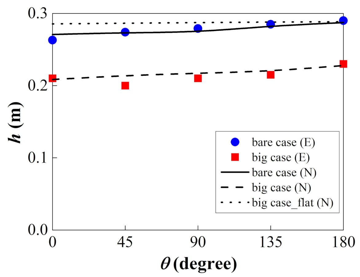
The transverse gradient at the channel curve caused by the centrifugal force is small and negligible due to the small quantity of flow and small radius of curvature. Therefore, the average depth of three sections (y/B = 0.25, y/B = 0.5 and y/B = 0.75) is calculated and shown in Figure 2 for four cases.
It can be seen from Figure 2 that the water depth changes less obviously along the curved reach for the bare case (smooth bed). As bed particles become larger, the sediment layer over the curved channel is thicker. At the conditions of the constant downstream water level at the tailgate, the thicker sediment layers lead to shallow water depth over the curved reach, i.e., in general. Therefore, the bed with the largest particle sizes leads to fastest mean flow velocity when the water depth at the tailgate is constant. In addition, the smaller discharge as shown in Figure 2a leads to less water depth differences for rough bed cases. As discharge becomes larger, water depth differences for rough bed cases are more apparent as provided in Figure 2c.
3.2. Longitudinal Velocity Distribution
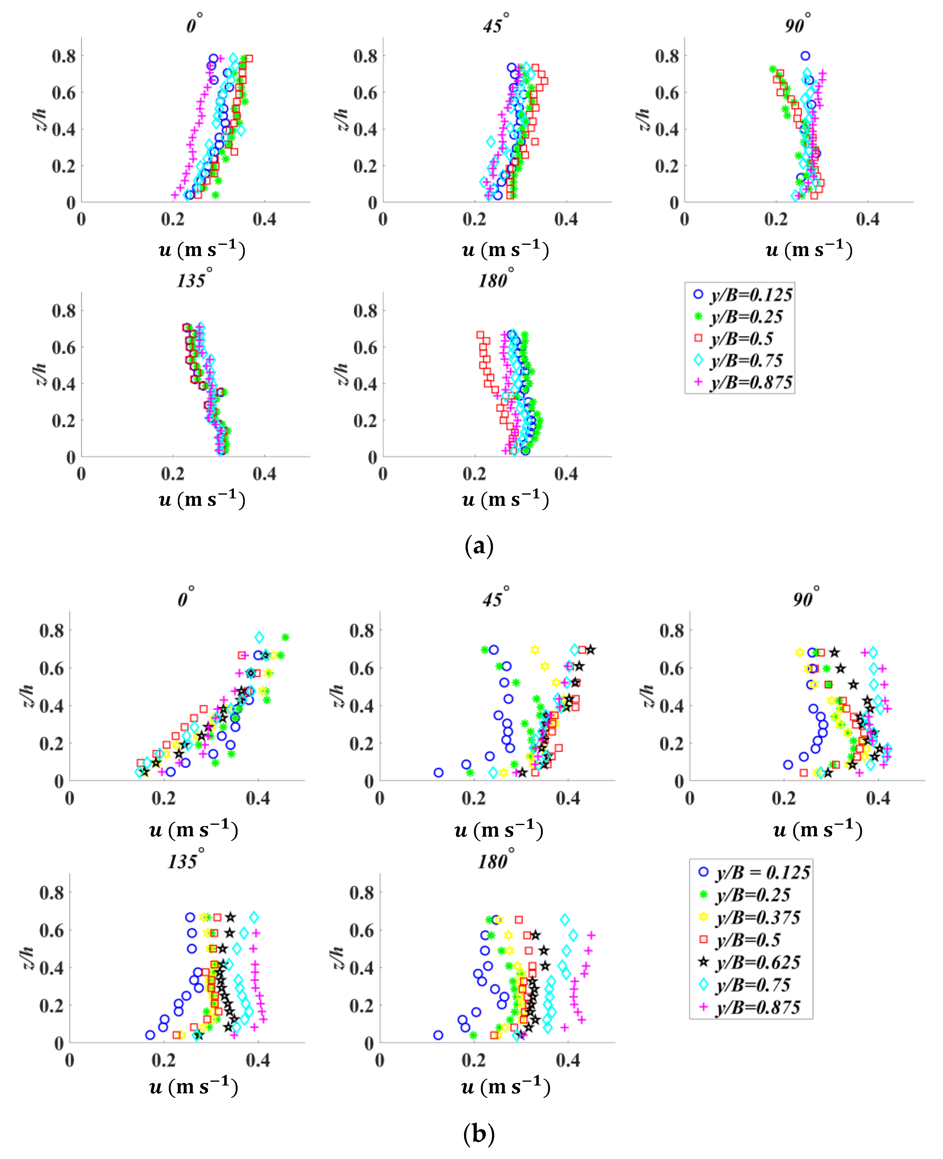
Figure 3 shows the longitudinal velocities along the depth of each section for smooth beds (bare case) and rough beds (small case, middle case and big case) for Q = 0.030 m3 s−1. For smooth bed (bare case, Figure 3a), the longitudinal velocity along the water depth at 0° and 45° sections follows logarithmic distribution, similar to the case in straight open channels. At the cross sections of 90° and 135°, the flow is affected by the channel bend. The longitudinal velocity gradually increases in the bottom region () and reduces in the top region (), thus breaking the logarithmic distribution law. Consequently, the longitudinal velocity as shown in Figure 3a exhibits an approximate “constant” distribution along the water depth as Blanckaert [37] and Barbhuiya and Talukdar [38] found.
For rough bed cases (Figure 3b–d), the longitudinal velocity profile is significantly different as the bare case. For the bare case, longitudinal velocity ranges from 0.2 m s−1 to 0.35 m s−1, while the values vary from 0.18 m s−1 to 0.45 m s−1 for the rough bed cases. Since the water depth at the tailgate is constant for all cases, the water depth with larger bed sediment particles becomes shallower, leading to greater longitudinal velocity. At 0° sections, the longitudinal velocity along the water depth also follows distinct logarithmic distribution, but the longitudinal velocity near the bed greatly decreases due to the bottom friction from rough bed, causing the steeper slope of the longitudinal velocity profile and larger induced bottom shear stress as other studies [15,23,39,40] mentioned. For the middle and big cases, the slope of the longitudinal velocity profile has little difference, which possibly means that the longitudinal velocity profile changes a little when the grain size reaches a certain level. At the 45° section, the longitudinal velocity profile near convex bank is affected by the channel bend firstly, implying that the longitudinal velocity gradually increases in the bottom and reduces near the water surface. However, the velocity profile near concave bank keeps following the logarithmic distribution. At the cross sections of 90° and 135°, the flow in the whole section is affected by the channel bend. Under the both effects of channel bend and rough bed, the longitudinal velocity distribution exhibits a trend of increasing near the bed and then decreasing near the surface along the water depth. It also can be found that the maximum longitudinal velocity at the central line occurs between 0.2 to 0.4 dimensionless depth from the bed. The grain size of bed particle only changes the magnitude of velocity, making the phenomena more remarkable. The trends of longitudinal velocity profiles for different rough bed cases are similar.
The velocity gradient between convex bank and concave bank for the bare case is unobvious. On the other hand, for the rough bed cases the transverse velocity gradient cannot be neglected, especially for the big case. The longitudinal velocity of concave bank is greater than that of convex bank for all rough bed cases, which indicates that the rough bed can enlarge the centrifugal effect of channel bend. Longitudinal velocity profiles for different flow discharge are similar and not discussed in detail here.
3.3. Turbulent Kinetic Energy and Power Spectral Density Analysis
In the study, TKE (k), represented as the turbulence characteristics, is defined as
where , and are the fluctuation velocities of u, v and w, respectively.
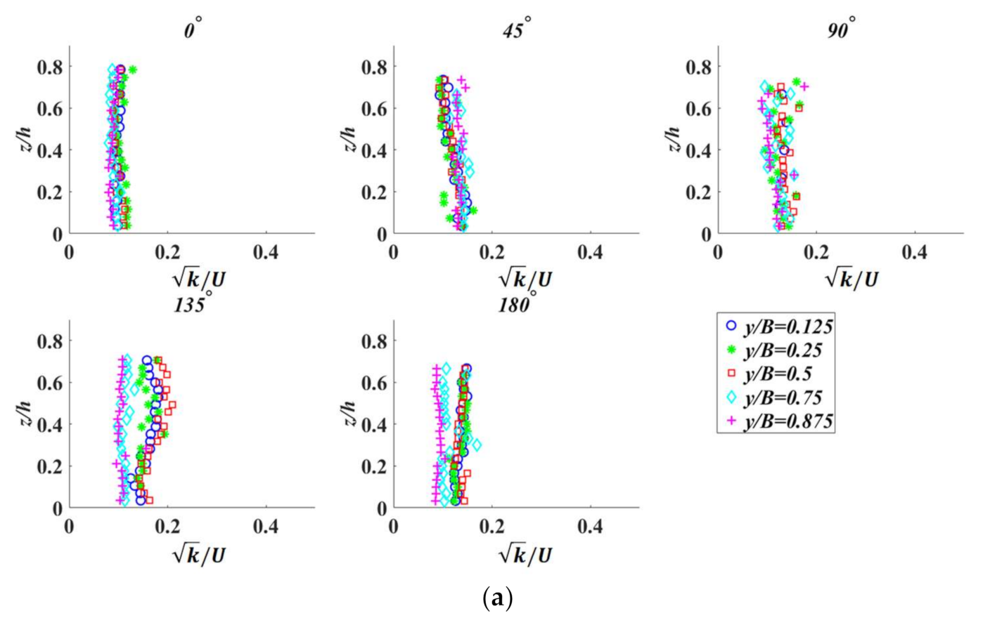
Taking Q = 0.030 m3 s−1 as an example, the TKE profiles, normalized by the overall mean velocity , under different tough bed conditions are shown in Figure 4. For the bare case (Figure 4a), the normalized k values show a constant distribution along the water depth for each cross section, but the normalized k values gradually increase from inlet (0° section) to the apex of bend (90° section) and decrease from the apex to outlet (180° section). The intense turbulence mainly concentrates in the cross section of 90°–135°. The reason is that the friction of the wall and the momentum exchange between the water flow and the wall leads to the increase of k values [4].
For the rough bed cases (Figure 4b–d), the normalized k values are smaller near the free surface, similar to the bare case. However, the normalized k values are larger near the bed region at the 0° section, implying that rough bed will enhance fluid mixing and strengthen turbulence as the results found in straight open channels [15,41]. The effect of bed roughness is not only confined for near bed regions but can be gradually extended to the whole water depth. As the particle size increases, the normalized k values near the bed increase a little because of the greater friction from the rough bed. Yet, the normalized k values near the surface remain basically unchanged. The slope of the variation of the normalized k values, i.e., , decreases, which means that at the same difference becomes larger. As a result, the rate in loss of k for larger particles becomes faster. After the 45° section, the normalized k values are also affected by the channel bend. Similar to the bare case, the normalized k values of the rough bed on the convex bank are larger than those for concave bank. Additionally, the vertical gradient of the variation of normalized k value increases, indicating that the rate in loss of k becomes slow. The k distributions for three rough bed cases are similar in curved channels. Therefore, the bed roughness and curved channel both improve turbulence along the water depth, especially near the bed regions. The effect of roughness is essential for the transport of the turbulent kinetic energy along the vertical direction.
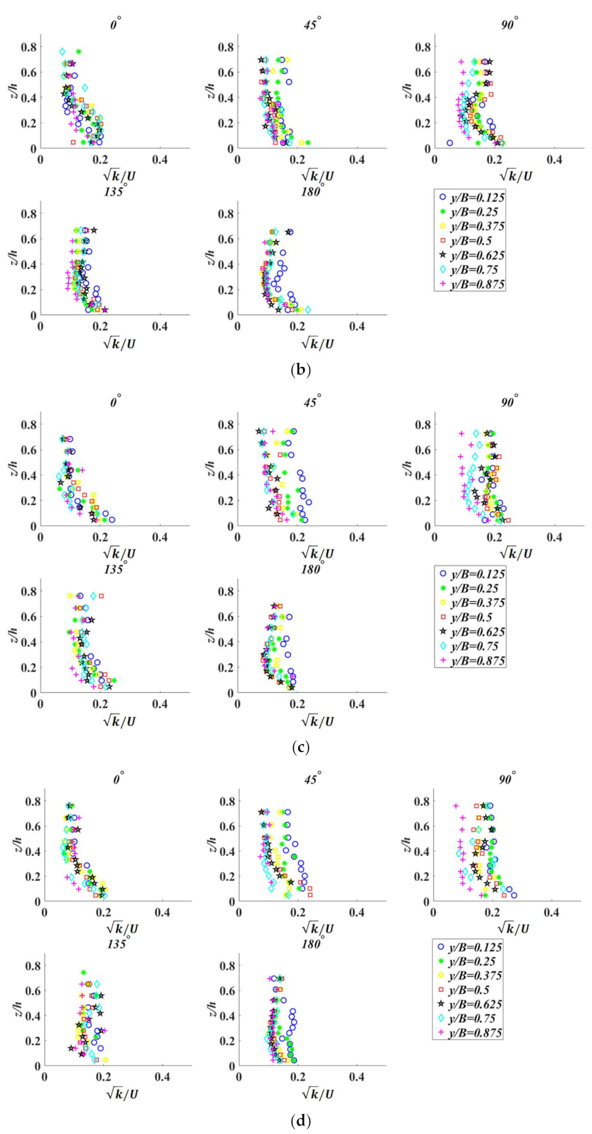
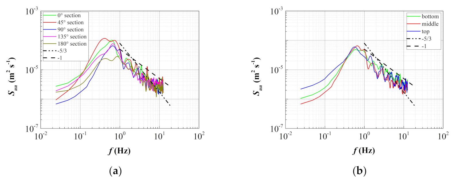
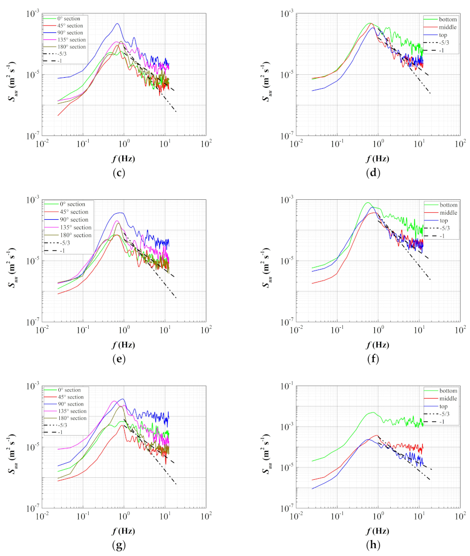
Figure 5 presents the variations in the power spectral density (PSD) of longitudinal velocity fluctuation with frequency f for different experimental conditions measured at the mid-width of the flume (20 cm from inner bank). Since the flow discharge has little effect on PSD, the discharge Q equal to 0.030 m3 s−1 is used as an example to reveal the variations of PSD. The spectral analysis used here is based on the Welch method with Hamming type windowing [42]. In Figure 5a,c,e,g, the feature point was measured at mid-depth (12 cm from the bed). In order to explore the effect of distance from the channel bed on PSD, three characteristic positions, i.e., 2 cm (bottom), 12 cm (middle) and 16 cm (top) from bed along the vertical direction, are provided at the 90° section in Figure 5b,d,f,h. Due to the limitation of ADV frequency, the energy input, inertial subrange and part of dissipation range can be observed. However, the higher frequency (part of dissipation range) is unable to present. Therefore, some of the small-scale turbulent structure can still be investigated.
For the bare case (Figure 5a), the PSD value for the high-frequency part at the 45° section is the greatest, while the PSD value at the 180° section is the smallest, indicating that the turbulence becomes strong, and the high-frequency (small-scale) vortex increases due to the influence of channel bend. For Figure 5b, there are similar trends for different positions for the bare case, which means the structures of turbulent vortex along vertical directions are approximately identical over smooth bed.
For the rough bed cases (Figure 5c,e,g), the PSD value for the high-frequency part at the 90° section is obviously larger than other sections. For Figure 5d,f,h, the PSD values at near-bed positions are larger than those at middle and top positions, and the trend is more prominent with the increasing bed particle size, implying that the turbulent mixing near the bed regions are more intense. The PSD of the longitudinal velocity fluctuations satisfy the classic Kolmogorov −5/3 law in the inertial subrange. Comparing to the bare case, the existence of bed roughness shortens the inertial subrange, causing the energy access to the viscous dissipation in advance. The peak frequency for each rough bed case is similar and about 0.8 Hz, irrespective of bed particle sizes.
3.4. Turbulent Bursting
It is found that fluid motion near a bed is not completely chaotic in nature, but it is a clear “sequence of ordered motion” [43]. Such coherent motions are called the bursting process [43]. To quantify the intermittent instantaneous Reynolds stresses as well as identify turbulence structures within a turbulent bursting sequence, one of the widely used conditional sampling techniques is the quadrant analysis of the Reynolds shear stress [44,45,46]. Here, quadrant analysis was conducted to study the effect of rough bed on turbulent bursting. In the quadrant analysis, the Reynolds stress has four types of contributions according to the signs of the instantaneous velocity fluctuations [42]. Accordingly, turbulent events are defined by the four quadrants as outward interactions (), ejections (), inward interactions (), and sweeps (). Results in quadrants II and IV mean the positive downward momentum flux and are involved in turbulence near-bed bursting [43].
In order to describe the turbulent event accurately, the hole (instead of zero) concept is used to eliminate smaller Reynolds stresses. The hole is formed by four hyperbolas , where is a threshold value. By using the threshold, small values can be ignored in the i-th quadrant [47]. The contribution of each quadrant can be represented as (k = I, II, III, IV, indicate the four quadrants), where
In the study, the threshold was set to 1.0 [48]. Then, the revised occurrence frequency, fk, for the four turbulent events is given as:
where T is the length of measurement time.
Figure 6 shows characteristic distributions of the occurrence frequency fk in different cases for Q = 0.030 m3 s−1 as an example. The feature point is measured at the distance of 0.01 m from the bed in the vertical direction and 0.20 m from the inner bank (center of the flume) in the transverse direction in each section to investigate the turbulent event near bed. For the bare case (Figure 6a), it can be observed that sweep and ejection events (event II and IV) occur with comparable frequency and are much higher than outward and inward interactions at the 0° section, indicating that upwards motion of low-speed fluid and downwards motion of high-speed fluid are dominant. After the 45° section, the frequency of occurrence of events of I and III quadrants become higher. At the 180° section, the frequency of occurrence for four events is similar. This reveals that high-speed fluid reflects by the bottom and low-speed fluid is pushed back as the influence of channel bend, showing a strong interaction of the turbulent structures with the main flow. For rough bed cases, it is noted that higher magnitude of sweep and ejections (event II and IV) contributions as shown in Figure 6b (small case) similar to the bare case at the 0° section. When flow enters the curved channel, the frequency of occurrence for event II and IV increases, indicating that sweep and ejection are the most dominant processes, which can potentially influence the sediment transport in the stream, causing the exchange of energy and momentum in the flow and the bed formation. The middle case (Figure 6c) performs the similar trend as the small case. However, for the big case (Figure 6d) the frequency of occurrence for event II and IV decreases first (0° section to 90° section) and then increases (90° section to 180° section). Therefore, the contributions of sweeps and ejections are more important than those of the outward and inward interactions over a rough bed, which are the same results obtained by other researches in straight channels [43,49]. Bed roughness is the leading factor to the turbulent bursting in curved channels when the grain size of bed particles is moderate (the small case and middle case), but for the big case the turbulent bursting is weaken before the apex of the bend. The possible explanation is the larger grain size of bed particles possible disturbs the bottom boundary layer, changing turbulent structure near the bed.
3.5. Comparisons with Previous Experimental Results
All of the experiment cases in this paper were done in a 180 degree U-shaped curved and rough bed flume under the condition of constant downstream water level, close to the practical situations on the purpose of navigation. Thus, the experimental results in comparison with previous studies may have some differences. Firstly, since the downstream water level is fixed, as the bed particles become larger, the water depth along the curved channel decreases, leading to greater velocity compared with that over smooth curved channels. Without the constant downstream water depth, the water depth along the curved channel may keep similar [18]. Secondly, the longitudinal velocity distribution is relatively different. Pradhan et al. [20] found that the velocity remains higher towards the inner wall for rough bed. In our experimental results, longitudinal velocity near the concave bank is greater than that near the convex bank for all rough bed cases, which indicates that the rough bed can enlarge the centrifugal effect of channel bend. The reason may be the different shape of cross-section of channel (trapezoidal channel for Pradhan et al. [20]). Thirdly, sweeps and ejections are more important than those of the outward and inward interactions over a rough bed when the grain size of bed particles is intermediate [43,49]. For the big case, the proportion of the outward and inward interactions is higher than that of the sweeps and ejections in 90° section, which was not shown in the results of Najafabadi et al. [43] because of the limits of the grain size in the study.
3.6. Numerical Results
Numerical tests aim to understand the effect of thick sediment layers on secondary flow over a curved channel. The roughness height ks of the FLOW-3D simulation was adjusted until the numerical results close to experimental data. The roughness height ks = 0.005 m for the bare case and the roughness height ks = 0.05 m for the big case can match well with the experimental water depths and longitudinal velocity as shown in Figure 7 and Figure 8. The differences between the simulation and measurements can be possibly attributed to three aspects: (1) the isotropic assumptions in the RNG turbulence model are not suitable for curved channel flows, (2) the uneven bottom surface from sediment particles and flows through pores between sediment particles are unable to reflect in the numerical tests, where the solid step is used to represent the sediment layers, and (3) the slope of the entire channel may not be constant. For big case_flat, the water depth increases a little due to the bottom friction from rough bed, and the water depth of each section is approximately the same, i.e., uniform flow conditions, meaning that the friction exerted by the rough bed mainly balances gravity due to sloping bed.
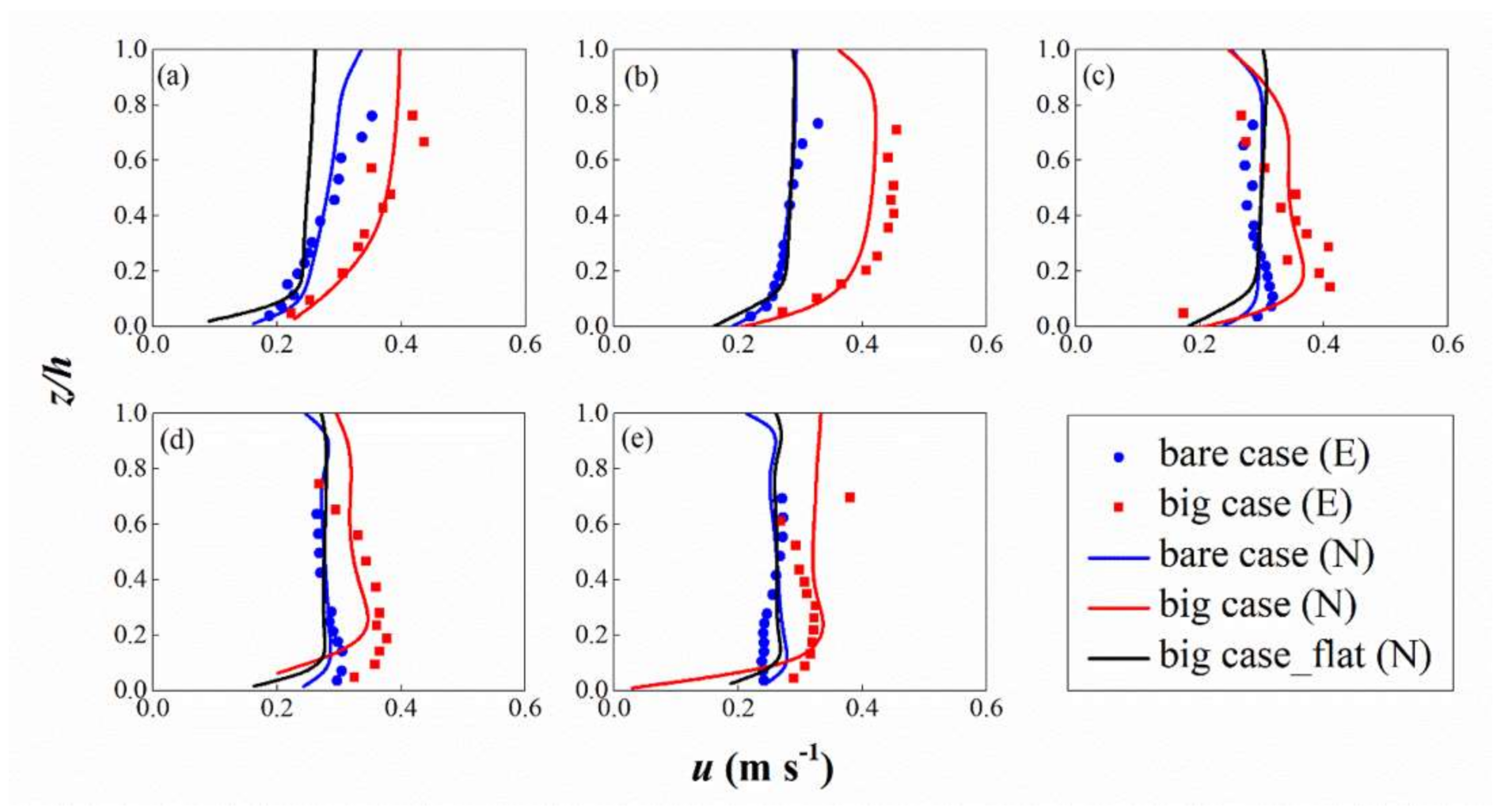
Figure 8 performs the longitudinal velocity profiles at the mid-width of the flume (20 cm from inner bank) under different cases. The simulated velocity distribution at the 90° and 135° section does not fit very well with the experimental results, especially for the big case. For big case_flat, the longitudinal velocity near bed decreases due to the bed friction when compared with the bare case. On the other hand, the longitudinal velocity for the big case_flat is smaller than that for the big case owing to larger water depths.
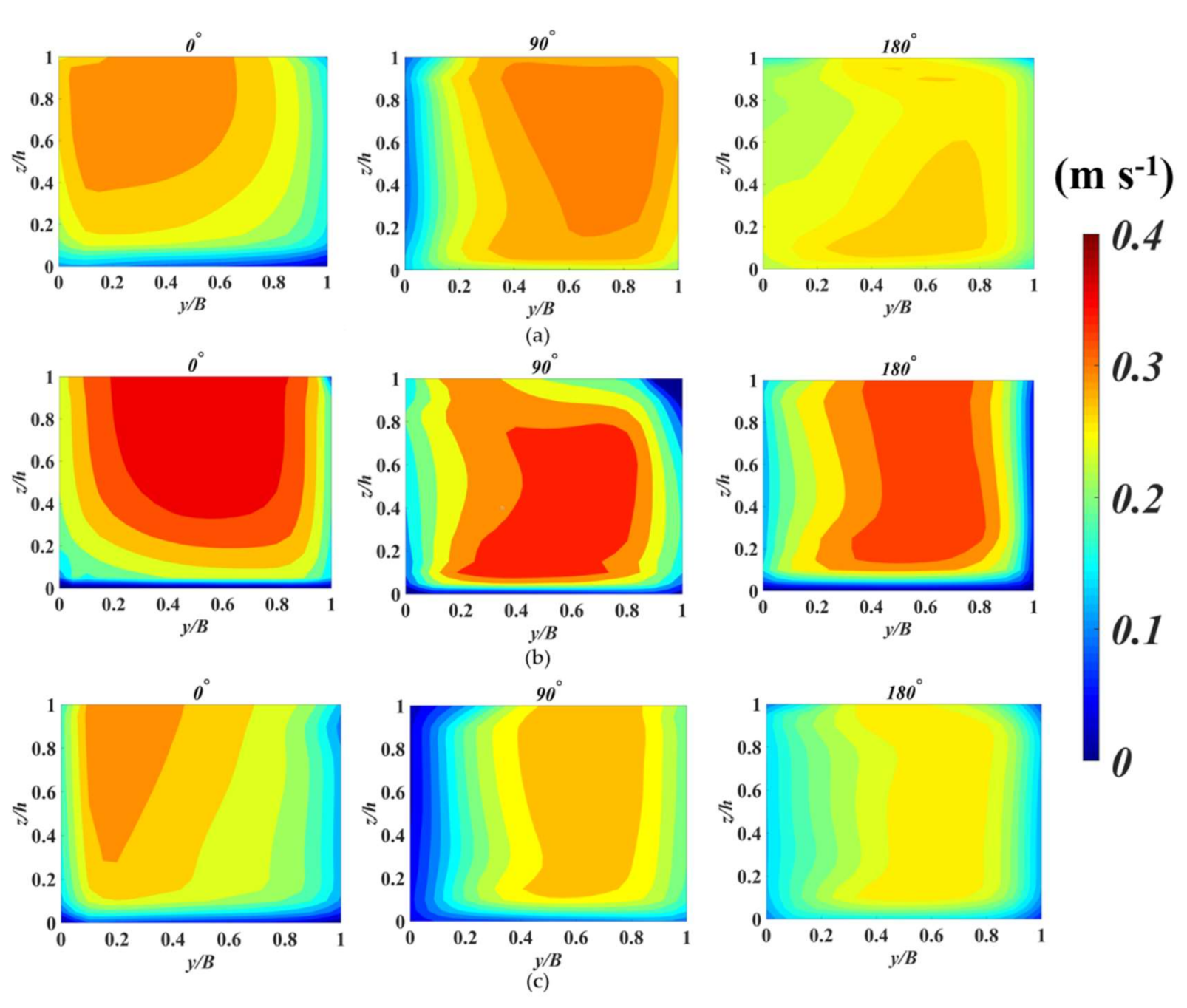
The distributions of longitudinal velocity in three typical cross-sections (0°, 90° and 180°) are shown in Figure 9. For the bare case (Figure 9a), the core region of maximum longitudinal velocity has obviously shifted toward the concave bank at the 90° and 180° section in comparison with that at the 0° section. This is because of the advective transport of streamwise momentum by the cross-stream circulation in open-channel bends. At the bend entrance, the shorter distance in the inner bend than that in the outer bend would lead to longitudinal velocity u decreasing from the convex toward the concave bank. The flow acceleration/deceleration is induced by streamwise pressure gradients related to the sudden transverse tilting of the water surface in the bend. In addition, the sudden disappearance of the transverse tilting of the water surface leads to pronounced flow accelerations/deceleration in the concave/convex bend at the bend exit [3,50]. For the big case (Figure 9b), the core region of maximum longitudinal velocity stays around the center region of the cross-section at the 0° and 90° sections. At the 180° section, the core region shifts to the concave bank. For the big case_flat (Figure 9c), numerical results are similar to that for the bare case at the 0° and 90° sections. However, at the 180° section, the maximum longitudinal velocity for the big case_flat concentrates on the right middle region rather than the lower right region for the bare case. Based upon the results, it can be concluded that thick sediment layers delay the shifting of the core of maximum longitudinal velocity towards the concave bank. The bed roughness only reduces the longitudinal velocity magnitude.
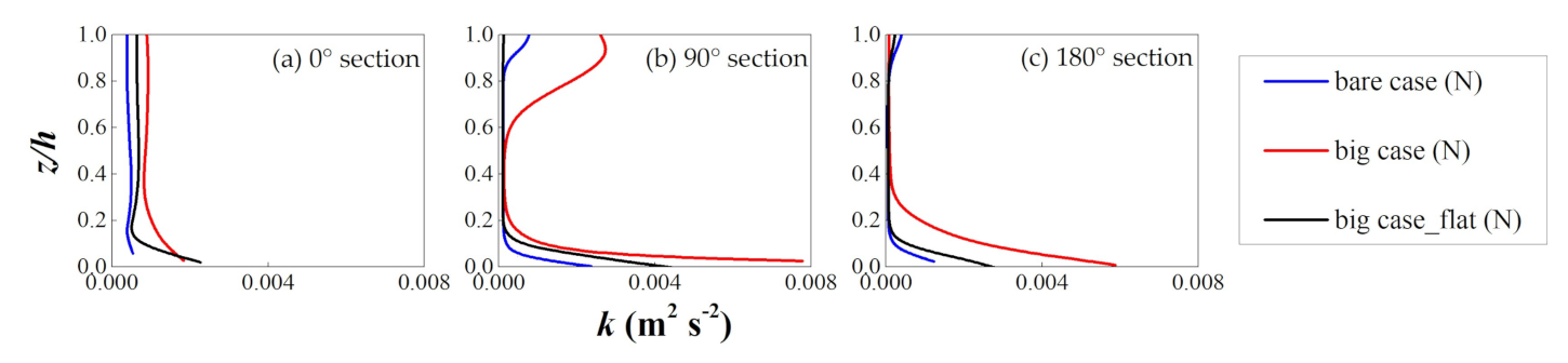
The distributions of k at the mid-width of the flume (20 cm from inner bank) at three typical cross-sections (0°, 90° and 180°) are shown in Figure 10. For the 0° section (Figure 10a), the k values of three cases are smaller near the free surface but become larger near the rough bed regions, implying that rough bed will enhance fluid mixing and strengthen turbulence. Additionally, the k values of the big case_flat are slightly larger than those of the big case. For the 90° and 180° sections (Figure 10b,c), the k values firstly increase (from 0° section to 90° section) and then decrease (from 90° section to 180° section), indicating that the channel bend can also improve turbulence along the water depth, especially near the bed regions. However, the k values of the big case (red line) increase more than the other two cases along the curved channel. The result suggests that the bed roughness and curved channel both improve turbulence along the water depth, especially near the bed regions, which is the same as the experimental results. Additionally, the thick sediment layer can promote TKE more than the curved channel does.
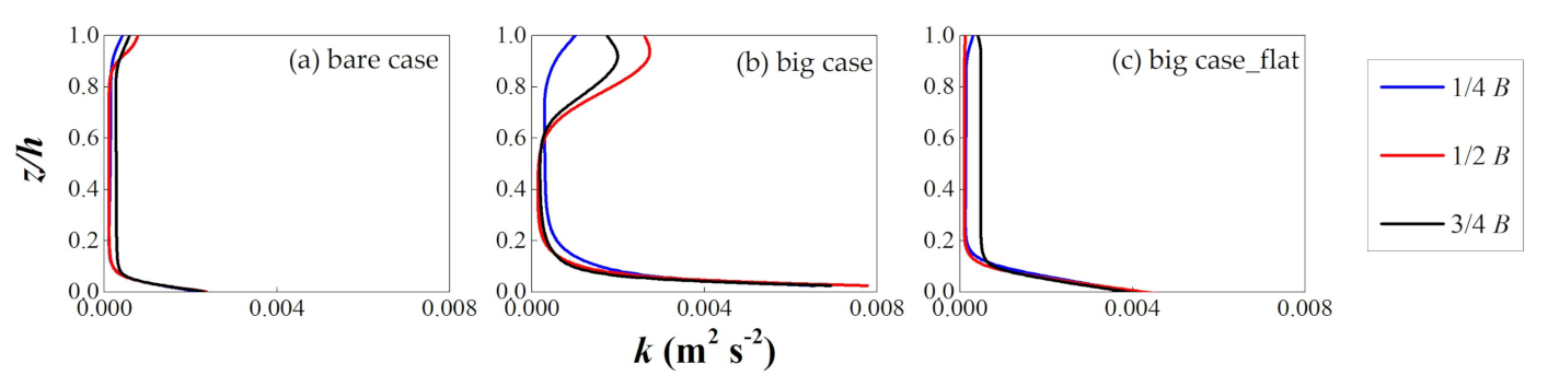
In order to explore the effect of distance from the convex bank on the distributions of k, three characteristic positions, i.e., ¼cm (=1/4 B), ½cm (=1/2 B) and ¾cm (=3/4 B) from the convex bank along the transverse direction, are provided at the 90° section for three cases as shown in Figure 11. For the bare case (Figure 11a), the k values of three lines basically collapse together, meaning that the transverse positive has little effect to the k values for the smooth bed. For the big case (Figure 11b), the k values near convex bank is slightly larger when z/h = 0.1–0.6. The thick sediment layer with bed roughness strengthens the turbulence more near convex bank, which is the same as the experimental result. However, for the big case_flat (Figure 11c), the k values near concave bank at z/h > 0.1 is larger. The thick sediment layer increases the TKE (k) values, especially near convex bank.
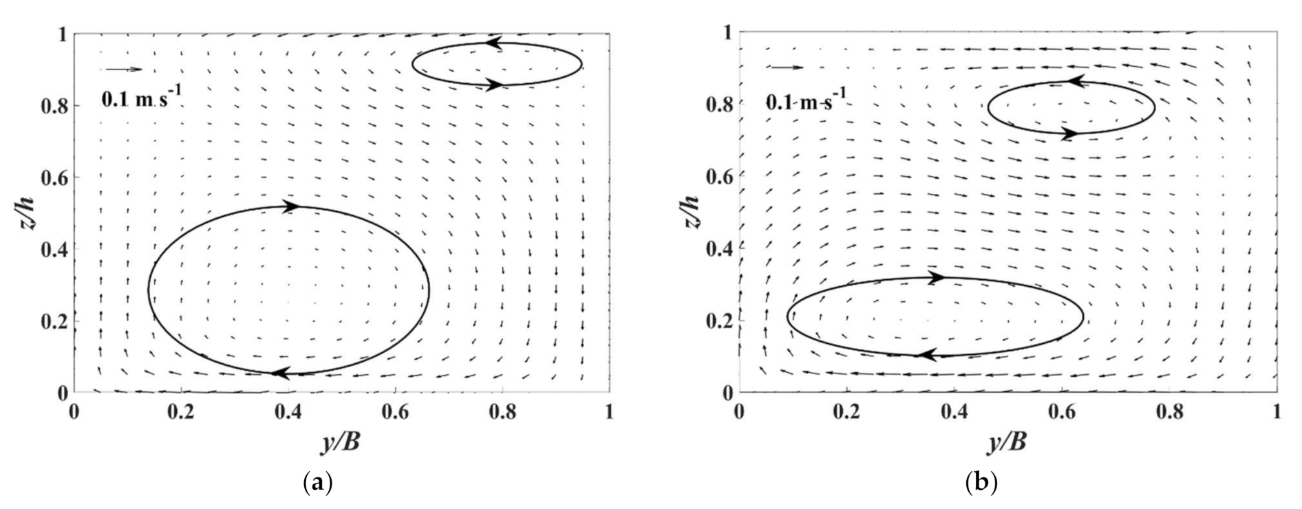
The secondary flow that can interact dynamically with the primary flow is important for meandering rivers and useful for studies of diffusion and navigation in natural waterways, because it is partly responsible for the large-scale bed topography of natural alluvial channel bends [51]. The vector of the cross-stream motion (v, w) at the 90° section is shown in Figure 12. For the bare case (Figure 12a), there is a classical helical motion obviously, called the center-region cell. In addition, a weaker counterrotating cell of cross-stream circulation, called the outer-bank cell, exists in the corner formed by the water surface and the outer bank as Blanckaert and Graf [2] revealed. The center-region cell plays an important role in the advective momentum transport, and the outer-bank cell is believed to be crucial to bank erosion processes [52]. For the big case (Figure 12b), the center-region cell and outer-bank cell still exist. The center-region cell is confined to the near-bed area, and the outer-bank cell is stronger than that for the bare case, possibly accelerating the bank erosion. This is because the rough bed disturbs the flow, mainly reducing the longitudinal flow velocity near bed, and also affecting the distribution of the transverse velocity along the water depth. For the big case_flat (Figure 12c), the center-region cell is confined to a smaller area compared to the bare and big cases, which means that the thick sediment layer can influence more riverbed regions. Furthermore, the outer-bank cell is weaker than that for the big case.
The transverse velocity distribution can be used to display the intensity of secondary flow. Figure 13 shows the secondary flow distributions of different cases at the mid-width of the flume (20 cm from inner bank) at the 90° section, where X-axis is , Y-axis is , r is curvature radius of bend, and is average longitudinal velocity. When the calculated values () distribute on the same side of = 0, i.e., all values are larger or smaller than zero, it means that the direction of transverse velocity is the same at this position. In other words, there is no secondary flow. Once the calculated values () fall on the two sides of = 0, there is secondary flow existing. Additionally, the secondary flow is stronger as the slope of transverse velocity distribution increases.
From Figure 13, it can be seen that numerical simulations (solid line) are close to experimental measurements (individual symbols). The slope of transverse velocity distribution for the big case is steeper than that for the bare case, which means that the rough bed would strengthen the secondary flow and possibly causes more riverbed erosion. Besides, the position of calculated values ( = 0) for the big case is lower than that of the bare case, representing the secondary flow is confined to the near-bed area as the results discussed above. For the big case and big case_flat, the slope of transverse velocity distribution is comparable, i.e., similar secondary flow intensity.
4. Conclusions
Experiments and numerical simulation of curved open channel flows over rough beds under the condition of constant downstream water depth were carried out. Based on the ADV data, hydrodynamic characteristics of flow over rough bed such as longitudinal velocity distribution, turbulent characteristics, secondary flow, turbulent bursting and so on was analyzed. Additionally, the numerical results were used to show different flow patterns for the rough bed with and without thick sediment layers. The following conclusions are drawn:
- In the study, the experiments cases were carried in a 180 degree U-shaped curved and rough bed flume under the condition of constant downstream water level. Different as previous studies, as the bed particles become larger, the water depth along the curved channel decreases, leading to greater velocity compared with that over smooth curved channels. The longitudinal velocity near bed significantly decreases due to the existence of rough bed, resulting in the larger gradient of longitudinal velocity profile for rough bed than that in the bare case. As the both effect of channel bend and rough bed, the longitudinal velocity profiles exhibit a trend of increasing in the bottom and decreasing near the water surface. The grain size of bed particles only changes the magnitude of velocity, making the phenomena more remarkable. Rough bed also enlarges the centrifugal effect of channel bend, and as a result the longitudinal velocity of concave bank is higher than that of convex bank.
- Rough bed will enhance the mixing between the water bodies and rough bed, strengthening turbulence and increasing turbulent kinetic energy. From the power spectral density analysis, the structure of turbulent vortex along the vertical direction is resembled. However, the turbulent energy of near-bed position is bigger than that of top position. The power spectra of the longitudinal velocity components follow the classic Kolmogorov -5/3 law in the inertial subrange, and the existence of rough bed shortens the inertial subrange and reaches to the viscous dissipation in advance.
- The contributions of sweeps and ejections are more important than those of the outward and inward interactions over a rough bed. In addition, bed roughness is the dominant factor to the turbulent bursting in curved channels when the grain size of bed particles is intermediate (the small case and middle case), but the influence of rough bed for the big case to the turbulent bursting weakens due to the disturbances of bottom boundary layer.
- Numerical simulations were used to discuss flow patterns over two different rough bed settings (the big and big_flat cases). Since the bed surface roughness are the same for the two cases, their skin drag to flow is identical. However, the form drag is greater for bed covered with a thick sediment layer (the big case) rather than the flat bed (the big_flat case). Simulation results show that for both rough bed cases the secondary flow is confined to the near-bed area and the intensity of secondary flow is improved, possibly causing more serious bed erosion along a curved channel. As a result, the advective momentum transport increases over rough and curved channels. Furthermore, the thick sediment layer (the big case), i.e., larger form drag, can delay the shifting of the core region of maximum longitudinal velocity towards the concave bank.
- The effect of rough bed to turbulent kinetic energy is also provided using numerical methods. The numerical results show that the thick sediment layer can lead to larger k values than the curved channel and increase the TKE (k) values, especially near convex bank.
The findings of the research could improve the understanding of the interactive effects between the rough bed and the strongly curved channel flow. Based on the reported results, future researches can focus on studying the effect of flume curvature on the hydrodynamic characteristics of curved channel flow with gravel beds.
Author Contributions
Conceptualization, Y.-J.C., Y.-T.L. and X.J.; Methodology, Y.-J.C. and Y.-T.L.; Laboratory measurement, Y.Y.; Data analysis, Y.-T.L. and Y.Y.; Writing—Original Draft Preparation, Y.-T.L. and Y.Y.; Writing—Review and Editing, Y.-J.C.; Software, X.J.; Funding Acquisition, Y.-J.C. and X.J. All authors have read and agreed to the published version of the manuscript.
Funding
This research was funded by National Key Research and Development Project of China [grant number 2017YFC0405205]; Ministry of Science and Technology of Taiwan [grant number MOST 109-2625-M-002-016]; Zhejiang Provincial Natural Science Foundation of China [grant number LY20A020009); State Key Laboratory of Hydraulic Engineering Simulation and Safety, Tianjin University [grant number HESS-2014]; Fundamental Research Funds for the Central Universities [grant number 2020QNA4038].
Institutional Review Board Statement
Not applicable.
Informed Consent Statement
Not applicable.
Data Availability Statement
All data generated or analyzed during this study are included in this article.
Conflicts of Interest
The authors declare no conflict of interest.
References
- Wei, M.; Blanckaert, K.; Heyman, J.; Li, D.; Schleiss, A.J. A parametrical study on secondary flow in sharp open-channel bends: Experiments and theoretical modelling. J. Hydro-Environ. Res. 2016, 13, 1–13. [Google Scholar] [CrossRef]
- Blanckaert, K.; Graf, W.H. Momentum transport in sharp open-channel bends. J. Hydraul. Eng. 2004, 130, 186–198. [Google Scholar] [CrossRef]
- Zeng, J.; Constantinescu, G.; Blanckaert, K.; Weber, L. Flow and bathymetry in sharp open-channel bends: Experiments and predictions. Water Resour. Res. 2008, 44, W09401. [Google Scholar] [CrossRef]
- Blanckaert, K. Topographic steering, flow recirculation, velocity redistribution, and bed topography in sharp meander bends. Water Resour. Res. 2010, 46, W09506. [Google Scholar] [CrossRef]
- Blanckaert, K.; De Vriend, H.J. Meander dynamics: A nonlinear model without curvature restrictions for flow in open-channel bends. J. Geophys. Res.-Earth Surf. 2010, 115, F04011. [Google Scholar] [CrossRef] [Green Version]
- Vaghefi, M.; Akbari, M.; Fiouz, A.R. An experimental study of mean and turbulent flow in a 180 degree sharp open channel bend: Secondary flow and bed shear stress. KSCE J. Civ. Eng. 2016, 20, 1582–1593. [Google Scholar] [CrossRef]
- Bomminayuni, S.; Stoesser, T. Turbulence statistics in an open-channel flow over a rough bed. J. Hydraul. Eng. 2011, 137, 1347–1358. [Google Scholar] [CrossRef]
- Grass, A.J.; Stuart, R.J.; Mansour-Tehrani, M. Vortical structures and coherent motion in turbulent flow over smooth and rough boundaries. Philos. Trans. R. Soc. Lond. A 1991, 336, 35–65. [Google Scholar] [CrossRef]
- Ferro, V. Friction factor for gravel-bed channel with high boulder concentration. J. Hydraul. Eng. 1999, 125, 771–778. [Google Scholar] [CrossRef]
- Ferro, V. Flow resistance in gravel-bed channels with large-scale roughness. Earth Surf. Process. Landf. 2003, 28, 1325–1339. [Google Scholar] [CrossRef]
- Nikora, V.; Goring, D.; McEwan, I.; Griffiths, G. Spatially averaged open-channel flow over rough bed. J. Hydraul. Eng. 2001, 127, 123–133. [Google Scholar] [CrossRef]
- Nikora, V.; Koll, K.; McEwan, I.; McLean, S.; Dittrich, A. Velocity distribution in the roughness layer of rough-bed flows. J. Hydraul. Eng. 2004, 130, 1036–1042. [Google Scholar] [CrossRef]
- Mignot, E.; Barthélemy, E.; Hurther, D. Double-averaging analysis and local flow characterization of near-bed turbulence in gravel-bed channel flows. J. Fluid Mech. 2009, 618, 279–303. [Google Scholar] [CrossRef]
- Dey, S.; Das, R.; Gaudio, R.; Bose, S.K. Turbulence in mobile-bed streams. Acta Geophys. 2012, 60, 1547–1588. [Google Scholar] [CrossRef]
- Qi, M.; Li, J.; Chen, Q.; Zhang, Q. Roughness effects on near-wall turbulence modelling for open-channel flows. J. Hydraul. Res. 2018, 56, 648–661. [Google Scholar] [CrossRef]
- Jin, Y.; Steffler, P.M.; Hicks, F.E. Roughness effects on flow and shear stress near outside bank of curved channel. J. Hydraul. Eng. 1990, 116, 563–577. [Google Scholar] [CrossRef]
- Blanckaert, K.; Duarte, A.; Chen, Q.; Schleiss, A.J. Flow processes near smooth and rough (concave) outer banks in curved open channels. J. Geophys. Res.-Earth Surf. 2012, 117, F04020. [Google Scholar] [CrossRef] [Green Version]
- Hersberger, D.S.; Franca, M.J.; Schleiss, A.J. Wall-roughness effects on flow and scouring in curved channels with gravel beds. J. Hydraul. Eng. 2016, 142, 4015032. [Google Scholar] [CrossRef]
- Jamieson, E.C.; Post, G.; Rennie, C.D. Spatial variability of three-dimensional Reynolds stresses in a developing channel bend. Earth Surf. Process. Landf. 2010, 35, 1029–1043. [Google Scholar] [CrossRef]
- Pradhan, A.; Kumar Khatua, K.; Sankalp, S. Variation of velocity distribution in rough meandering channels. Adv. Civ. Eng. 2018, 2018, 1–12. [Google Scholar] [CrossRef]
- Kraus, N.C.; Lohrmann, A.; Cabrera, R. New acoustic meter for measuring 3D laboratory flows. J. Hydraul. Eng. 1994, 120, 406–412. [Google Scholar] [CrossRef]
- Goring, D.G.; Nikora, V.I. Despiking acoustic doppler velocimeter data. J. Hydraul. Eng. 2002, 128, 117–126. [Google Scholar] [CrossRef] [Green Version]
- Wang, X.; Yang, Q.; Lu, W.; Wang, X. Experimental study of near-wall turbulent characteristics in an open-channel with gravel bed using an acoustic doppler velocimeter. Exp. Fluids 2012, 52, 85–94. [Google Scholar] [CrossRef]
- Li, C.; Xue, W.; Huai, W. Effect of vegetation on flow structure and dispersion in strongly curved channels. J. Hydrodyn. 2015, 27, 286–291. [Google Scholar] [CrossRef]
- Nogueira, H.I.S.; Adduce, C.; Alves, E.; Franca, M.J. Analysis of lock-exchange gravity currents over smooth and rough beds. J. Hydraul. Res. 2013, 51, 417–431. [Google Scholar] [CrossRef]
- Yalin, M.S. River Mechanics; Elsevier Science & Technology: Kent, UK, 1992. [Google Scholar]
- Schlichting, H.; Gersten, K. Boundary-Layer Theory, 8th ed.; Springer: Berlin, Germany, 2000. [Google Scholar]
- Kironoto, B.A.; Graf, W.H. Turbulence characteristics in rough uniform open-channel flow. Proc. Inst. Civ. Eng. Water Marit. Energy 1994, 106, 333–344. [Google Scholar] [CrossRef]
- Glatzel, T.; Litterst, C.; Cupelli, C.; Lindemann, T.; Moosmann, C.; Niekrawietz, R.; Streule, W.; Zengerle, R.; Koltay, P. Computational fluid dynamics (CFD) software tools for microfluidic applications—A case study. Comput. Fluids 2008, 37, 218–235. [Google Scholar] [CrossRef]
- Al-Qadami, E.H.H.; Abdurrasheed, A.S.; Mustaffa, Z.; Yusof, K.W.; Malek, M.A.; Ghani, A.A. Numerical modelling of flow characteristics over sharp crested triangular hump. Results Eng. 2019, 4, 100052. [Google Scholar] [CrossRef]
- Ghaderi, A.; Dasineh, M.; Aristodemo, F.; Aricò, C. Numerical simulations of the flow field of a submerged hydraulic jump over triangular macroroughnesses. Water 2021, 13, 674. [Google Scholar] [CrossRef]
- Qi, H.; Zheng, J.; Zhang, C. Modeling excess shear stress around tandem piers of the longitudinal bridge by computational fluid dynamics. J. Appl. Water Eng. Res. 2021. [Google Scholar] [CrossRef]
- Huang, T.; Jan, C.; Hsu, Y. Numerical simulations of water surface profiles and vortex structure in a vortex settling basin by using flow-3d. J. Mar. Sci. Technol. 2017, 25, 531–542. [Google Scholar] [CrossRef]
- Abbaspour, A.; Kia, S.H. Numerical investigation of turbulent open channel flow with semi-cylindrical rough beds. KSCE J. Civ. Eng. 2014, 18, 2252–2260. [Google Scholar] [CrossRef]
- Bai, Y.; Song, X.; Gao, S. Efficient investigation on fully developed flow in a mildly curved 180° open-channel. J. Hydroinform. 2014, 16, 1250–1264. [Google Scholar] [CrossRef]
- Gholami, A.; Akhtari, A.A.; Minatour, Y.; Bonakdari, H.; Javadi, A.A. Experimental and numerical study on velocity fields and water surface profile in a strongly-curved 90 degrees open channel bend. Eng. Appl. Comp. Fluid Mech. 2014, 8, 447–461. [Google Scholar] [CrossRef] [Green Version]
- Blanckaert, K. Flow and Turbulence in Sharp Open Channel Bends. Ph.D. Thesis, Ecole Polytechnique Fédérale de Lausanne, Lausanne, Switzerland, 2003. [Google Scholar]
- Barbhuiya, A.K.; Talukdar, S. Scour and three dimensional turbulent flow fields measured by ADV at a 90 ° horizontal forced bend in a rectangular channel. Flow Meas. Instrum. 2010, 21, 312–321. [Google Scholar] [CrossRef]
- Singh, K.M.; Sandham, N.D.; Williams, J.J.R. Numerical simulation of flow over a rough bed. J. Hydraul. Eng. 2007, 133, 386–398. [Google Scholar] [CrossRef] [Green Version]
- Reidenbach, M.A.; Limm, M.; Hondzo, M.; Stacey, M.T. Effects of bed roughness on boundary layer mixing and mass flux across the sediment-water interface. Water Resour. Res. 2010, 46, 58–72. [Google Scholar] [CrossRef]
- Jiménez, J. Turbulent flows over rough walls. Annu. Rev. Fluid Mech. 2004, 36, 173–196. [Google Scholar] [CrossRef]
- Huai, W.; Zhang, J.; Wang, W.; Katul, G.G. Turbulence structure in open channel flow with partially covered artificial emergent vegetation. J. Hydrol. 2019, 573, 180–193. [Google Scholar] [CrossRef]
- Najafabadi, E.F.; Afzalimehr, H.; Sui, J. Turbulence characteristics of favorable pressure gradient flows in gravel-bed channel with vegetated walls. J. Hydrol. Hydromech. 2015, 63, 154–163. [Google Scholar] [CrossRef] [Green Version]
- Mazumder, B.S.; Pal, D.K.; Ghoshal, K.; Ojha, S.P. Turbulence statistics of flow over isolated scalene and isosceles triangular-shaped bedforms. J. Hydraul. Res. 2009, 47, 626–637. [Google Scholar] [CrossRef]
- Kassem, H.; Thompson, C.E.L.; Amos, C.L.; Townend, I.H. Wave-induced coherent turbulence structures and sediment resuspension in the nearshore of a prototype-scale sandy barrier beach. Cont. Shelf Res. 2015, 109, 78–94. [Google Scholar] [CrossRef] [Green Version]
- Li, Y.; Wei, J.; Gao, X.; Chen, D.; Weng, S.; Du, W.; Wang, W.; Wang, J.; Tang, C.; Zhang, S. Turbulent bursting and sediment resuspension in hyper-eutrophic Lake Taihu, China. J. Hydrol. 2018, 565, 581–588. [Google Scholar] [CrossRef]
- Lu, S.S.; Willmarth, W.W. Measurements of the structure of the Reynolds stress in a turbulent boundary layer. J. Fluid Mech. 1973, 60, 481–511. [Google Scholar] [CrossRef]
- Duan, J.; He, L.; Wang, G.; Fu, X. Turbulent burst around experimental spur dike. Int. J. Sediment Res. 2011, 26, 471–486. [Google Scholar] [CrossRef]
- Keshavarzy, A.; Ball, J.E. An analysis of the characteristics of rough bed turbulent shear stresses in an open channel. Stoch. Hydrol. Hydraul. 1997, 11, 193–210. [Google Scholar] [CrossRef]
- Henderson, F.M. Open Channel Flows; Macmillan: New York, NY, USA, 1966. [Google Scholar]
- Falcon, M. Secondary flow in curved open channels. Annu. Rev. Fluid Mech. 1984, 16, 179–193. [Google Scholar] [CrossRef]
- Blanckaert, K.; De Vriend, H.J. Secondary flow in sharp open-channel bends. J. Fluid Mech. 2004, 498, 353–380. [Google Scholar] [CrossRef] [Green Version]
Figure 1.
Scheme of experiment setup: (a) The shadow shows rough bed regions and the inset figure represents rough bed configurations; (b) ADV measurement setup.
Figure 1.
Scheme of experiment setup: (a) The shadow shows rough bed regions and the inset figure represents rough bed configurations; (b) ADV measurement setup.

Figure 2.
Water depth variations along the curved reach for four cases: (a) Q = 0.015 m3 s−1, (b) Q = 0.025 m3 s−1, and (c) Q = 0.030 m3 s−1 (● Bare case; ■ Small case; ▲ Middle case; ♦ Big case).
Figure 2.
Water depth variations along the curved reach for four cases: (a) Q = 0.015 m3 s−1, (b) Q = 0.025 m3 s−1, and (c) Q = 0.030 m3 s−1 (● Bare case; ■ Small case; ▲ Middle case; ♦ Big case).

Figure 3.
Longitudinal velocity profiles for four cases at five cross sections: (a) Bare case, (b) Small case, (c) Middle case, and (d) Big case (Q = 0.030 m3 s−1).
Figure 3.
Longitudinal velocity profiles for four cases at five cross sections: (a) Bare case, (b) Small case, (c) Middle case, and (d) Big case (Q = 0.030 m3 s−1).


Figure 4.
TKE (k) profiles for four cases at five cross sections: (a) Bare case, (b) Small case, (c) Middle case, and (d) Big case (Q = 0.030 m3 s−1).
Figure 4.
TKE (k) profiles for four cases at five cross sections: (a) Bare case, (b) Small case, (c) Middle case, and (d) Big case (Q = 0.030 m3 s−1).


Figure 5.
Power spectral density for different cases: (a) bare case, (b) different depth (2 cm, 12 cm, 16 cm) from bed for the bare case of 90° section, (c) small case, (d) different depth (2 cm, 12 cm, 16 cm) from bed for the small case of 90° sectioI (e) middle case, (f) different depth (2 cm, 12 cm, 16 cm) from bed for the middle case of 90° section, (g) big case, (h) different depth (2 cm, 12 cm, 16 cm) from bed for the big case of 90° section.


Figure 6.
Frequency of occurrence of coherence turbulent events for different cases (Q = 0.030 m3 s−1).
Figure 6.
Frequency of occurrence of coherence turbulent events for different cases (Q = 0.030 m3 s−1).

Figure 7.
Comparisons of simulated and measured water depth for Q =0.030 m3 s−1.

Figure 8.
Comparisons of simulated and measured longitudinal velocity profiles on 5 cross sections: (a) 0° section, (b) 45° section, (c) 90° section, (d) 135° sectionInd (e) 180° section.
Figure 8.
Comparisons of simulated and measured longitudinal velocity profiles on 5 cross sections: (a) 0° section, (b) 45° section, (c) 90° section, (d) 135° sectionInd (e) 180° section.

Figure 9.
The distributions of the longitudinal velocity at the 0°, 90° and 180° section: (a) Bare case, (b) Big case, and (c) Big case_flat.
Figure 9.
The distributions of the longitudinal velocity at the 0°, 90° and 180° section: (a) Bare case, (b) Big case, and (c) Big case_flat.

Figure 10.
The profiles of TKE (k) at the 0°, 90° and 180° sections.

Figure 11.
The distributions of TKE (k) at the 90° section for three cases.

Figure 12.
Numerical results of velocity vector for cross-stream motions: (a) the bare case, (b) the big case, and (c) the big case_flat. Note: the arrowed circle represents the secondary flow.
Figure 12.
Numerical results of velocity vector for cross-stream motions: (a) the bare case, (b) the big case, and (c) the big case_flat. Note: the arrowed circle represents the secondary flow.


Figure 13.
The transverse velocity distribution for experimental results (symbols) and numerical simulations (solid lines).
Figure 13.
The transverse velocity distribution for experimental results (symbols) and numerical simulations (solid lines).


Table 1.
Parameters of the experiment.
| Cases | |||||||
|---|---|---|---|---|---|---|---|
| 0.015 | 64,516 | 0.088 | |||||
| Bare case | 0.025 | 0 | 0.0001 | 0.0744 | 1.26 | 102,248 | 0.129 |
| 0.030 | 129,588 | 0.178 | |||||
| 0.015 | 71,260 | 0.115 | |||||
| Small case | 0.025 | 1.5 | 0.015 | 0.0747 | 1120.50 | 119,616 | 0.196 |
| 0.030 | 146,340 | 0.249 | |||||
| 0.015 | 73,172 | 0.124 | |||||
| Middle case | 0.025 | 3.0 | 0.03 | 0.0749 | 2247.00 | 121,952 | 0.207 |
| 0.030 | 148,148 | 0.258 | |||||
| 0.015 | 74,076 | 0.129 | |||||
| Big case | 0.025 | 5.0 | 0.05 | 0.0750 | 3750.00 | 123,456 | 0.215 |
| 0.030 | 146,340 | 0.249 |
Publisher’s Note: MDPI stays neutral with regard to jurisdictional claims in published maps and institutional affiliations. |
© 2021 by the authors. Licensee MDPI, Basel, Switzerland. This article is an open access article distributed under the terms and conditions of the Creative Commons Attribution (CC BY) license (https://creativecommons.org/licenses/by/4.0/).
Share and Cite
MDPI and ACS Style
Lin, Y.-T.; Yang, Y.; Chiu, Y.-J.; Ji, X. Hydrodynamic Characteristics of Flow in a Strongly Curved Channel with Gravel Beds. Water 2021, 13, 1519. https://doi.org/10.3390/w13111519
AMA Style
Lin Y-T, Yang Y, Chiu Y-J, Ji X. Hydrodynamic Characteristics of Flow in a Strongly Curved Channel with Gravel Beds. Water. 2021; 13(11):1519. https://doi.org/10.3390/w13111519
Chicago/Turabian StyleLin, Ying-Tien, Yu Yang, Yu-Jia Chiu, and Xiaoyan Ji. 2021. "Hydrodynamic Characteristics of Flow in a Strongly Curved Channel with Gravel Beds" Water 13, no. 11: 1519. https://doi.org/10.3390/w13111519
Note that from the first issue of 2016, this journal uses article numbers instead of page numbers. See further details here.