
Assessing Future Rainfall Intensity–Duration–Frequency Characteristics across Taiwan Using the k-Nearest Neighbor Method


1
Graduate Institute of Hydrologic and Oceanic Science, National Central University, Taoyuan 32001, Taiwan
2
Department of Bioenvironmental Systems Engineering, National Taiwan University, Taipei 10617, Taiwan
3
Department of Civil Engineering, National Chung Hsing University, Taichung 40227, Taiwan
*
Author to whom correspondence should be addressed.
Water 2021, 13(11), 1521; https://doi.org/10.3390/w13111521
Submission received: 24 April 2021
/
Revised: 24 May 2021
/
Accepted: 25 May 2021
/
Published: 28 May 2021
(This article belongs to the Special Issue Water Resources Vulnerability and Resilience in a Changing Climate)
Abstract
:This study analyzes the changes in rainfall intensities across Taiwan using the k-Nearest Neighbor method. Biases are corrected according to the identified discrepancy between the probability distribution of the model run and that of the observed data in the historical period. The projections of 21 weather stations in Taiwan under 10 (2RCP 5GCM) scenarios for the near-(2021–2040) and far-future (2081–2100) are derived. The frequently occurred short-duration storm events in some regions decrease, but they are still vulnerable to flood considering the existing drainage capacities. More specifically, the land-subsidence region in the central, the landslide-sensitive mountainous region in the north and central, the pluvial- and fluvial-flood prone region in the north, and the eastern regions with vulnerable infrastructures should be especially aware of long-duration extreme events. Associations of the rainfall intensity with the different return period as well as the duration are further analyzed. The short-duration extreme events will become stronger, especially for 1-h events in the northern region and 1 or 2-h events in both the southern and eastern regions. In addition, places without experiences of long-lasting events may experience rainfall amounts exceeding 500 mm should be alert. Adaptation measures such as establishing distributed drainage system or renewing hydrological infrastructures in the eastern region are suggested considering the near future projection, and in the central and the southern regions for far future as well. Our findings can assist adaptation-related decision-making for more detailed stormwater/water resource management.
1. Introduction
Pluvial floods may occur more frequently over many regions in the future, causing loss of life and properties if existing drainage capacities are no longer sufficient [1,2,3]. The existing standard can be underestimated by up to 60% under climate change scenarios, according to Cheng and AghaKouchak [4]. To plan adaptation strategies for storm water/water resource management in advance, studies on future extreme rainfall events based on the assumption of climate non-stationarity are necessary [4,5,6]. Analyzing future hourly rainfall can help estimate the changes of rainfall intensities, and then facilitate the design of hydrological-related engineering measures.
Methods have been developed to analyze the changes of annual, monthly, or daily rainfall under future scenarios [7,8], and studies of future rainfall changes in Taiwan were conducted. Li et al. [9] found that rainfall increase in winter and decrease in summer at Taichung and Hualien based on a bootstrapped neural network-based downscaling model, but little change in the average rainfall. The dynamical downscaling, on the other hand, shows that heavy rainfall events in summer will become fewer but more intense under Representative Concentration Pathways (RCPs) 8.5 in the end of the 21st century [10]. Using stochastic simulation, Wei et al. [11] also found that the mean and variance of design storms at National Taiwan University Experimental Forest will increase along with the increases in the return periods and durations. Changes in typhoon rains were also analyzed for the assessment of future landslides [12,13]; peak rainfall intensities were found to increase for Shihmen Reservoir catchment in Northern Taiwan.
Future daily rainfall was often produced by stochastic weather generators [14,15] based on climate scenarios derived from the projections of the general circulation models (GCMs), in various future periods under high- and low-end climate change according to the RCPs. Another means to estimate the future changes of rainfall intensities is through the use of regional climate models (RCMs). For instance, the Canadian Regional Climate Model (CRCM) was used to assess future storm events in the southern Quebec region [16]. The simulations of the Centro Euro-Mediterraneo sui Cambiamenti Climatici (CMCC) were applied for the rainfall analysis of African cities [6]. Half of the 2- and 6-h events and one third of the 12- and 24-h events are found to decrease in the future compared to the baseline, and the uncertainties increase along with the durations and the return periods. If the projections of RCMs deviate from observations due to spatial resolution, adjustment or downscaling is required. Methods of spatial adjustments include dynamic downscaling, parametric or nonparametric quantile mapping, and analog method [17,18]. For some RCMs without future hourly weather information, regression-based methods or Bayesian copula model were used to estimate hourly rainfall characteristics from the daily projections [19,20]. There were some other studies direct mapping daily data to hourly using heuristic algorithms, such as genetic programming [21] and Artificial Neural Network [22], or assuming projected changes in sub-daily precipitation is the same as in daily precipitation [17].
Weather/precipitation generators (e.g., Advanced WEather GENerator (AWE-GEN) [23,24] and multiplicative random cascade (MRC) [25]) are other techniques that can be used for stochastic generation of hourly rainfall in the future. MRC is found to have promising performance in reproducing the statistical properties and spatial coherence of hourly rainfall because of the scale-invariant property of rainfall [26,27,28]. Simple scaling methods were also used in more recent studies [29,30]. AWE-GEN, a Neyman-Scott Rectangular Pulse (NSRP) model, aims to preserve various rainfall statistics (e.g., coefficient variation, autocorrelation, skewness, and probability of dry periods) derived from historical/projected rainfall data. AWE-GEN was validated using data of Ru River Basin, China in 1970–1999 by Yang et al. [31], and the results show that the 10 to 90 percentile of the simulation captures mostly the historical mean values from June to September. Recently, the two-dimension version of AWE-GEN was proposed by Peleg et al. [32] and referred to as AWE-GEN-2d. Combining with the estimation of the transient parameters like change factors based on the projections of RCMs, NSRP has also been applied to several studies discussing the transient stochastic rainfall generators [33,34,35].
In addition, non-parametric methods for temporal downscaling of rainfall from daily to hourly or even sub-hourly are proposed. For instance, the k-Nearest Neighbors (k-NN) method is applied in many studies. Future hourly rainfall is generated based on the pattern of the most alike historical event [5,36,37,38,39]. With the hourly rainfall, a statistical distribution can be used to fit the partial duration series based on the projected hourly precipitation for estimating future IDF curves. The parameters are then estimated by statistical approaches such as a Bayesian inference-based Differential Evolution Markov Chain (DE-MC) and maximum likelihood [40]. Sometimes time-varying parameters are incorporated to represent the non-stationary of precipitation [41]. Statistical distributions that are commonly used to estimate future storms include the Gumbel distribution or Generalized Extreme Value distribution (GEV) [4,38,42]. The result of the city of London (Ontario, Canada) shows that the rainfall intensities increase by 21% [5], and that of Oman demonstrates intensified rainfall regime especially for large return period and for the far future [38]. Simulated IDF curves of historical periods are often bias corrected to derive future IDF curves [43,44], which is also helpful in temporal disaggregation for simulations with courser temporal resolution than required [40]. In recent studies, equidistant quantile mapping considering different shapes of cumulated distribution functions (CDFs) of historical and future rainfall is used, to address the weakness of quantile mapping method assuming unchanged shape of CDFs [41,45].
To assess if there is steepening of future IDF curves, the Bayesian false discovery rate (FDR) approach can be used from a probabilistic perspective based on the parameter of the hourly-rainfall distributions at each grid point [30]. If regional estimates are more meaningful than grid-box estimates, homogeneity test followed by regional frequency analysis are suggested [16]. Based on the study of Alam and Elshorbagy [37], the largest contribution to the uncertainty in the sign and magnitude of the projections is GCM, followed by RCP and downscaling methods of k-NN and Genetic Programming for the studied area, namely Saskatoon (Canada). Accounting for uncertainty that springs from different climate change scenarios is important in analyzing the changes of design storms [43,46]; therefore, multi-model assessments were often adopted in many studies especially when using statistical downscaling methods [16]. Probability-based rainfall Intensity–Duration–Frequency (IDF) curves are also developed to address the uncertainties of the projections using non-parametric approach, such as kernel density estimator [47]. Moreover, the results from different RCP scenarios could vary even for the same region; therefore, it is recommended to consider more scenarios [48].
Many places in Taiwan are flood-prone because of the frequent occurrence of torrential rainfall events as well as the fast and slow drainage characteristics in the mountainous and the urban areas, respectively. Rainfall is estimated to be more extreme in the future according to the scientific report of Climate Change in Taiwan [49]. However, studies usually focus on the analysis of future monthly/daily rainfall or typhoon events, rather than the annual maximum rainfall for different durations [9,10,12,13,49]. Stochastic simulation for design storm has been analyzed for forest area for historical period but not future scenarios [11]. Therefore, projected rainfall intensities are needed to analyze hazard of flooding concerning current levels of flood protection, to planning for adaptation to the risk of life, properties, environment exposed to the hazard [50].
This study aims to analyze the changes in rainfall intensities for different return periods and durations across Taiwan under climate change scenarios using the k-NN methods. The spatial (weather stations) and temporal (in 20-year time slice) variations of rainfall intensities under different scenarios reveal information for future studies analyzing hazard and risk of flood, which is the main contribution of the study. The content is organized in four sections. The framework of projecting hourly rainfall, the details of the study cases, and the parameters used in k-NN method are depicted in Section 2. Then, results are shown and discussed in Section 3, about the rainfall variation among locations and scenarios in one aspect and the association between return periods/durations and rainfall intensities in another aspect, followed by conclusions in Section 4.
2. Materials and Methods
2.1. Description of the Study Cases
The rainfall projection framework is applied to 21 stations across Taiwan, as shown in Figure 1. The weather stations belong to Taiwan’s Central Weather Bureau. To analyze regional rainfall variations, the stations are categorized into four regions (Figure 1): There are six stations in the northern (Keelung, Zhuzihu, Anbu, Danshui, Taipei and Hsinchu), central (Wuqi, Taichung, Sun Moon Lake, Alishan, Yushan and Chiayi), and eastern regions (Dawu, Taitung, Chengkong, Hualien, Suao and Yilan), and three stations in the southern region (Tainan, Kaohsiung and Hengchun). According to the Fifth Assessment Report (AR5) of The Intergovernmental Panel on Climate Change (IPCC) [48], the historical period is set as 1986–2005. Projections of rainfall are conducted for the near-(2021–2040) and far-future (2081–2100) under the low-end (RCP 2.6) and high-end (RCP 8.5) scenarios. Five representative GCMs as suggested by a previous study are chosen, namely CCSM4, CESM1-CAM5, GISS-E2-R, HadGEM2-AO, MIROC5 [51]. The bias-corrected and spatial disaggregated (BCSD) ratios of changes for all scenarios are obtained from the National Science and Technology Center for Disaster Reduction [52]. The ratios of changes are often adopted to represent the difference between the historical period and climate change scenarios [53]. In this study, the durations simulated are 1, 2, 6, 12, 24 h (denoted as h afterwards) and the return periods simulated are 2, 5, 10, 25, 50, 100 years (denoted as year afterwards). The analysis in this study focuses on six types of events, namely 1-h and 2-year events (eventshort), 24-h and 25-year events (eventlong), 1-h events (D1), 24-h events (D24), 2-year events (T2), and 25-year events (T25), as shown in the contingency table (Table 1). It should be noted that because the observed data has the periods of record of 20 years, only events with the 25-year return period and associated results are assessed in this study.
2.2. Framework of Rainfall Projection
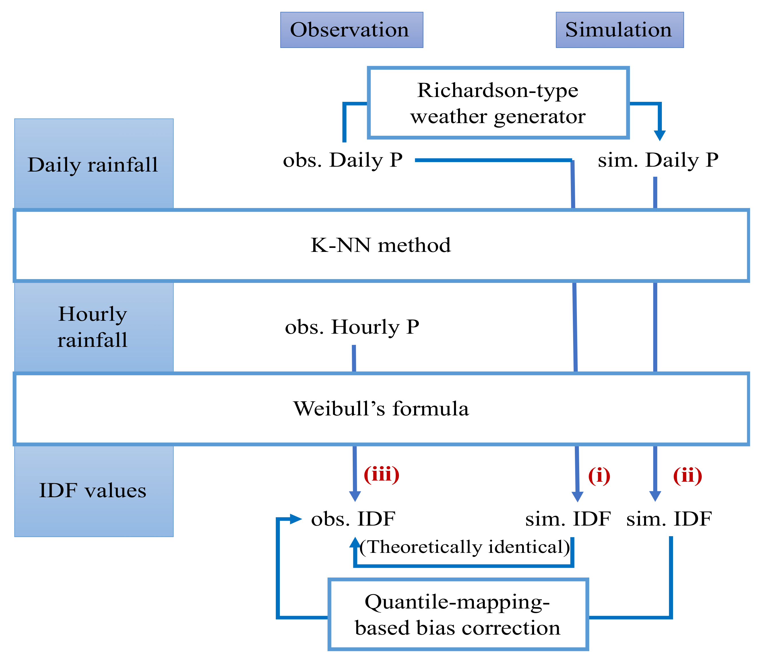
This study applies a Richardson-type weather generator [14] to generate daily rainfall, and then uses the k-NN method as a temporal downscaling method [36] for disaggregating the generated daily rainfall into hourly rainfall for selected stations across Taiwan. The occurrence of daily rainfall is generated by the weather generation model by assuming unchanged monthly characteristics, namely the probability of wet days (P(W)) for the first day of each month, and probabilities of wet days conditional on the previous wet (P(W|W)) or dry (P(W|D)) day for the rest of the month. If a uniform random number is smaller than these probabilities, a wet day is generated. The amounts of daily rainfall are generated randomly from the statistical distribution to which the historical daily rainfall data fits. For future projections, the original parameters of the statistical distribution are multiplied by the BCSD ratios of changes in precipitation for each scenario. Based on the assumption of the k-NN method, the hourly ratios of the most alike observed rainfall event concerning the daily rainfall amounts is extracted. When consecutive rainfall events were not found historically, remedy is provided in this study by combining historical events with different length in the same month as references (referring to Section 2.3). The hourly rainfall is used to derive the annual maximum series (AMS) and rainfall intensities for different return periods and durations based on the empirical Weibull method [54]. By Weibull’s formula, the corresponding return periods can be estimated using n (the total number of years in AMS) +1 dividing by m (rank = 1 represents the largest rainfall amounts in AMS). Since the relationship between the GCM simulation and observation is usually biased, the analysis results should undergo a bias correction step [53]. In case significant deviations occurs due to the limitation of the k-NN method in reproducing the randomness of hourly rainfall, this study employs a quantile mapping method [46] that corrects values of the annual maximum series according to the identified discrepancy between the empirical cumulative distribution function (ECDF) of the historical model run and that of the observed data (Figure 2). The procedure for rainfall projection is shown in Table 2. Details of the parameters used are introduced in Section 2.3.
2.3. Algorithm of the k-NN Method Used in the Study
The k-NN method is used to downscale the daily rainfall series to hourly in this study. The calculation of the k-NN method starts from the day when the rainfall amount of that day is greater than zero. By recording the consecutive rainy days (counting as n), the n-day rainfall events are recognized and compared with the rainfall events with the same length (n-day) in the pool of the historical events. Because there is limited information regarding the hourly ratios of rainfall in future scenarios, the stationary assumption is applied. That is, the hourly rainfall distribution ratio of a future rainfall event is assumed to be that of a historical event showing the daily rainfall amount closest to the generated event [36].
In the k-NN method, the distance dp between the observed and the generated consecutive n-day rainfall event is estimated using Equation (1). To determine the weights wt in Equation (1), while optimization methods can be used, this study adopts the reciprocal of the variance as the weights to estimate the distance with neighbors, as shown in Equation (2) [36]. The reciprocals of the variances are used as weights to allow more flexibility in selecting the most-alike historical events for the originally existed large variation of the nth day rainfall amount:
where gt is the generated daily rainfall on the tth day of the consecutive n-day event; ot,p is the observed daily rainfall on the tth day of the pth historical event in the pool with a total of f events; wt are the weights. Notice that the events in the pool are extracted from the defined window period. In this study, the month of the generated daily rainfall is chosen as the window period.
The window indicates a temporal period from which the observed n-day rainy events used to compare with the generated n-day rainy events are identified. In some studies, the window is set to be two weeks [5,36], while others investigate the optimal window size based on the observation [37,38]. In the study of Gunawardhana et al. [38], the performance is the best when the window size is between 28 and 40 days. Following the latter approach, the window of this study is set as one month.
The square root of the number of the potential neighbors is usually used for selecting k nearest neighbors [36], yet some studies suggested k smaller than 20 [55]. Similar to other studies that select one of the neighbors [5], the nearest neighbor is used to distribute hourly rainfall in this study to avoid smoothing the extremes caused by combining several historical rainfall events. The event with the smallest value of dp with rank one (r = 1), is selected. The hourly rainfall hq,t′ is determined by Equation (3), and the ratio of rainfall amount for each hour () is derived from the selected observed event:
where hq,t’ represents hourly rainfall simulated for the qth hour on the tth day; ot,r = 1 is the total rainfall amount of the tth day of the observations; and hq,t is the hourly rainfall for the qth hour on the tth day from the observations. Here the observations refer to the nearest observed neighboring n-day rainfall event.
Several realizations of the generated rainfall intensities, at least three times of the periods of record, are necessary to account for the uncertainty for future rainfall projections [36]. The study generates ten times (200 years) hourly rainfall of for each scenario. The configuration of the k-NN parameters used in this study is summarized in Table 3.
Randomness exists in the k-NN method because there may be many or no observed rainfall events which are like the generated event for downscaling. However, randomness increases for consecutive rainfall events that were not found historically, which is the limitation of k-NN method in considering the rainfall characteristics in the past. In this case, this study combines historical events with different length in the same month as references. For instance, if there are seven-day and nine-day events in May historically but no eight-day events we set m = 8. Previous studies that applied the k-NN method to hourly rainfall generation showed no explicit resolution of this issue [5,36,37,38,39], when no consecutive n-day rainfall events on record is generated through the use of the weather generator. Remedy is therefore provided in this study to generate hourly rainfall, by combining the historical events with the other rainfall events on record. The other historical rainfall events are determined based on the maximal length of consecutive rainy-day events Dmax in the same month. Afterwards, either one of the following two possible conditions is determined for the generation of future hourly rainfall, as shown in Equations (4) and (5):
- (1)
- If Dmax is larger than half of m, then the m-day is divided into two sets, namely a and b days (). All possible combinations of a and b are tried. After the m-day event is divided into new combinations, the distance dp (Equation (1)) of historical and simulated a- and b-day events are summed up as Equation (4). The optimal a and b are determined when the minimal distance is obtained:
- (2)
- If Dmax is smaller than half of m, Dmax is used to divide the m days as many times as possible. The m-day event becomes Dmax + … + Dmax + c, where c equals to m minus a multiple of Dmax. With the new combination, the distance dp (Equation (1)) of historical and simulated Dmax-day events are calculated as well as c-day events (m = ). When the minimal dp is obtained using Equation (5), the most alike multiple Dmax-day and c-day events are determined and used as references to generate future hourly rainfall for the m-day event:
3. Results and Discussion
The rainfall intensities of events with various duration and return periods are projected based on the generated hourly rainfall at the 21 weather stations in Taiwan under 10 (2RCP 5GCM) scenarios for the near-(2021–2040) and far-future (2081–2100). The short-duration and long-lasting extreme events are often of major concern in Taiwan as indicated in a previous study [12]. In this section, two types of events are focused on first, namely 1-h rainfall events in the 2-yr return period (eventsshort) and 24-h events in the 25-yr return period (eventslong), to examine the variation among locations and scenarios. Next, the influences of return periods and durations on rainfall intensities are analyzed.
Before further analysis, the verification of the k-NN method is addressed. By applying the proposed method to: (i) historically observed daily rainfall data, the IDF curves derived by the downscaled hourly rainfall data are the same as that by (iii) the observed hourly rainfall data. It shows the capability of the k-NN method to extract the hourly ratios of the most alike observed rainfall event and the thus verifies the reliability of the method, referring the relation between (i), (ii) and (iii) to Figure 2.
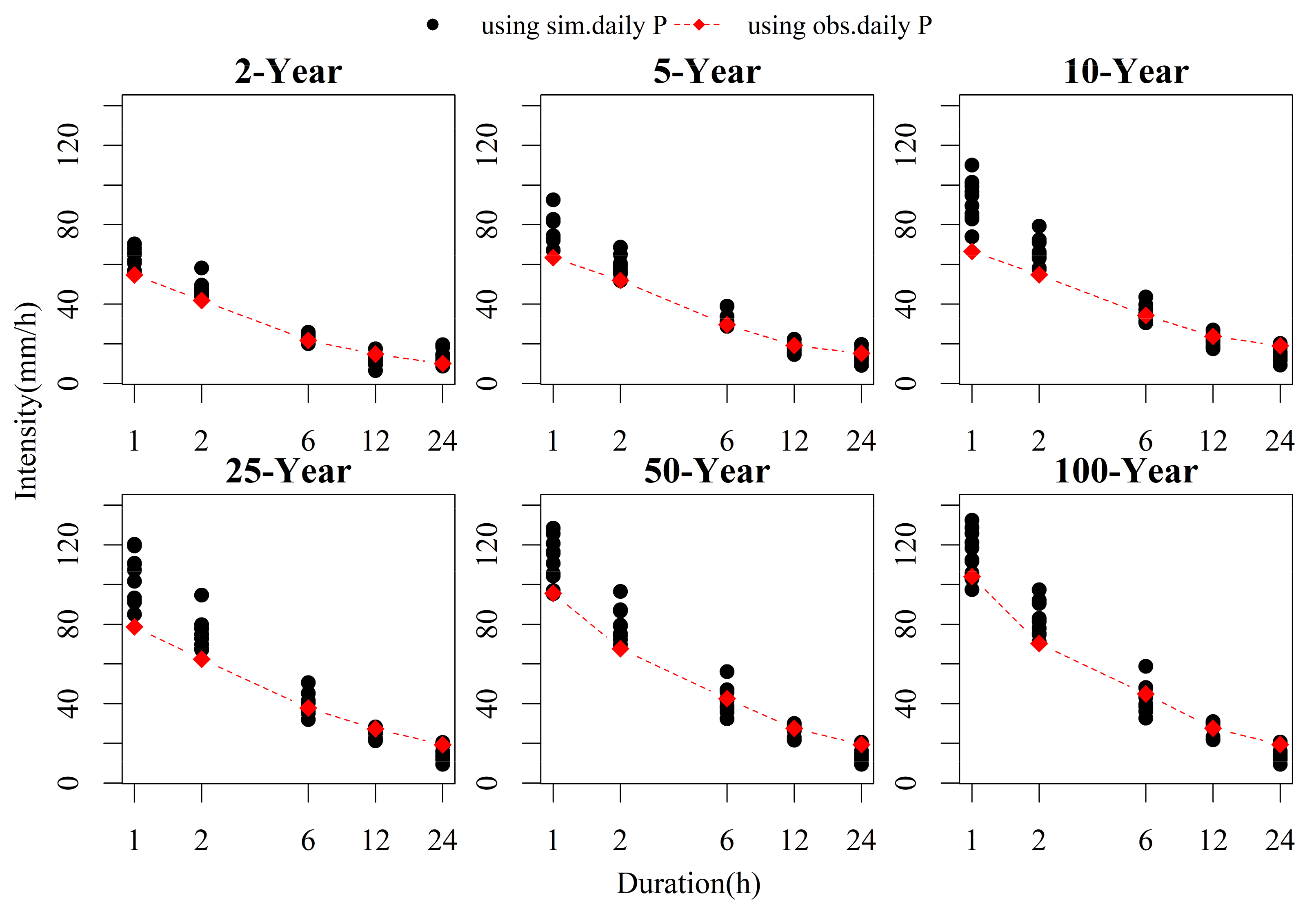
Considering there is noway to observe the daily rainfall in the future, it is projected. To further validate the applicability of the downscaling method for projected rainfall, the IDF curves derived from the k-NN method using both: (i) the simulated and (ii) the observed daily precipitation (denoted as ‘sim. daily P’ and ‘obs. daily P’) in the historical period (1986–2005) are compared. In fact, the k-NN method can capture the rainfall characteristics in some cases even before bias correction, e.g., Tainan case shown in Figure 3. The study generates ten times (200 years) daily rainfall based on Richardson-type weather generator, so there are ten realization of IDF values as shown in black dots (using (ii) sim. Daily P).
Deviations are found for some weather stations due to the limitation of the k-NN method; therefore, the study applies quantile-mapping-based bias correction to clearly present the values and changes of IDF curves. For certain duration, IDF from the 200-year data in total considering the ten black dots (using sim. Daily P) for the six return periods in Figure 3 comprise of the empirical cumulative distribution function (ECDF) of the historical annual maximum series and the values are corrected to (iii) the red diamonds (IDF using obs. Daily P) using the change factors. The same change factors are applied to the projected IDF values for the future periods.
3.1. Rainfall Variation among Locations and Scenarios
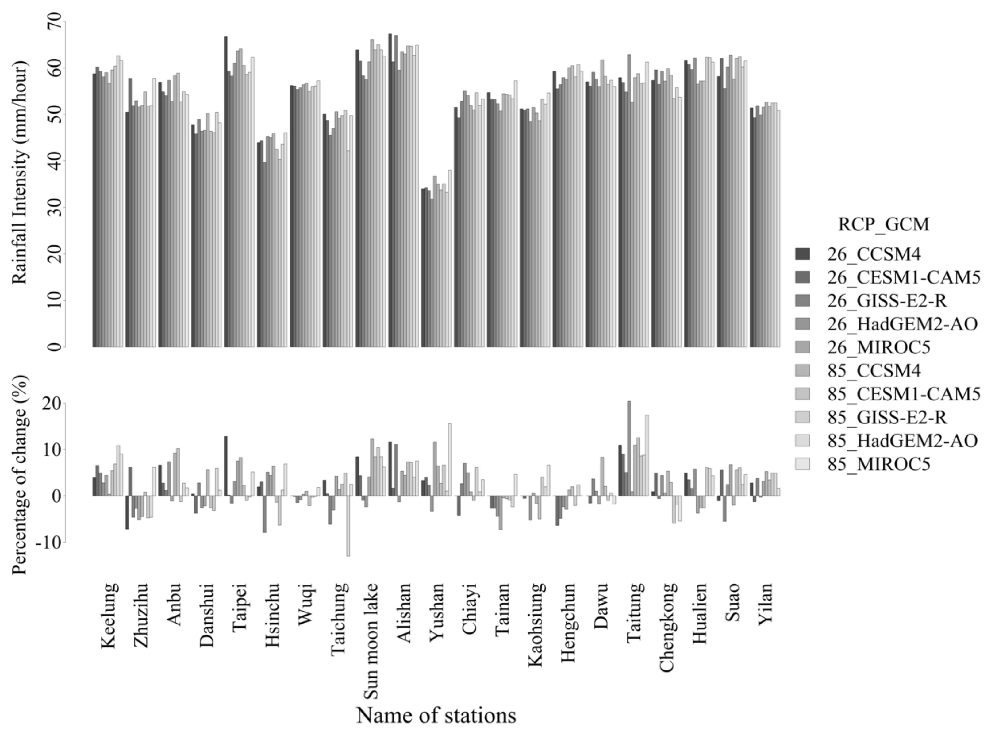
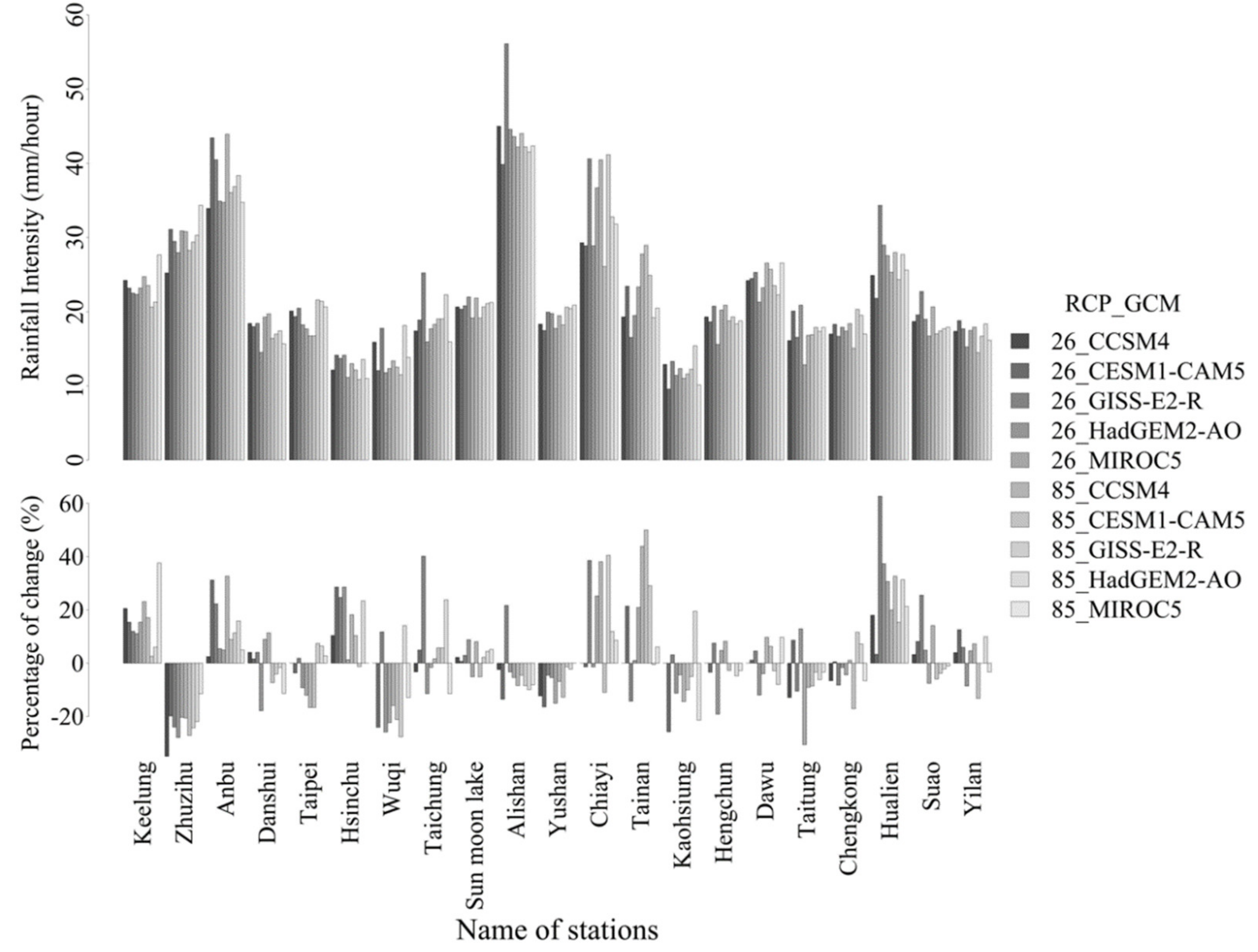
The rainfall intensities for eventsshort for the near- and far-future are depicted in Figure 4 and Figure 5, respectively. Both the rainfall intensities and the percentage changes compared to the observation in 1986–2005 are illustrated. The projected rainfall intensity of eventsshort is about 30–65 mm/h in the near future (Figure 4), while a slight increase is found for the far future (Figure 5). It is found that the variation of rainfall intensities among the locations is larger than that among the scenarios. After converting to change percentages, the variations among the scenarios become equally prominent, indicating deviation of the future rainfall intensities from the past. The projected rainfall-intensity changes of −10~20% were found in the near and far future. Comparing the results of RCP 2.6 and 8.5, opposite signs which show obvious difference between the two scenarios are found at Kaohsiung (− to +), Hengchun (− to +), and Chenggong (+ to −). Changes are intensified under RCP 8.5 for most other stations, except for Zhuzihu, Taipei, Hsinchu and Alishan, although no obvious difference are found for the two scenarios.
The variation of the rainfall intensities among the locations in northern and central Taiwan are larger than that in southern and eastern Taiwan. The reason is that in northern Taiwan, the Taoyuan Tableland lies in middle and in central Taiwan the altitude of the stations from mountain to coast results in different precipitation amounts. Notice that Yushan station in central Taiwan with altitude about 4000 m has less precipitation than Sun Moon Lake and Alishan, which is also observed in historical rainfall intensity of eventsshort. It is because the ventilation is good, and the height exceeds the zone where moisture is condensed. On the other hand, the altitudes and weather conditions of the stations are more even in southern and eastern Taiwan.
For most locations, there are both positive and negative changes projected in the near future, which is often occurred when using multiple models [37,46,55]. The exception are those locations that are always have plenty precipitation, including Keelung and Yilan in the northeastern part of Taiwan and Sun Moon Lake, Alishan, and Yushan in the mountainous area. The projected changes of these locations are mostly positive. The positive percentages of changes in Taitung are obvious compared to other stations, which is attributed to small values of observation. The precipitation of Taitung mainly comes from typhoon rain, but often the influence of typhoon on Taitung is not strong because the Central Mountains Range lies upwind of Taitung.
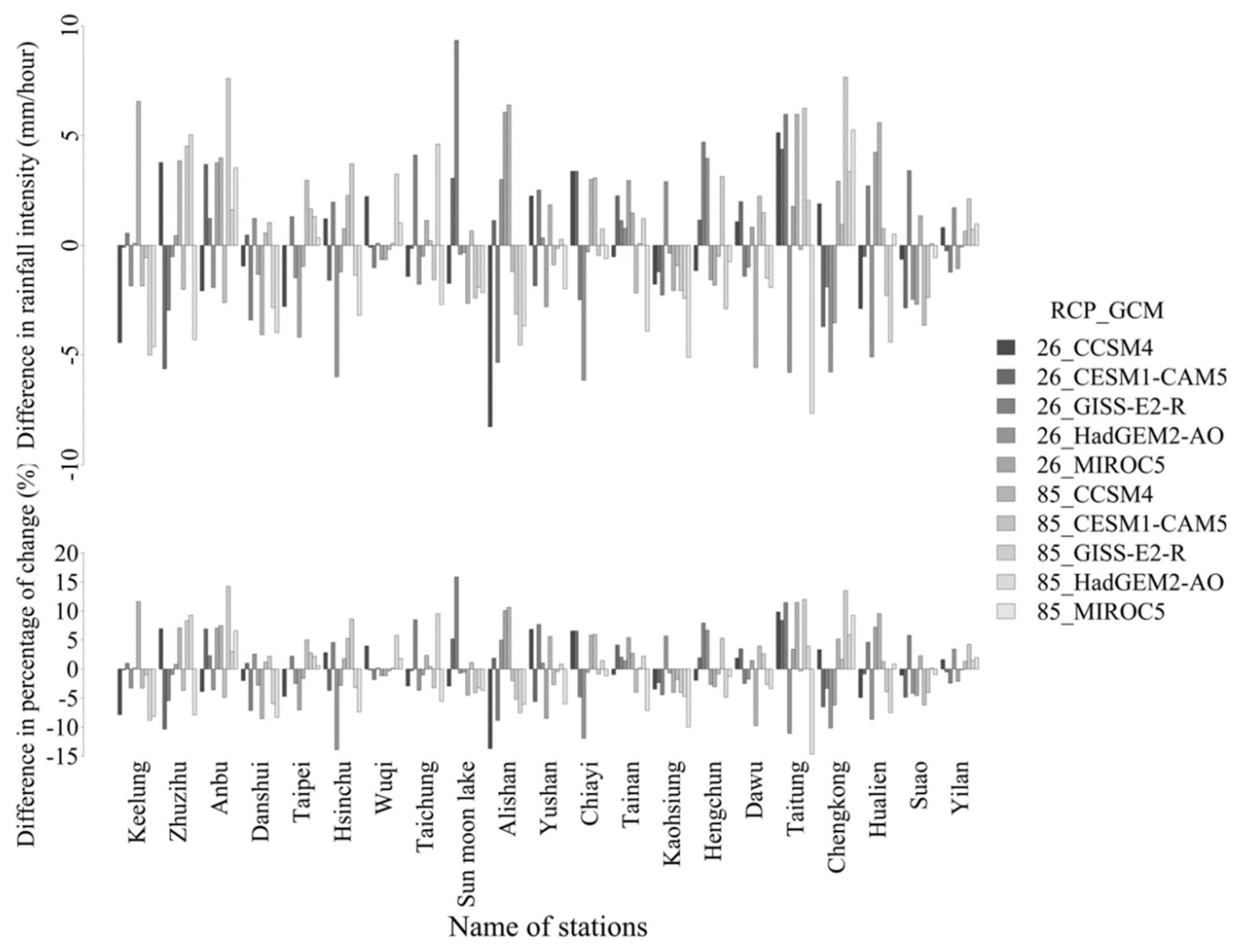
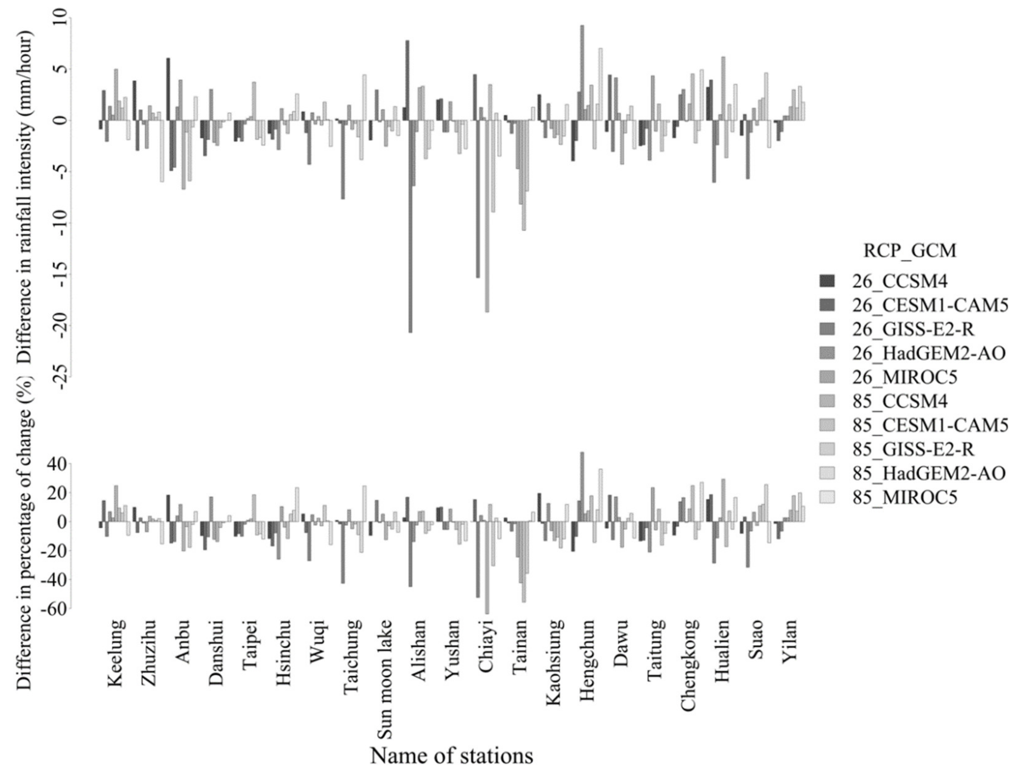
Figure 6 shows the difference between the near-(Figure 4) and far-future (Figure 5). It is found that the changes of the projected rainfall intensities between the two periods vary with the scenarios. The uncertainty exists, which influences the robustness of the decision related to pluvial flooding as suggested by the result. Previous studies also showed larger differences between GCMs for the far-future projections compared to the near-future especially for short-duration or large-return-period events [37,38]. For certain stations at least 80% of the scenarios agree on the decrease in the rainfall intensities in the far future compared to the near future, including Keelung, Kaohsiung, and Suao. Although only 60% of the scenarios agree on the decrease, Danshui also shows a decreasing trend considering the projected rainfall intensities. The existing drainage capacities for cities in Taiwan are based on different protecting levels. For instance, the hourly rainfall intensity thresholds for flood warning at Keelung, Danshui, Kaohsiung, and Suao are 50, 60, 70 and 70 mm, while the historical extreme rainfall intensities per hour after 1986 are 95 mm (31 August 2013), 107.5 mm (2 June 2017), 119.5 mm (11 July 2001) and 181.5 mm (21 October 2010), respectively. The extreme events may be caused by the plum rains, southwesterly flows, or typhoons. Considering that these places may be vulnerable to flooding, precautions should still be taken for the frequently occurred short-duration storm events despite of decreasing in projection for the two periods.
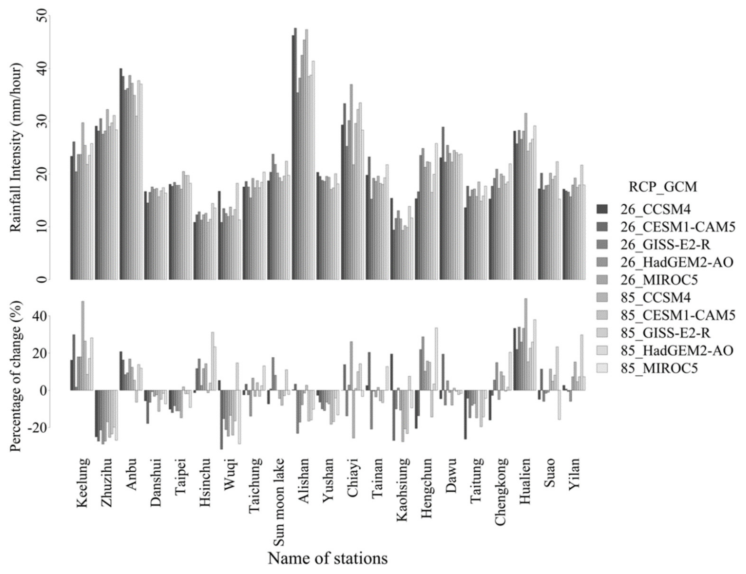
Likewise, the rainfall intensities of eventslong for the near and far-future are depicted in Figure 7 and Figure 8, respectively.
For a longer duration and a larger return period, both the variations among the scenarios and among the stations increase. In the near future, the rainfall intensities are between 12 and 45 mm per hour, which equals to 288–1080 mm per day.
Compared to the historical period, Zhuzihu, Wuqi, Alishan, Yushan, Kaohsiung and Taitung show decreasing intensities, while Keelung, Anbu, Hsinchu, Chiayi, Tainan, and Hualien show increasing intensities. The remaining stations show less obvious changes. The 24-h/daily rainfall intensity thresholds for flood warning at Zhuzihu, Wuqi, Alishan, Yushan, Kaohsiung, and Taitung are 350, 350, 450, 400, 350 and 400 mm, while at Keelung, Anbu, Hsinchu, Chiayi, Tainan and Hualien are 300, 350, 300, 300, 300, 300 mm, respectively. Our projection results show that only Wuqi, Hsinchu, and Kaohsiung are found equal to or smaller than the flood warning thresholds.
The changes in the projected long-duration rainfall intensities from the near- to far-future show large uncertainty among the scenarios (Figure 9). For Danshui, Tainan, and Taitung stations showing more prominent changes, we can find that at least 80% of the scenarios agree on the direction of changes. If near no-change scenarios are excluded, the decreasing intensities are found for Danshui, Taipei, Taichung, Tainan and Taitung, while the increasing intensities are found for Yilan. It seems that the rainfall intensities decrease mostly from the near- to far-future, which is more obvious for eventslong compared to eventsshort. For future studies, events with longer return periods than 25-yr return periods should better be analyzed using record of the observed data longer than 20 years to disclose more information.
The current engineering design of drainage systems in Taiwan exhibits the capacity to drain extreme stormwater to a certain extent; however, the extreme events have become more frequently and stronger since the 1980s. The rainfall amounts of the top five historical events in Taiwan were 1748.5 mm/day at Alishan (1996), 1151.9 at Zhuzihu (1987), 1018.5 at Suao (2010), 879.3 at Yushan (2009), and 871 at Chiayi (2001). These extreme events with a long duration induced severe compound disasters including landslides and mudflows. Moreover, the local projection could considerably exceed the GCM projection, based on another dynamical downscaling study [56]. Since the projected rainfall is greater than the flood-warning threshold, the risk of pluvial flooding is still substantial under climate change scenarios. Among all stations, the land-subsidence region such as Chiayi (in central) and potentially Tainan (in south), the landslide-sensitive region such as Zhuzihu and Anbu in the north and Alishan and Yushan in the central, the pluvial- and fluvial-flood prone region such as Keelung (in north), and the regions with vulnerable infrastructures such as Hualien and Taitung (in east) should be especially aware of long-duration extreme events.
3.2. Association between Return Periods/Durations and Rainfall Intensities
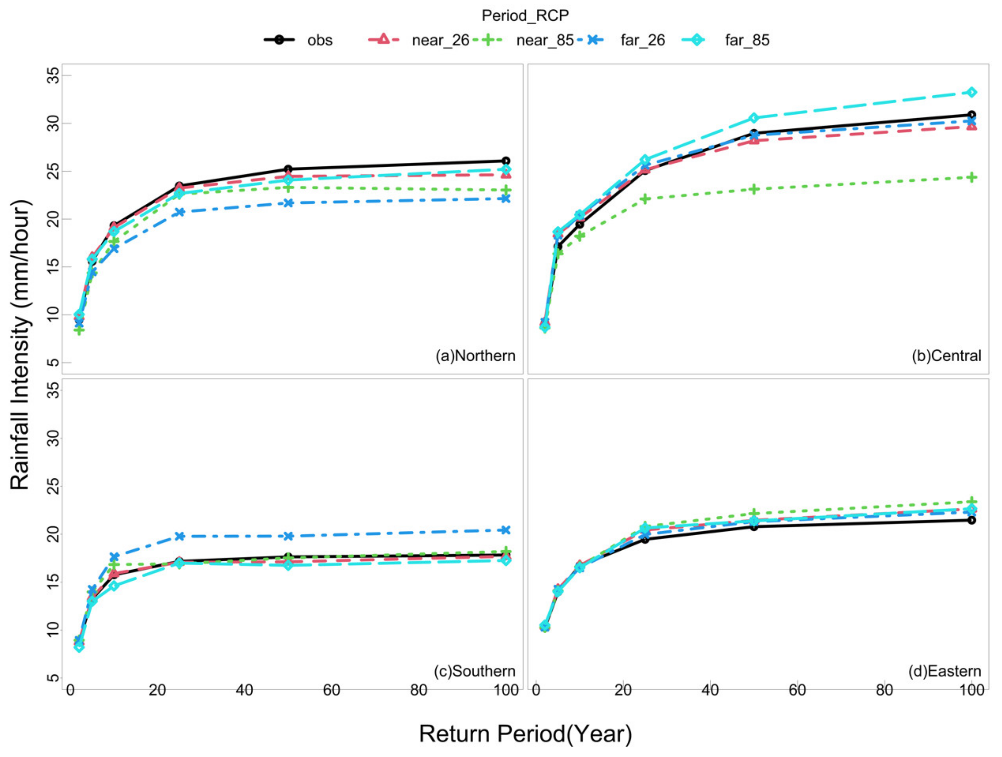
Apart from events with given durations and return periods, the association of these two parameters with rainfall intensities is further investigated. Firstly, the duration is fixed, and then rainfall intensities are plotted against different return periods (Figure 10 and Figure 11); similarly, results by fixing the return period are also derived (Figure 12 and Figure 13). To reduce the complexity of the figures, regional results are derived from averaging station data in the four major regions, and the scenarios are categorized into near_26, near_85, far_26, and far_85, representing the near/far-future under RCP 2.6/8.5.
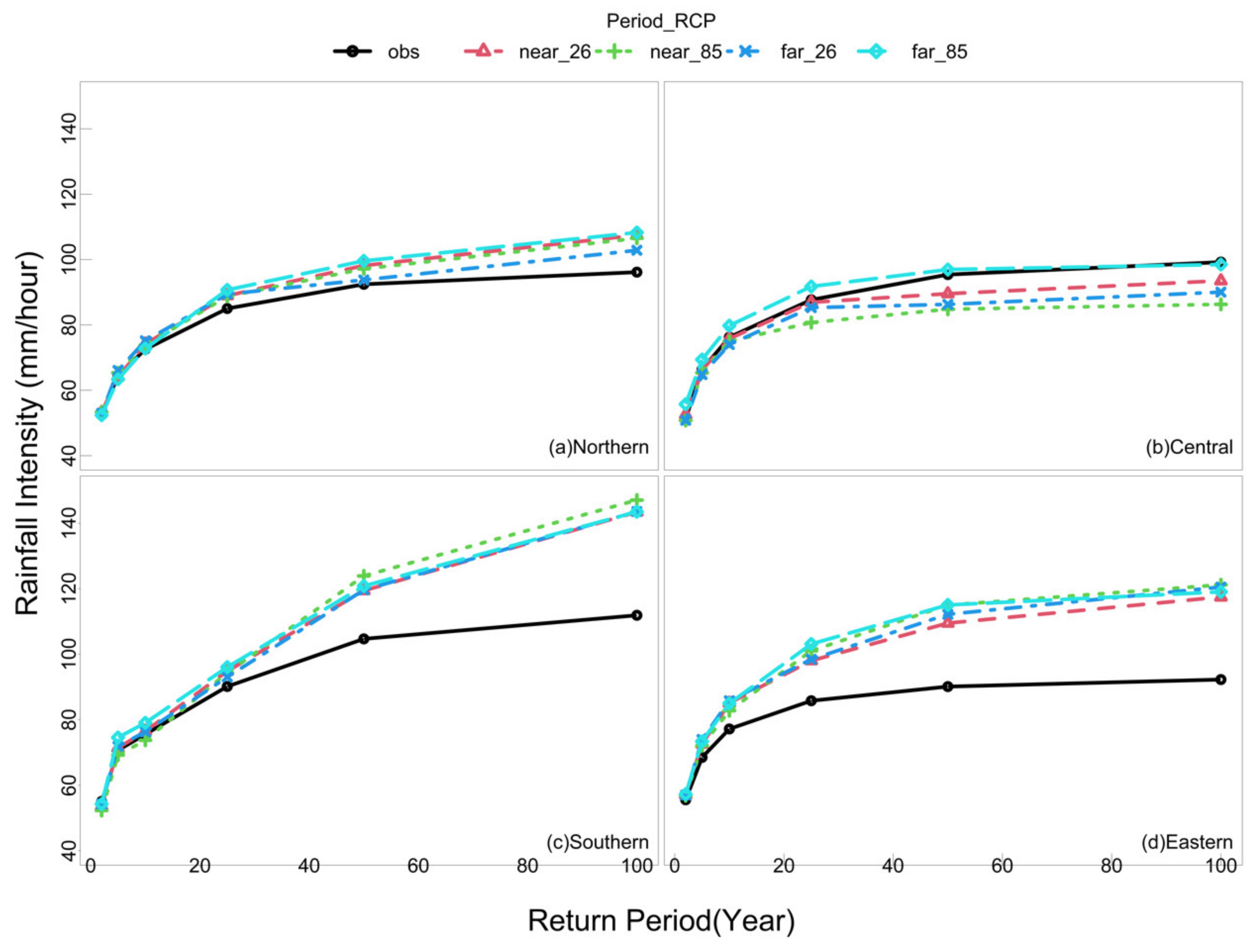
Figure 10 shows the intensity-frequency curves (i.e., intensities vs. return periods) for the four regions and four scenarios. The duration is fixed at one hour, so associated events are hereafter denoted as D1 events. Rainfall intensities increase as frequencies decrease. However, for some frequencies it is found that the changes of the four scenarios from observation are similar. These frequencies include the return periods shorter than 25 years for the northern region, that shorter than two years in southern region, and that shorter than ten years in eastern region. For smaller frequencies (larger return periods) than these frequencies, the uncertainty brought by the scenarios shows the interval about 5 mm/h in the northern, southern, and eastern regions, while the interval in the central region is about three times larger. Alishan and Chiayi stations in the central region are the main reason of the variation among the scenarios. More hourly precipitation records larger than 110 mm are found in the two stations compared to the other stations, which increase the probability of larger hourly rainfall being selected from the historical events during the k-NN temporal downscaling process.
Figure 10 also indicates that the central region has decreased extreme rainfall intensities from the observation in the future, which is opposite from the other regions. More specifically, the intensities of the 2-yr return period in all the regions barely show differences, while that of the 100-yr return period are about 110, 90, 150, 120 mm/h in the northern, central, southern, and eastern regions. These results are influenced by the ratios based on BCSD data of the GCMs projection under different scenarios, which are about 0–10%, –10–0%, 0–30% and 0–30%, respectively, in the northern, central, southern, and eastern regions from the 2-yr to 100-yr return periods. For the 50 and 100-yr return periods, the projections of the southern region are the largest among the regions, while that in the eastern region are more prominent than the other regions for the return periods of 25 years. According to the above results, events with the return periods of 10 and 25 years in the eastern region and that of 50 and 100 years in the southern region that differ a lot from the past experiences should be of concern, and adaptation measures such as establishing distributed drainage system or renewing hydrological infrastructures to ensure the resilience to extreme events are suggested.
Figure 11 shows the intensity-frequency curves for the 24-h (D24) events. The uncertainty brought by the scenarios shows the largest interval in the central region, followed by the northern, southern, and eastern regions. Large uncertainty in the central region can be found especially for the high return periods (50 and 100 years). For the return periods larger than 10 years, the results show much smaller intensities projected for the northern region than observation, a bit larger for the eastern region, and relatively ambiguous direction of changes for far future for central and southern regions where one of the scenarios deviated from the others. Considering the uncertainty caused by time, the projections of near future should take precedence over the far-future scenarios and adaptation addressing the increasing intensities in the eastern region is recommended. For far future, adaptations are also suggested in the central and southern regions against the increasing rainfall intensities.
The main cause of short-duration storm events (D1) are plum rains, southwesterly flows, and convective rain, while that of long-duration events (D24) are typhoon rains and northeasterly monsoon. It explains the projected results of D1 and D24 in Figure 10 and Figure 11. The extreme D1 and D24 events with large return periods are mainly from southwesterly flows and typhoon rains, so southern and eastern region (especially Taitung in the south east) show more prominent increase in intensities. The results are consistent to the projections in the scientific report of Taiwan that precipitation in summer increases in the future [49]. Also, a decrease of precipitation from the northeasterly monsoon was found in the report [49].
This is probably the reason that decreased rainfall intensities are projected in the northern region, where the precipitation relies heavily on the northeasterly monsoon. On the other hand, the projected changes are substantial for the eastern region for the D1 events, but quite minute for the D24. Because the precipitation from the northeasterly monsoon decreases, the increases of rainfall intensities of the long-duration events that influence the eastern region are minute. In addition, although the peak rainfall intensities of typhoons may increase, the average rainfall intensities of 24-h is not prominent.
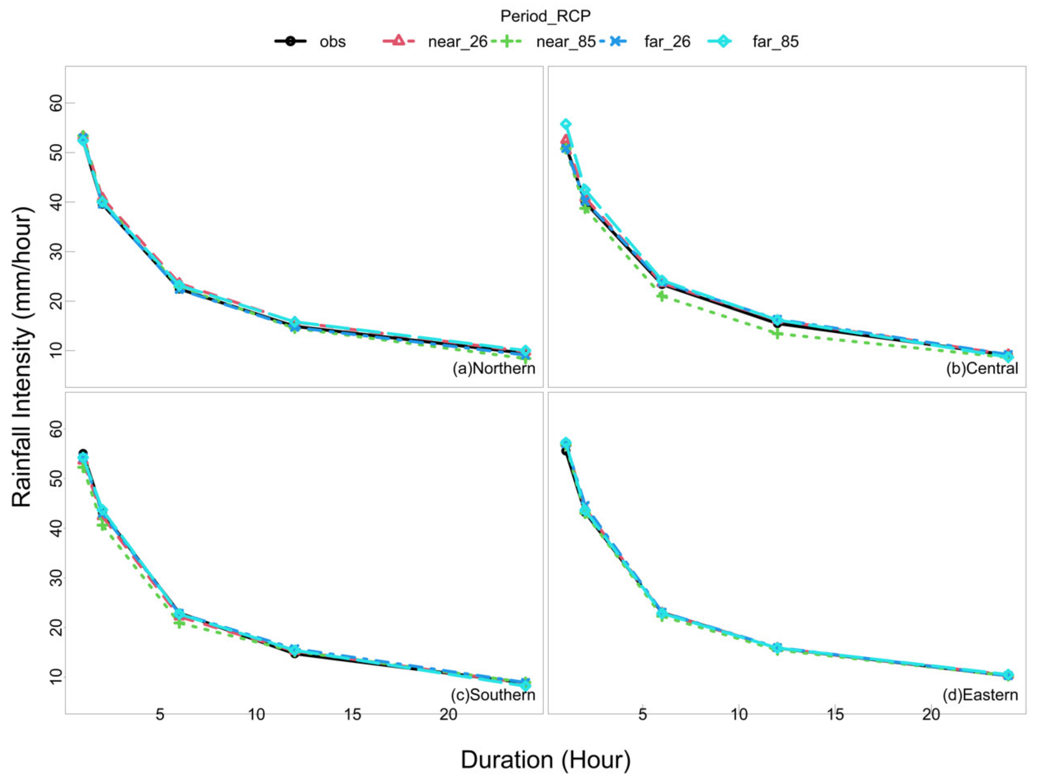
To examine the association between the rainfall intensity and duration, the intensity-duration curves derived from setting the return periods of the events as 2 (T2) and 25 years (T25) are shown in Figure 12 and Figure 13, respectively. Note that for T2, the probability of exceedance for an event in a year is 50%. In Figure 12, it is found that for all the regions the curves are nearly identical to the observation regardless of the scenarios, except that a slight decrease in the intensities of events with the 6 and 12-h durations in the central region under RCP 8.5 in the near future (near_85). The results indicate that the average rainfall intensities of events with different durations in the future are similar to the observation, compared to that with different return periods that are larger than 10-yr shown in Figure 10 and Figure 11.
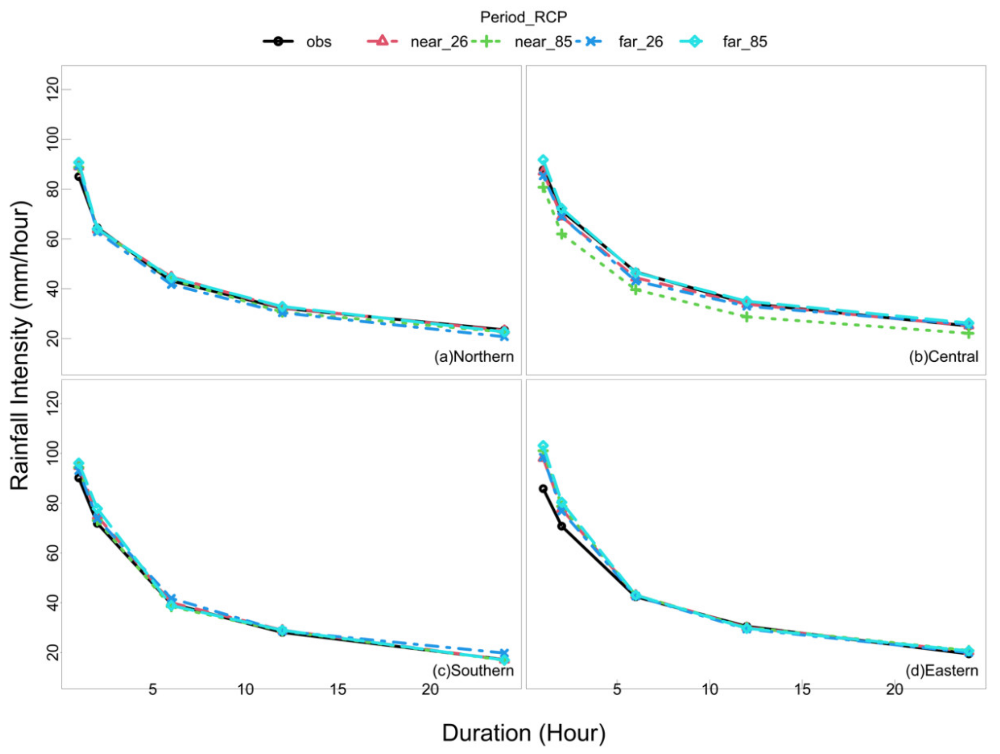
The intensity-duration curves for the T25 events also show a narrow uncertainty interval, except in the central region under the near_85 scenario (Figure 13) which shows a about 5 mm/h decrease for different durations. Considering future intensities deviate from the observation, little changes are identified for most scenarios; however, some exceptions exist. For 1-h-duration events, slight increases of the rainfall intensities are found in the northern and southern regions. Furthermore, 10–15 mm/h increases are shown for the 1 and 2-h durations in the eastern region. For 24-h-duration events, the projections of far_26 in the northern region and that of near_85 in the central region are smaller than observation, in addition to the aforementioned case of central region under the near_85 scenario.
Combining the information of D1, D24, T2 and T25 projections from Figure 10, Figure 11, Figure 12 and Figure 13, the rainfall characteristics in the four regions are further discussed. For events with smaller intensities (T2), the changes in the future are little which applies to the four regions, but for those with larger intensities (T25), the changes of 1 and 2-h-duration events are prominent in the eastern region, followed by the 1-h-duration events in the southern and the northern regions (Figure 12 and Figure 13). It is because these short-duration events have significant increases projected in the future in the southern and eastern regions, followed by northern region, compared to the long-duration events (Figure 9 and Figure 10). Moreover, it can be seen from Figure 10 that the BCSD ratio of T25 events are much larger in the eastern region than in the southern region. The results of the increases in rainfall intensities of short-duration extreme events are consistent to the projections in other regional and local studies [48,49].
This study provides information of changes in future rainfall intensities to assist adaptation-related decision-making. Based on the results, design storm analysis can be the next step, to assess hydrological responses to storm series for more detailed stormwater/water resource management. The hyetograph suitable for the target area can be analyzed using the Simple Scaling Gauss-Markov method that has been developed across Taiwan, if the normality and the correlation coefficients of the rainfall-event records fulfill the assumptions of the Gauss–Markov model [57]. Moreover, it is worth mentioning that here only the rainfall intensities of single events are analyzed rather than the effect of continuous rainfall events, which may cause severe disasters in Taiwan based on the past experiences. Therefore, further studies on these events are recommended and it is necessary to be alert although similar intensities are projected for long-duration events.
4. Conclusions
This study analyzed the changes in rainfall intensities in Taiwan and its association with different return periods and durations under climate change scenarios using the k-NN method. Daily rainfall was first generated by a Richardson-type weather generator, and then the k-NN method was used to disaggregate the daily rainfall to hourly rainfall that can thus be used for estimating rainfall intensities through an empirical Weibull formula. Finally, CDF-based bias correction was applied to events for different durations and return periods. The projections of the 21 weather stations in Taiwan under 10 (2RCP5GCM) scenarios for the near-(2021–2040) and far-future (2081–2100) were derived.
Changes in the rainfall intensities associated with the two types of events, namely events with 1-h duration and 2-yr return period (eventsshort) and with 24-h duration and 25-yr return period (eventslong), were discussed. For eventsshort, the projected rainfall-intensity changes of 10~20% were found under future scenarios compared to the observations. Considering the existing flood-warning thresholds, precautions of flooding are required for the frequently occurred short-duration storm events in Keelung, Danshui, Kaohsiung, and Suao, although rainfall intensities are projected to decrease from the near to the far future.
For eventslong, the majority of the projected rainfall intensities exceeded the flood-warning threshold despite of the decreasing intensities compared to observation, which should be of concern. Compared to eventsshort, the decreases in the rainfall intensities of eventslong are more obvious from near to far future. Among all stations, the land-subsidence regions in central and south, the landslide-sensitive mountainous region in north and central, the pluvial- and fluvial-flood prone region in north, and the regions with vulnerable infrastructures in east should be especially aware of possible long-duration extreme events. It should be noted that because the observed data has a period of record of 20 years, only the 25-yr return period are presented here; however, events with longer return periods than 25-yr return periods should better be analyzed to disclose more information of extreme events the cities face in the future.
Further, the association between the rainfall intensity and the return period, by controlling the duration, was analyzed. For events with the 1-h duration (D1), the percentage changes in the northern, central, southern, and eastern regions are about 0–10%, –10–0%, 0–30%, and 0–30%, respectively. The changes in the central region are the smallest, but the uncertainty among the scenarios are the largest. Moreover, events with the return periods of 10 and 25 years in the eastern region and that of 50 and 100 years in the southern region should be of concern, and adaptation measures such as establishing distributed drainage system or renewing hydrological infrastructures to ensure the resilience to extreme events are suggested.
For events with the 24-h duration (D24) and for the return periods larger than 10 years, the projected intensities are much smaller in the northern region, a bit larger in the eastern region, and probably larger in the central and southern regions for far future compared to the observation. Therefore, adaptation in the eastern region is suggested considering the near future projection, and in the central and the southern regions for far future, too. The projected results are caused mainly by the increased precipitation in summer and decreased precipitation from the northeasterly monsoon in future.
Similarly, the intensity-duration relationships were projected for the 2-yr (T2) and 25-yr (T25) return-period events. The results indicate that the average rainfall intensities of events with different durations in the future are similar to the observation, compared to that with different return periods that are larger than 10-yr. In short, the changes in the future are little which applies to the four regions for events with smaller intensities (T2), but the changes of 1 and 2-h-duration events are prominent in the eastern region, followed by the 1-h-duration events in the southern and the northern regions for those with larger intensities (T25).
To conclude, the short-duration extreme events are probably stronger than before. Moreover, places without experience of long-lasting events with rainfall amounts larger than 500 mm such as Keelung and Hualien should be alert. This study provides information regarding the changes in future rainfall intensities, which can be used to assist adaptation-related decision-making. Based on the results, design storm analysis can be one of the ensuing studies, to assess hydrological responses to storm series for more detailed stormwater/water resource management.
Author Contributions
Conceptualization and methodology, P.-Y.C. and C.-P.T.; software, P.-Y.C.; formal analysis, P.-Y.C., C.-P.T. and J.-H.T.; investigation, P.-Y.C., J.-H.T. and C.-J.C.; writing—original draft preparation, P.-Y.C. and C.-J.C.; writing—review and editing, J.-H.T. and C.-J.C. All authors have read and agreed to the published version of the manuscript.
Funding
This study and the APC are partially supported by Ministry of Science and Technology of Taiwan (MoST) under Contract No. 108-2313-B-008-001-MY3.
Data Availability Statement
Original ratios of changes in precipitation were obtained from National Science and Technology Center for Disaster Reduction (NCDR), Taiwan and are available https://tccip.ncdr.nat.gov.tw/ds_03_eng.aspx (24 May 2021) with the permission of NCDR.
Acknowledgments
This study is partially supported by the Ministry of Science and Technology of Taiwan (MoST) under Contract No. MOST 108-2313-B-008-001-MY3.
Conflicts of Interest
The authors declare no conflict of interest.
References
- Neumann, B.; Vafeidis, A.T.; Zimmermann, J.; Nicholls, R. Future Coastal Population Growth and Exposure to Sea-Level Rise and Coastal Flooding—A Global Assessment. PLoS ONE 2015, 10, e0118571. [Google Scholar] [CrossRef] [PubMed] [Green Version]
- Hughes, B.; Lowe, J.A.; Nicholls, R.; Osborn, T. The impacts of climate change across the globe: A multi-sectoral assessment. Clim. Chang. 2016, 134, 457–474. [Google Scholar]
- Nolan, P.; O’Sullivan, J.; McGrath, R. Impacts of climate change on mid-twenty-first-century rainfall in Ireland: A high-resolution regional climate model ensemble approach. Int. J. Climatol. 2017, 37, 4347–4363. [Google Scholar] [CrossRef]
- Cheng, L.; AghaKouchak, A. Nonstationary Precipitation Intensity-Duration-Frequency Curves for Infrastructure Design in a Changing Climate. Sci. Rep. 2015, 4, 7093. [Google Scholar] [CrossRef] [PubMed] [Green Version]
- Peck, A.; Prodanovic, P.; Simonovic, S.P.P. Rainfall Intensity Duration Frequency Curves Under Climate Change: City of London, Ontario, Canada. Can. Water Resour. J. Rev. Can. Des Ressour. Hydr. 2012, 37, 177–189. [Google Scholar] [CrossRef]
- De Paola, F.; Giugni, M.; Topa, M.E.; Bucchignani, E. Intensity-Duration-Frequency (IDF) rainfall curves, for data series and climate projection in African cities. Springer Plus 2014, 3, 1–18. [Google Scholar] [CrossRef] [Green Version]
- Olesen, J.E.; Trnka, M.; Kersebaum, K.; Skjelvåg, A.; Seguin, B.; Peltonen-Sainio, P.; Rossi, F.; Kozyra, J.; Micale, F. Impacts and adaptation of European crop production systems to climate change. Eur. J. Agron. 2011, 34, 96–112. [Google Scholar] [CrossRef]
- Arnell, N.W.; Lloyd-Hughes, B. The global-scale impacts of climate change on water resources and flooding under new climate and socio-economic scenarios. Clim. Chang. 2014, 122, 127–140. [Google Scholar] [CrossRef] [Green Version]
- Li, C.-Y.; Lin, S.-S.; Chuang, C.-M.; Hu, Y.-L. Assessing future rainfall uncertainties of climate change in Taiwan with a bootstrapped neural network-based downscaling model. Water Environ. J. 2018, 34, 77–92. [Google Scholar] [CrossRef]
- Huang, W.; Chang, Y.; Hsu, H.; Cheng, C.; Tu, C. Dynamical downscaling simulation and future projection of summer rainfall in Taiwan: Contributions from different types of rain events. J. Geophys. Res. Atmos. 2016, 121, 13–973. [Google Scholar] [CrossRef]
- Wei, C.; Yeh, H.; Chen, Y.; Cheng, K. Stochastic simulation for design storm with different return periods and du-rations, annual and monthly rainfall of the National Taiwan University Experimental Forest. J. Exp. For. Natl. Taiwan Univ. 2016, 30, 153–176. [Google Scholar]
- Chen, C.W.; Tung, Y.S.; Liou, J.J.; Li, H.C.; Cheng, C.T.; Chen, Y.M.; Oguchi, T. Assessing landslide characteris-tics in a changing climate in northern Taiwan. Catena 2019, 175, 263–277. [Google Scholar] [CrossRef]
- Chen, Y.M.; Chen, C.W.; Chao, Y.C.; Tung, Y.S.; Liou, J.J.; Li, H.C.; Cheng, C.T. Future Landslide Characteris-tic Assessment Using Ensemble Climate Change Scenarios: A Case Study in Taiwan. Water 2020, 12, 564. [Google Scholar]
- Richardson, C.W. Stochastic simulation of daily precipitation, temperature, and solar radiation. Water Resour. Res. 1981, 17, 182–190. [Google Scholar] [CrossRef]
- Semenov, M.A.; Barrow, E.M.; Lars-Wg, A. A Stochastic Weather Generator for Use in Climate Impact Studies; User Manual: Hertfordshire, UK, 2002. [Google Scholar]
- Mailhot, A.; Duchesne, S.; Caya, D.; Talbot, G. Assessment of future change in intensity–duration–frequency (IDF) curves for Southern Quebec using the Canadian Regional Climate Model (CRCM). J. Hydrol. 2007, 347, 197–210. [Google Scholar] [CrossRef]
- DeGaetano, A.T.; Castellano, C.M. Future projections of extreme precipitation intensity-duration-frequency curves for climate adaptation planning in New York State. Clim. Serv. 2017, 5, 23–35. [Google Scholar] [CrossRef]
- Cook, L.M.; McGinnis, S.; Samaras, C. The effect of modeling choices on updating intensity-duration-frequency curves and stormwater infrastructure designs for climate change. Clim. Chang. 2020, 159, 289–308. [Google Scholar] [CrossRef] [Green Version]
- Rasmussen, S.B.; Blenkinsop, S.; Burton, A.; Abrahamsen, P.; Holm, P.E.; Hansen, S. Climate change impacts on agro-climatic indices derived from downscaled weather generator scenarios for eastern Denmark. Eur. J. Agron. 2018, 101, 222–238. [Google Scholar] [CrossRef]
- So, B.-J.; Kim, J.-Y.; Kwon, H.-H.; Lima, C.H. Stochastic extreme downscaling model for an assessment of changes in rainfall intensity-duration-frequency curves over South Korea using multiple regional climate models. J. Hydrol. 2017, 553, 321–337. [Google Scholar] [CrossRef]
- Hassanzadeh, E.; Nazemi, A.; Elshorbagy, A. Quantile-based downscaling of precipitation using genetic program-ming: Application to IDF curves in Saskatoon. J. Hydrol. Eng. 2014, 19, 943–955. [Google Scholar] [CrossRef]
- Mirhosseini, G.; Srivastava, P.; Fang, X. Developing Rainfall Intensity-Duration-Frequency Curves for Alabama under Future Climate Scenarios Using Artificial Neural Networks. J. Hydrol. Eng. 2014, 19, 04014022. [Google Scholar] [CrossRef]
- Ivanov, V.Y.; Bras, R.L.; Curtis, D.C. A weather generator for hydrological, ecological, and agricultural applications. Water Resour. Res. 2007, 43. [Google Scholar] [CrossRef] [Green Version]
- Peleg, N.; Molnar, P.; Burlando, P.; Fatichi, S. Exploring stochastic climate uncertainty in space and time using a gridded hourly weather generator. J. Hydrol. 2019, 571, 627–641. [Google Scholar] [CrossRef]
- Müller, H.; Haberlandt, U. Temporal rainfall disaggregation with a cascade model: From single-station disaggrega-tion to spatial rainfall. J. Hydrol. Eng. 2015, 20, 04015026. [Google Scholar] [CrossRef] [Green Version]
- De Luca, D.L. Analysis and modelling of rainfall fields at different resolutions in southern Italy. Hydrol. Sci. J. 2014, 59, 1536–1558. [Google Scholar] [CrossRef] [Green Version]
- Menabde, M.; Sivapalan, M. Modeling of rainfall time series and extremes using bounded random cascades and levy-stable distributions. Water Resour. Res. 2000, 36, 3293–3300. [Google Scholar] [CrossRef] [Green Version]
- Over, T.M.; Gupta, V.K. Statistical Analysis of Mesoscale Rainfall: Dependence of a Random Cascade Generator on Large-Scale Forcing. J. Appl. Meteorol. 1994, 33, 1526–1542. [Google Scholar] [CrossRef] [Green Version]
- Choi, J.; Lee, O.; Jang, J.; Jang, S.; Kim, S. Future intensity–depth–frequency curves estimation in Korea under rep-resentative concentration pathway scenarios of Fifth assessment report using scale-invariance method. Int. J. Climatol. 2019, 39, 887–900. [Google Scholar] [CrossRef]
- Cannon, A.J.; Innocenti, S. Projected intensification of sub-daily and daily rainfall extremes in convec-tion-permitting climate model simulations over North America: Implications for future intensity–duration–frequency curves. Nat. Hazards Earth Syst. Sci. 2019, 19, 421–440. [Google Scholar] [CrossRef] [Green Version]
- Yang, X.; He, R.; Ye, J.; Tan, M.L.; Ji, X.; Tan, L.; Wang, G. Integrating an hourly weather generator with an hourly rainfall SWAT model for climate change impact assessment in the Ru River Basin, China. Atmos. Res. 2020, 244, 105062. [Google Scholar] [CrossRef]
- Peleg, N.; Fatichi, S.; Paschalis, A.; Molnar, P.; Burlando, P. An advanced stochastic weather generator for simu-lating 2-D high-resolution climate variables. J. Adv. Modeling Earth Syst. 2017, 9, 1595–1627. [Google Scholar] [CrossRef]
- Blenkinsop, S.; Harpham, C.; Burton, A.; Goderniaux, P.; Brouyère, S.; Fowler, H.; Fowler, H. Downscaling transient climate change with a stochastic weather generator for the Geer catchment, Belgium. Clim. Res. 2013, 57, 95–109. [Google Scholar] [CrossRef] [Green Version]
- Burton, A.; Fowler, H.; Blenkinsop, S.; Kilsby, C. Downscaling transient climate change using a Neyman–Scott Rectangular Pulses stochastic rainfall model. J. Hydrol. 2010, 381, 18–32. [Google Scholar] [CrossRef]
- De Luca, D.; Petroselli, A.; Galasso, L. A Transient Stochastic Rainfall Generator for Climate Changes Analysis at Hydrological Scales in Central Italy. Atmosphere 2020, 11, 1292. [Google Scholar] [CrossRef]
- Solaiman, T.A.; Simonovic, S.P. Development of Probability Based Intensity-Duration-Frequency Curves under Climate Change. Water Resour Res Rep. 2011, 34, 1–93. [Google Scholar]
- Alam, M.S.; Elshorbagy, A. Quantification of the climate change-induced variations in Intensity–Duration–Frequency curves in the Canadian Prairies. J. Hydrol. 2015, 527, 990–1005. [Google Scholar] [CrossRef]
- Gunawardhana, L.N.; Al-Rawas, G.A.; Al-Hadhrami, G. Quantification of the changes in intensity and frequency of hourly extreme rainfall attributed climate change in Oman. Nat. Hazards 2018, 92, 1649–1664. [Google Scholar] [CrossRef]
- Lee, T.; Son, C.; Kim, M.; Lee, S.; Yoon, S. Climate Change Adaptation to Extreme Rainfall Events on a Local Scale in Namyangju, South Korea. J. Hydrol. Eng. 2020, 25, 05020005. [Google Scholar] [CrossRef]
- Hosseinzadehtalaei, P.; Tabari, H.; Willems, P. Climate change impact on short-duration extreme precipitation and intensity–duration–frequency curves over Europe. J. Hydrol. 2020, 590, 125249. [Google Scholar] [CrossRef]
- Ganguli, P.; Coulibaly, P. Assessment of future changes in intensity-duration-frequency curves for Southern Ontar-io using North American (NA)-CORDEX models with nonstationary methods. J. Hydrol. Reg. Stud. 2019, 22, 100587. [Google Scholar]
- Muzik, I. A first-order analysis of the climate change effect on flood frequencies in a subalpine watershed by means of a hydrological rainfall–runoff model. J. Hydrol. 2002, 267, 65–73. [Google Scholar] [CrossRef]
- Kuo, C.-C.; Gan, T.Y.; Gizaw, M. Potential impact of climate change on intensity duration frequency curves of central Alberta. Clim. Chang. 2015, 130, 115–129. [Google Scholar] [CrossRef]
- Shukor, M.S.A.; Yusop, Z.; Yusof, F.; Sa’Adi, Z.; Alias, N.E. Detecting Rainfall Trend and Development of Future Intensity Duration Frequency (IDF) Curve for the State of Kelantan. Water Resour. Manag. 2020, 34, 3165–3182. [Google Scholar] [CrossRef]
- Butcher, J.B.; Zi, T.; Pickard, B.R.; Job, S.C.; Johnson, T.E.; Groza, B.A. Efficient statistical approach to develop intensity-duration-frequency curves for precipitation and runoff under future climate. Clim. Chang. 2021, 164, 1–20. [Google Scholar] [CrossRef]
- Mirhosseini, G.; Srivastava, P.; Stefanova, L. The impact of climate change on rainfall Intensity–Duration–Frequency (IDF) curves in Alabama. Reg. Environ. Chang. 2012, 13, 25–33. [Google Scholar] [CrossRef]
- Mirhosseini, G.; Srivastava, P.; Sharifi, A. Developing Probability-Based IDF Curves Using Kernel Density Estimator. J. Hydrol. Eng. 2015, 20, 04015002. [Google Scholar] [CrossRef]
- Field, C.B. (Ed.) Climate Change 2014–Impacts, Adaptation and Vulnerability: Regional Aspects; Cambridge University Press: Cambridge, UK, 2014. [Google Scholar]
- National Science and Technology Center for Disaster Reduction. Climate Change in Taiwan 2017: Scientific Report—The Physical Science Basis; National Science and Technology Center for Disaster Reduction: Taipei, Taiwan, 2017. [Google Scholar]
- Jhong, B.C.; Tachikawa, Y.; Tanaka, T.; Udmale, P.; Tung, C.P. A generalized framework for assessing flood risk and suitable strategies under various vulnerability and adaptation scenarios: A case study for residents of Kyoto city in Japan. Water 2020, 12, 2508. [Google Scholar] [CrossRef]
- Lin, C.-Y.; Tung, C.-P. Procedure for selecting GCM datasets for climate risk assessment. Terr. Atmos. Ocean. Sci. 2017, 28, 43–55. [Google Scholar] [CrossRef] [Green Version]
- Hong, N.-M.; Lee, T.-Y.; Chen, Y.-J. Daily weather generator with drought properties by copulas and standardized precipitation indices. Environ. Monit. Assess. 2016, 188, 1–14. [Google Scholar] [CrossRef]
- Willems, P.; Arnbjerg-Nielsen, K.; Olsson, J.; Nguyen, V. Climate change impact assessment on urban rainfall extremes and urban drainage: Methods and shortcomings. Atmos. Res. 2012, 103, 106–118. [Google Scholar] [CrossRef]
- Weibull, W. A statistical Theory of Strength of Materials; IVB-Handl, Generalstabens Litografiska Anstalts Förlag: Stockholm, Sweden, 1939. [Google Scholar]
- Lu, Y.; Qin, X.S.; Mandapaka, P.V. A combined weather generator and K-nearest-neighbour approach for assessing climate change impact on regional rainfall extremes. Int. J. Climatol. 2015, 35, 4493–4508. [Google Scholar] [CrossRef]
- Prein, A.F.; Rasmussen, R.M.; Ikeda, K.; Liu, C.; Clark, M.P.; Holland, A. The future intensification of hourly precipitation extremes. Nat. Clim. Chang. 2017, 7, 48–52. [Google Scholar] [CrossRef]
- Cheng, K.S.; Hueter, I.; Hsu, E.C.; Yeh, H.C. A Scale-Invariant Gauss-Markov Model for Design Storm Hyetographs 1. Jawra J. Am. Water Resour. Assoc. 2001, 37, 723–735. [Google Scholar] [CrossRef]
Figure 1.
Location of 21 weather stations across Taiwan for the northern, central, southern and eastern regions.
Figure 1.
Location of 21 weather stations across Taiwan for the northern, central, southern and eastern regions.

Figure 2.
Relation between the IDF values in the historical period (1986–2005) used to verify the reliability of the K-NN method, derived based on (i) the observed daily rainfall, (ii) the projected daily rainfall, and (iii) the observed hourly rainfall.
Figure 2.
Relation between the IDF values in the historical period (1986–2005) used to verify the reliability of the K-NN method, derived based on (i) the observed daily rainfall, (ii) the projected daily rainfall, and (iii) the observed hourly rainfall.

Figure 3.
Intensity-Duration-Frequency (IDF) curves from the k-NN method using both the simulated and observed daily precipitation of Tainan in the historical period (1986–2005).
Figure 3.
Intensity-Duration-Frequency (IDF) curves from the k-NN method using both the simulated and observed daily precipitation of Tainan in the historical period (1986–2005).

Figure 4.
Rainfall intensities (top) and percentage changes (bottom) of events with 1-h duration and 2-yr return period (eventsshort) for the near future (2021–2040) under RCP 2.6 and RCP 8.5 for five GCMs (CCSM4, CESM1-CAM5, GISS-E2-R, HadGEM2-AO, MIROC5).
Figure 4.
Rainfall intensities (top) and percentage changes (bottom) of events with 1-h duration and 2-yr return period (eventsshort) for the near future (2021–2040) under RCP 2.6 and RCP 8.5 for five GCMs (CCSM4, CESM1-CAM5, GISS-E2-R, HadGEM2-AO, MIROC5).

Figure 5.
Rainfall intensities (top) and percentage of changes (bottom) of events with one-hour duration and two-year return period (eventsshort) for far future (2081–2100) under RCP2.6 and RCP 8.5 for five GCMs (CCSM4, CESM1-CAM5, GISS-E2-R, HadGEM2-AO, MIROC5).
Figure 5.
Rainfall intensities (top) and percentage of changes (bottom) of events with one-hour duration and two-year return period (eventsshort) for far future (2081–2100) under RCP2.6 and RCP 8.5 for five GCMs (CCSM4, CESM1-CAM5, GISS-E2-R, HadGEM2-AO, MIROC5).

Figure 6.
Difference of rainfall intensities (top) and percentage changes (bottom) of eventsshort between the near future (2021–2040) and far future (2081–2100).
Figure 6.
Difference of rainfall intensities (top) and percentage changes (bottom) of eventsshort between the near future (2021–2040) and far future (2081–2100).

Figure 7.
Rainfall intensities (top) and percentage changes (bottom) of events with 24-h duration and 25-yr return period (eventslong) for the near future (2021–2040) under RCP 2.6 and RCP 8.5 for five GCMs (CCSM4, CESM1-CAM5, GISS-E2-R, HadGEM2-AO, MIROC5).
Figure 7.
Rainfall intensities (top) and percentage changes (bottom) of events with 24-h duration and 25-yr return period (eventslong) for the near future (2021–2040) under RCP 2.6 and RCP 8.5 for five GCMs (CCSM4, CESM1-CAM5, GISS-E2-R, HadGEM2-AO, MIROC5).

Figure 8.
Rainfall intensities (top) and percentage of changes (bottom) of events with twenty-four-hour du-ration and twenty-five-year return period (eventslong) for far future (2081–2100) under RCP2.6 and RCP 8.5 for five GCMs (CCSM4, CESM1-CAM5, GISS-E2-R, HadGEM2-AO, MIROC5).
Figure 8.
Rainfall intensities (top) and percentage of changes (bottom) of events with twenty-four-hour du-ration and twenty-five-year return period (eventslong) for far future (2081–2100) under RCP2.6 and RCP 8.5 for five GCMs (CCSM4, CESM1-CAM5, GISS-E2-R, HadGEM2-AO, MIROC5).

Figure 9.
Difference of rainfall intensities (top) and percentage changes (bottom) of eventslong between the near future (2021–2040) and far future (2081–2100).
Figure 9.
Difference of rainfall intensities (top) and percentage changes (bottom) of eventslong between the near future (2021–2040) and far future (2081–2100).

Figure 10.
Rainfall intensities of the 1-h events (D1) in different return periods for the four regions and four scenarios.
Figure 10.
Rainfall intensities of the 1-h events (D1) in different return periods for the four regions and four scenarios.

Figure 11.
Rainfall intensities of events with twenty-four-hour duration (D24) changing with the return periods for the four regions and four scenarios.
Figure 11.
Rainfall intensities of events with twenty-four-hour duration (D24) changing with the return periods for the four regions and four scenarios.

Figure 12.
Rainfall intensities of 2-yr events (T2) of different durations for the four regions and four scenarios.
Figure 12.
Rainfall intensities of 2-yr events (T2) of different durations for the four regions and four scenarios.

Figure 13.
Rainfall intensities of events with twenty-five-year return period (T25) changing with the durations for the four regions and four scenarios.
Figure 13.
Rainfall intensities of events with twenty-five-year return period (T25) changing with the durations for the four regions and four scenarios.


Table 1.
Contingency table of the six types of events analyzed in this study (eventshort, eventlong, D1, D24, T2 and T25).
Table 1.
Contingency table of the six types of events analyzed in this study (eventshort, eventlong, D1, D24, T2 and T25).
| D1 | D24 | ||
|---|---|---|---|
| D (h) T (yr) | 1 | 24 | |
| T2 | 2 | eventshort | |
| T25 | 25 | eventlong |
Table 2.
Procedure for obtaining future rainfall intensities.
| Steps | Method Adopted in This Study |
|---|---|
| Generate daily rainfall | Richardson-type weather generator [14] |
| Generate hourly rainfall | k-Nearest Neighbors (k-NN) method [36] |
| Obtain rainfall intensities for events of various return periods | Weibull’s formula [54] |
| Correct bias of historical simulation and future projection | Quantile-mapping-based bias correction [46] |
Table 3.
Parameters of the k-NN method used in the study.
| Parameter | Configuration |
|---|---|
| Window period of the neighbors | One month |
| Weight for estimating the neighboring distance | Reciprocal of the variance |
| Neighbor-selecting criterion | The nearest neighbors |
| Number of realizations | Ten realizations of 20-yr data |
Publisher’s Note: MDPI stays neutral with regard to jurisdictional claims in published maps and institutional affiliations. |
© 2021 by the authors. Licensee MDPI, Basel, Switzerland. This article is an open access article distributed under the terms and conditions of the Creative Commons Attribution (CC BY) license (https://creativecommons.org/licenses/by/4.0/).
Share and Cite
MDPI and ACS Style
Chen, P.-Y.; Tung, C.-P.; Tsao, J.-H.; Chen, C.-J. Assessing Future Rainfall Intensity–Duration–Frequency Characteristics across Taiwan Using the k-Nearest Neighbor Method. Water 2021, 13, 1521. https://doi.org/10.3390/w13111521
AMA Style
Chen P-Y, Tung C-P, Tsao J-H, Chen C-J. Assessing Future Rainfall Intensity–Duration–Frequency Characteristics across Taiwan Using the k-Nearest Neighbor Method. Water. 2021; 13(11):1521. https://doi.org/10.3390/w13111521
Chicago/Turabian StyleChen, Pei-Yuan, Ching-Pin Tung, Jung-Hsuan Tsao, and Chia-Jeng Chen. 2021. "Assessing Future Rainfall Intensity–Duration–Frequency Characteristics across Taiwan Using the k-Nearest Neighbor Method" Water 13, no. 11: 1521. https://doi.org/10.3390/w13111521
Note that from the first issue of 2016, this journal uses article numbers instead of page numbers. See further details here.